
MHD Mixed Convection of Non-Newtonian Bingham Nanofluid in a Wavy Enclosure with Temperature-Dependent Thermophysical Properties: A Sensitivity Analysis by Response Surface Methodology

 ,
,  , , and
Abstract
:1. Introduction
2. Mathematical Formulation
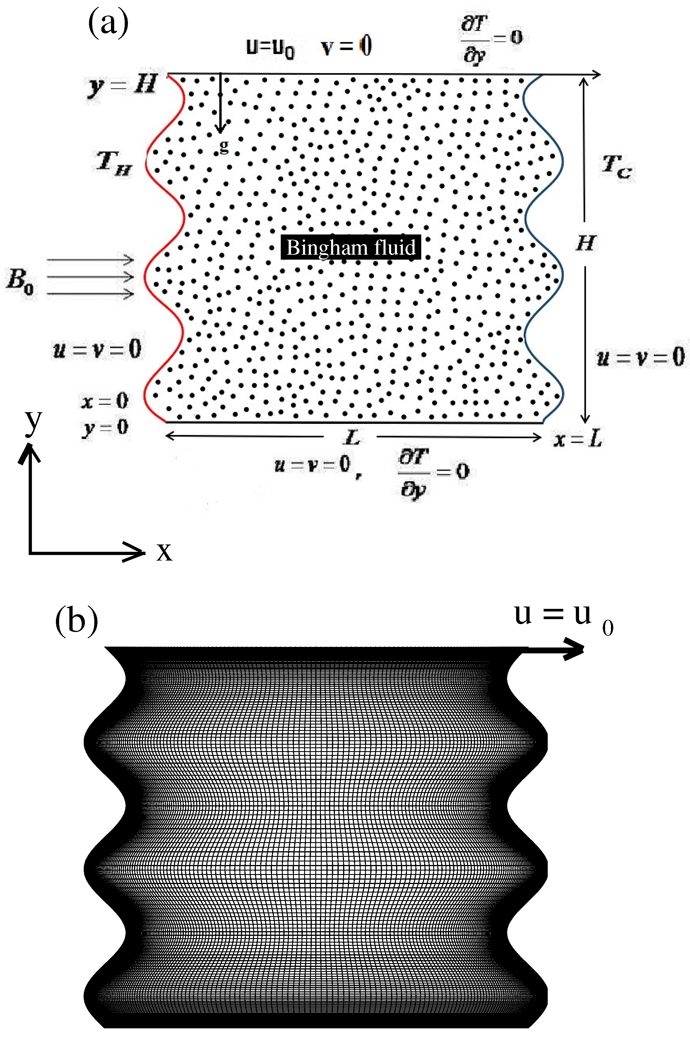
2.1. Physical Model Description
2.2. Bingham Model
2.3. Physical Properties of Non-Newtonian Bingham Nanofluid
2.4. Governing Dimensional Equations
2.5. Non-Dimensional Governing Equations
2.6. Rate of Heat Transfer
2.7. Entropy Generation
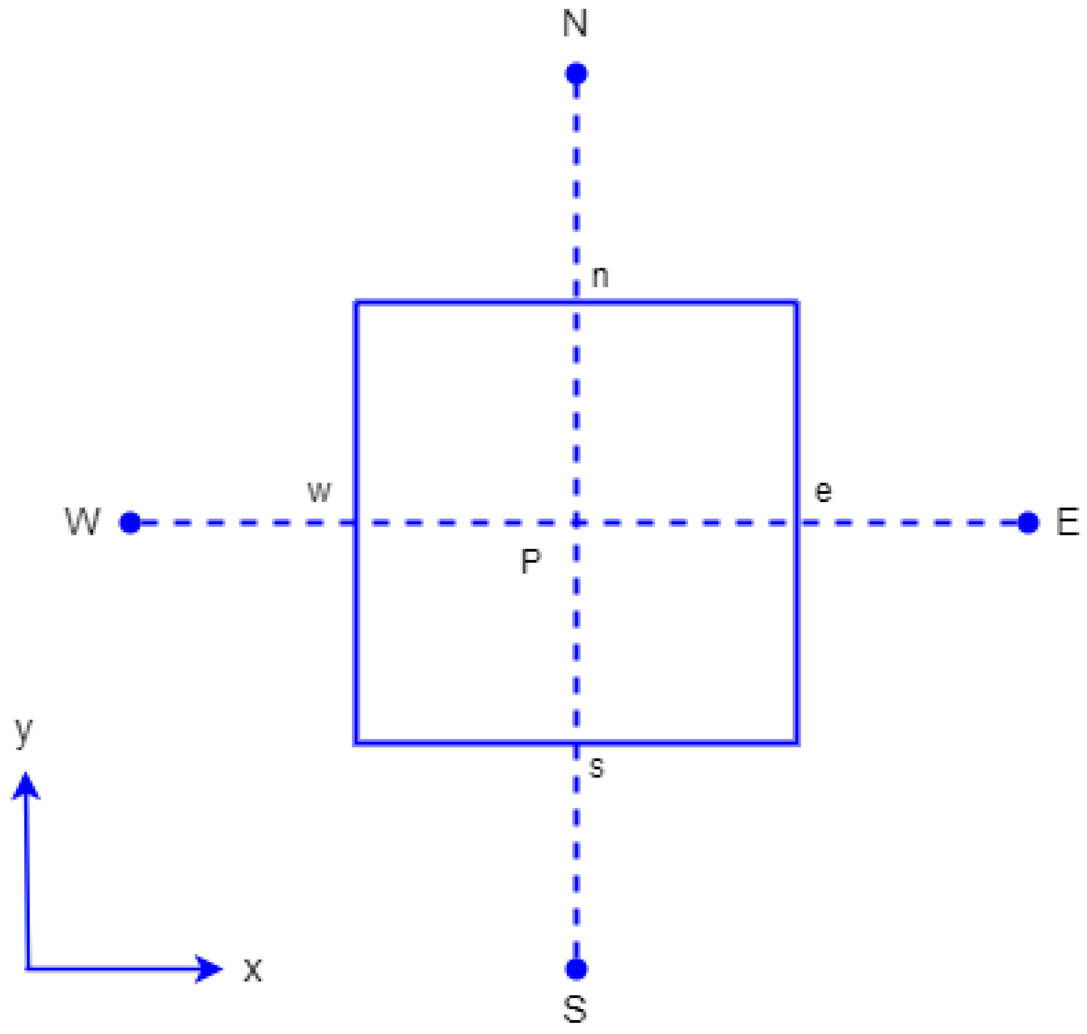
3. Numerical Methodology
4. Grid Independence Test and Code Validation
4.1. Grid Independence Test
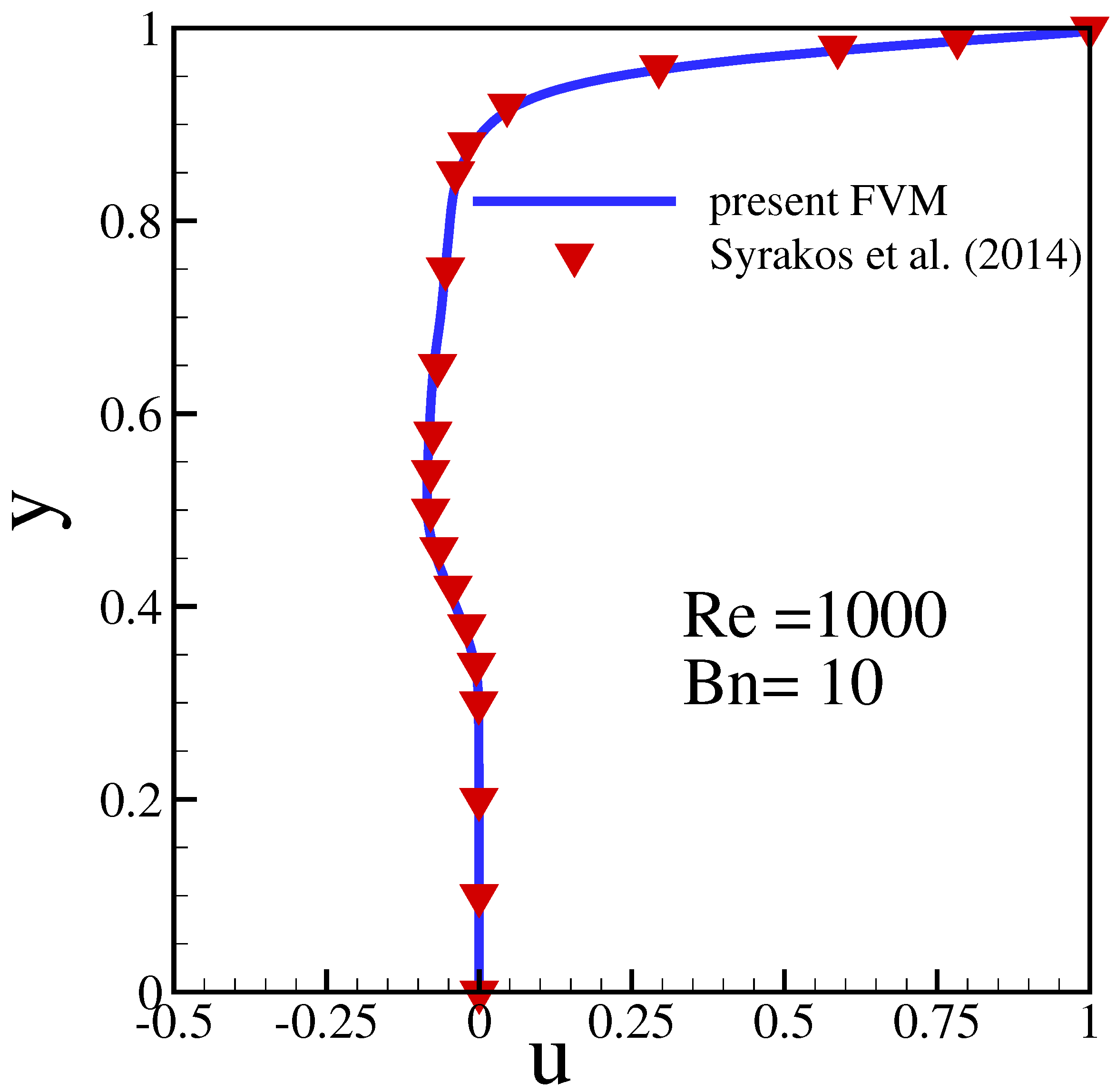
4.2. Code Validation for the Bingham Fluids
5. Results and Discussion
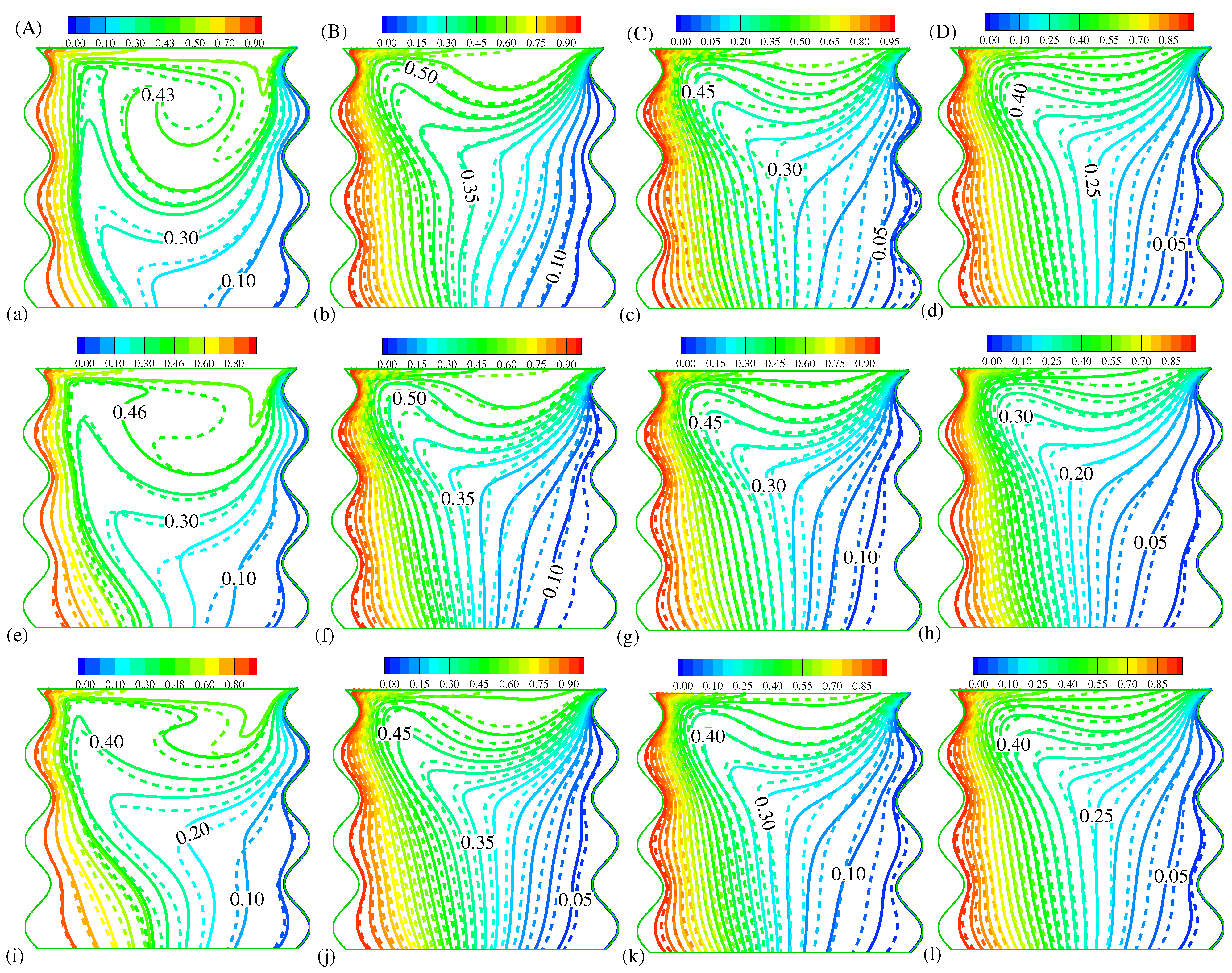
5.1. Temperature Distributions for various , , and
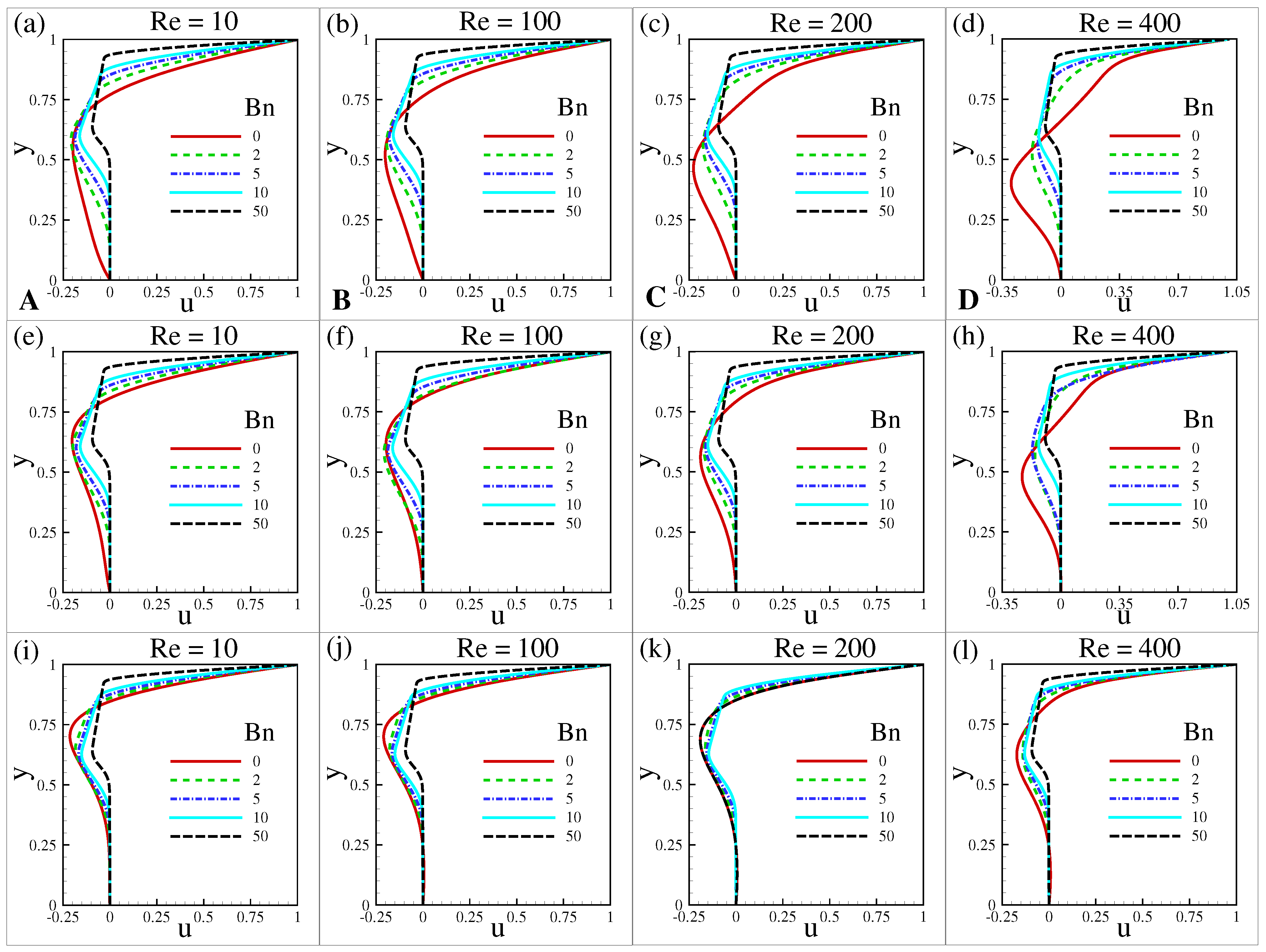
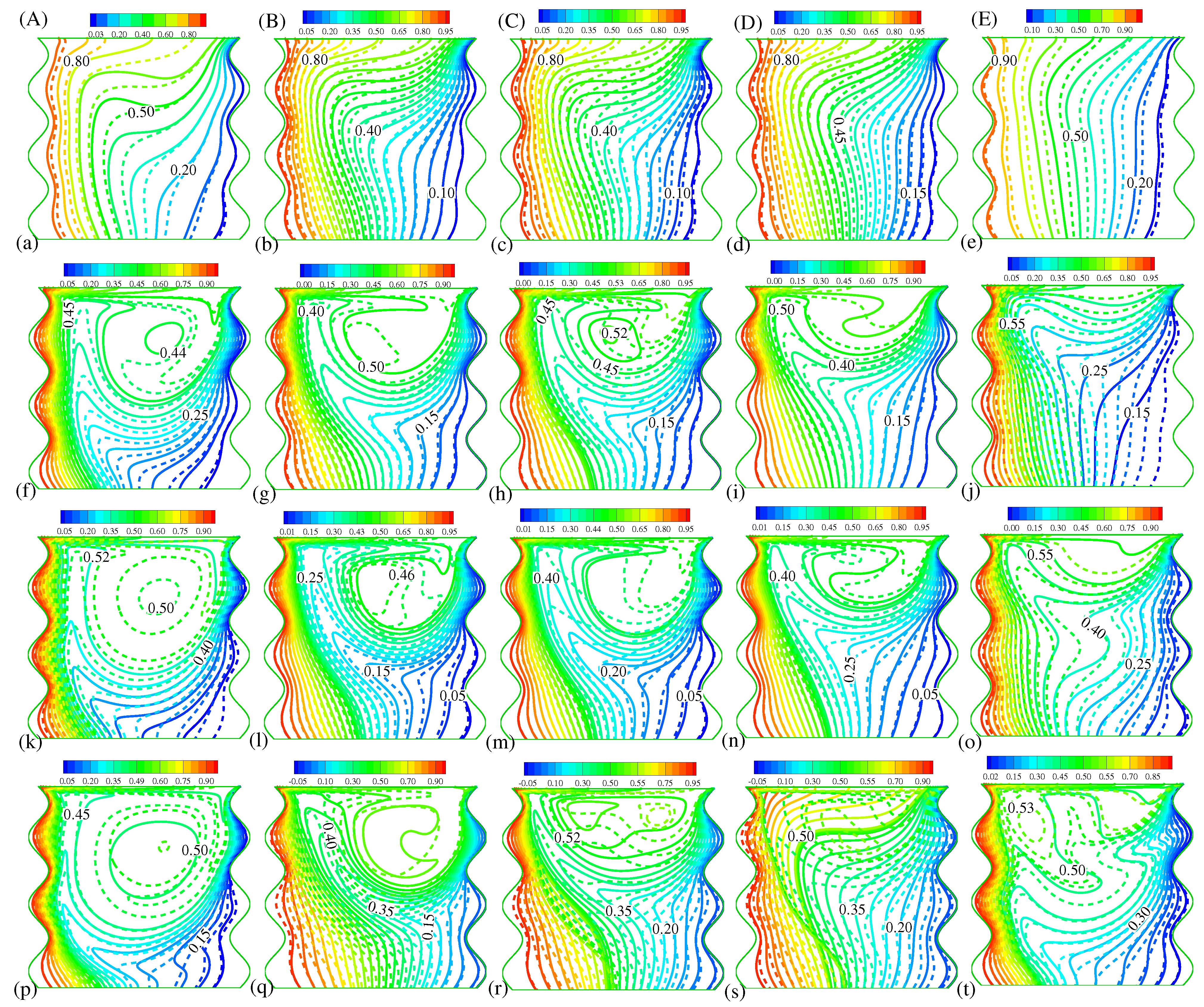
5.2. Effects of , , and on Streamlines at a Fixed
5.3. Effects of , , and on Streamlines at a Fixed
5.4. Effects of , , and on Isotherms at a Fixed
5.5. Effects of , , and on Isotherms at a Fixed
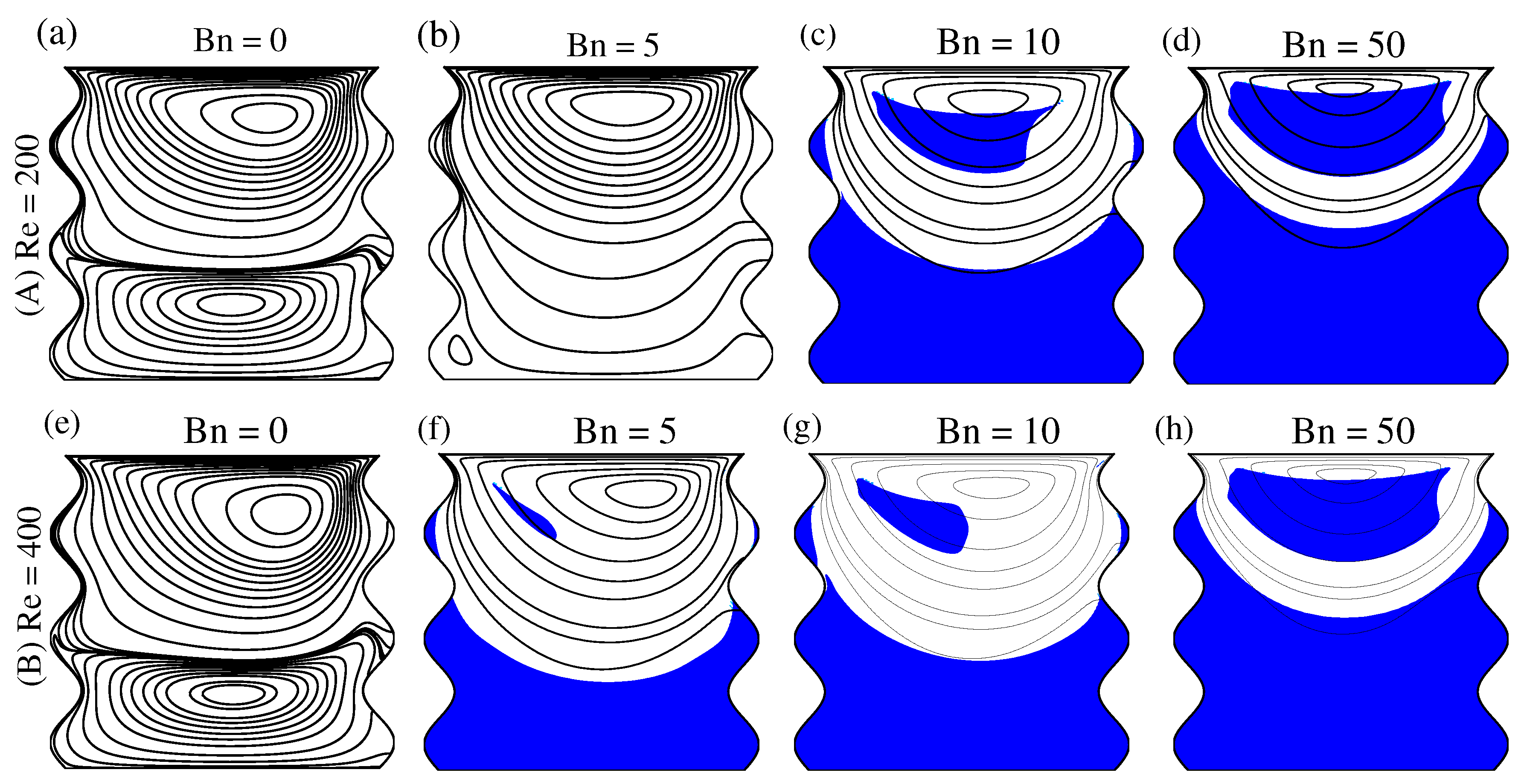
5.6. Effects of and on Unyielded Zone
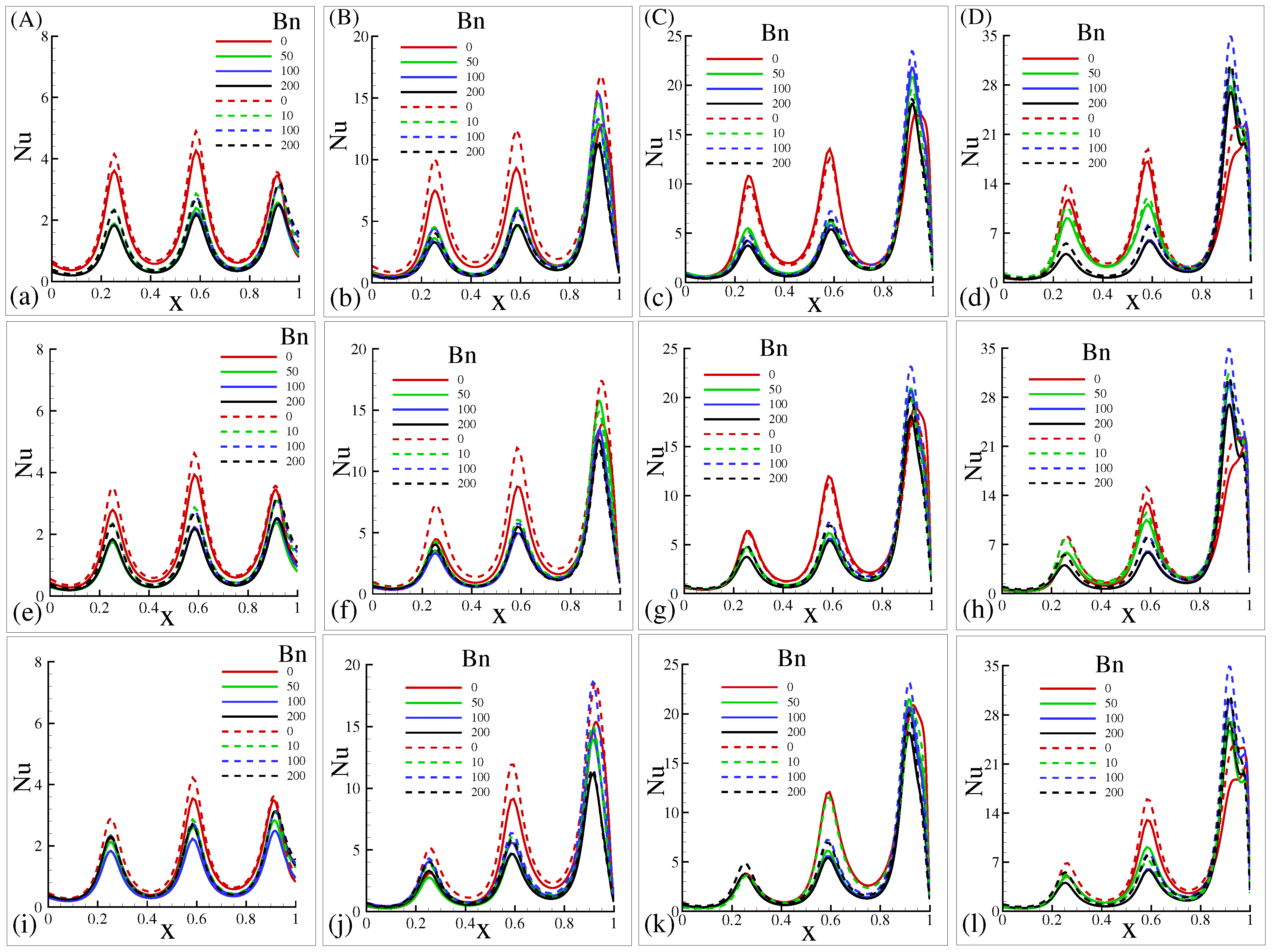
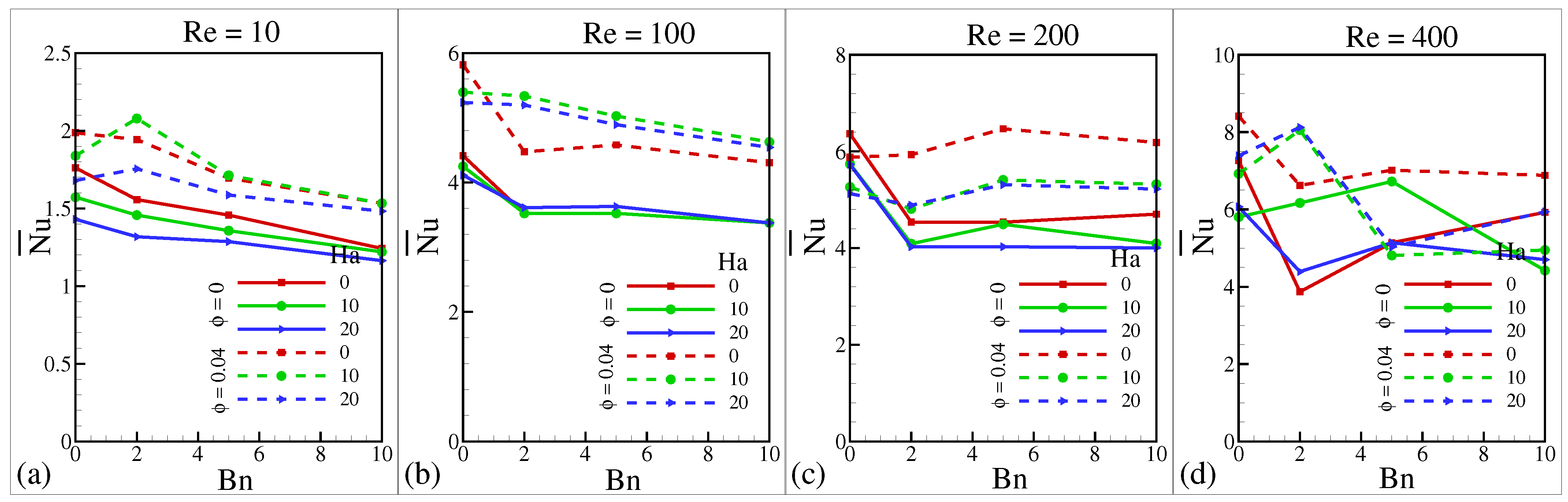
5.7. Effect of and on Local Nusselt Number ()
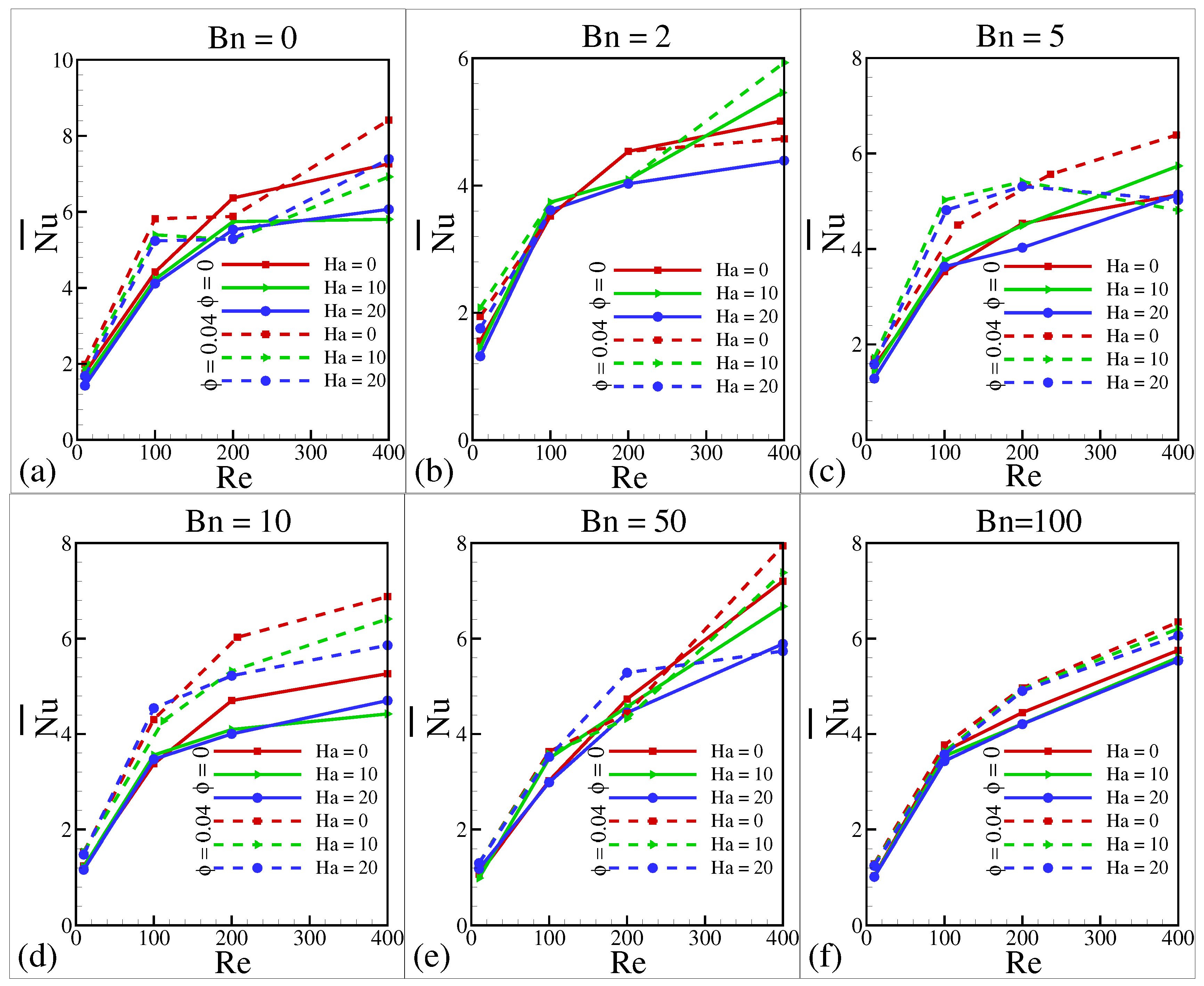
5.8. Effect of , , , and on Average Nusselt Number ()
5.9. Entropy Production for Various , , and
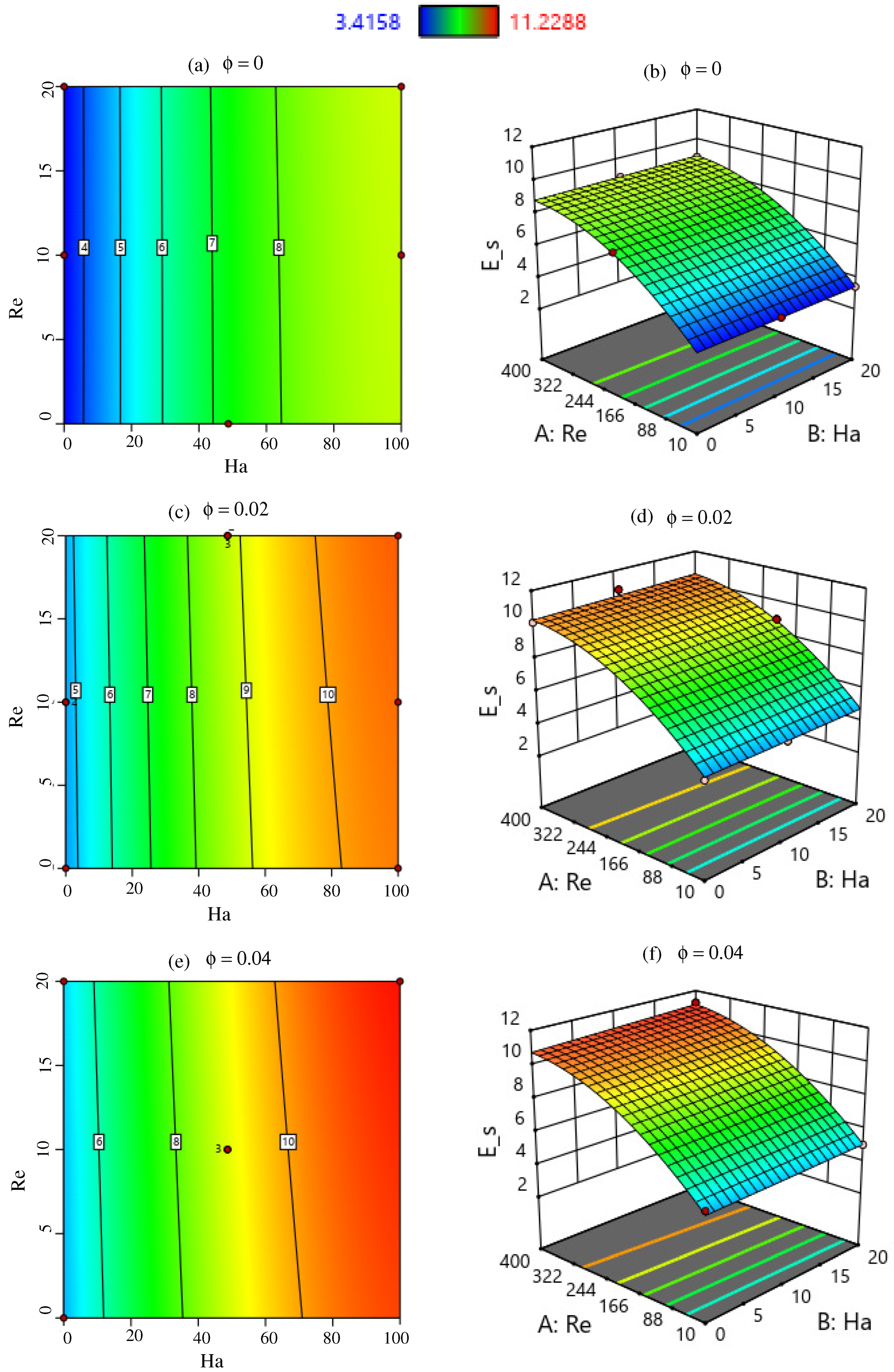
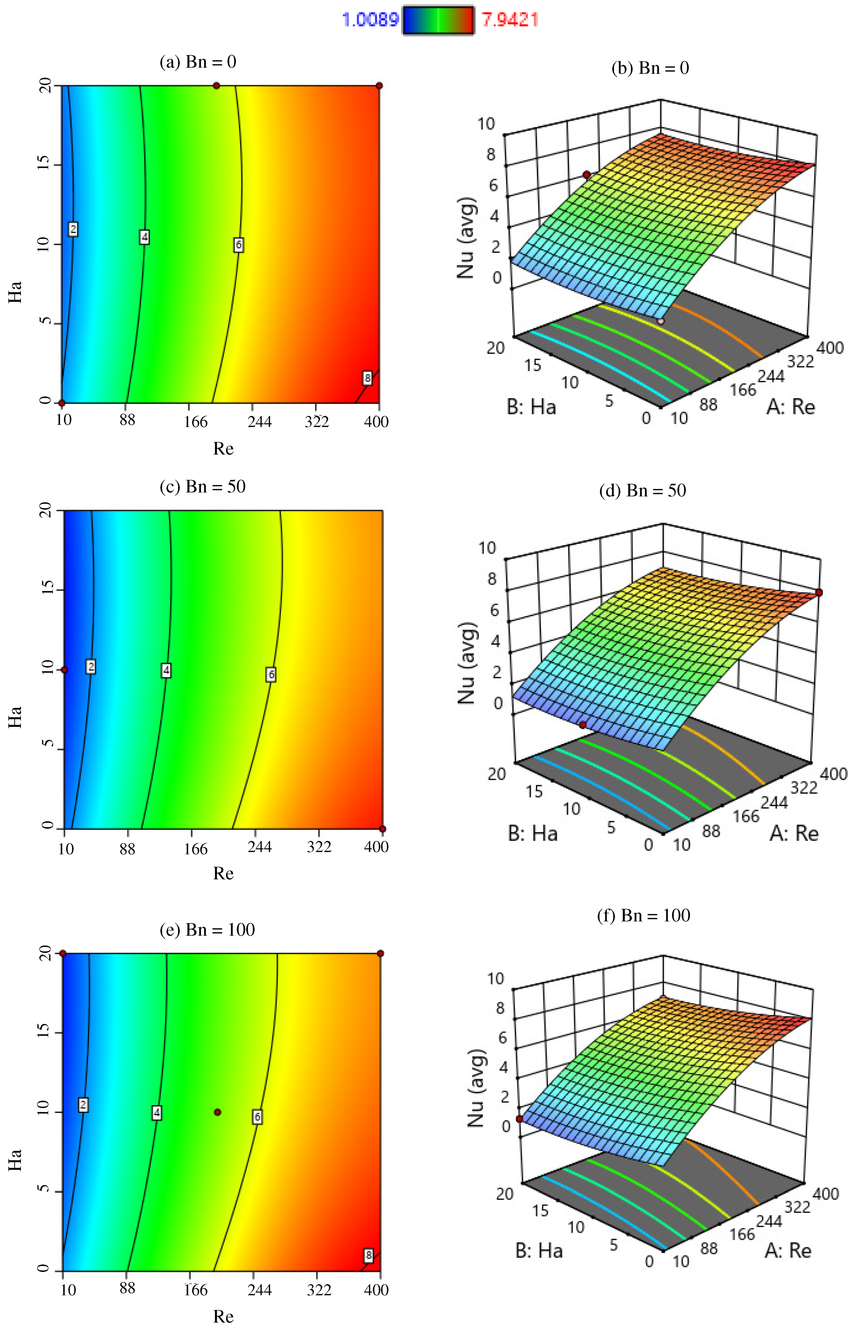
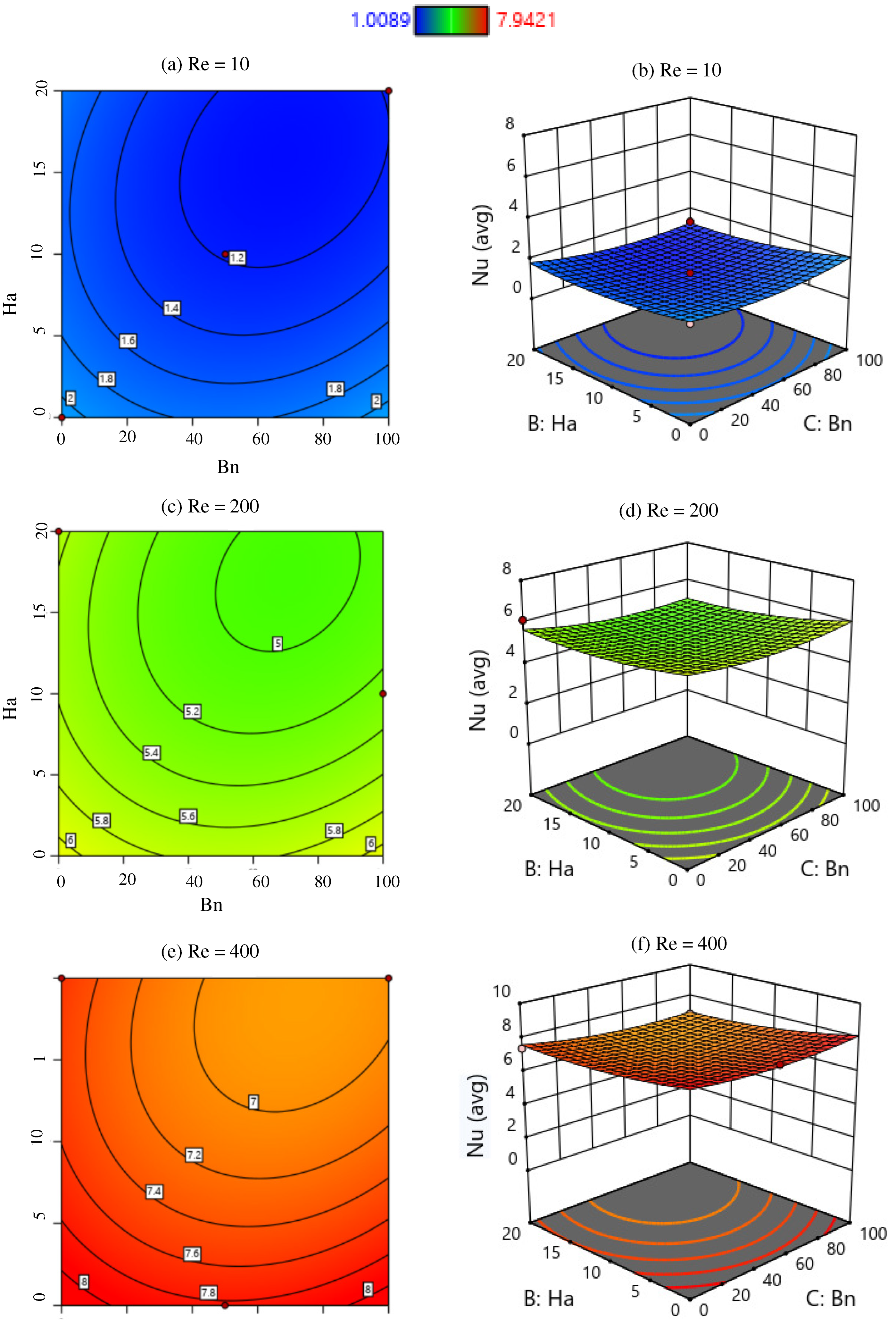
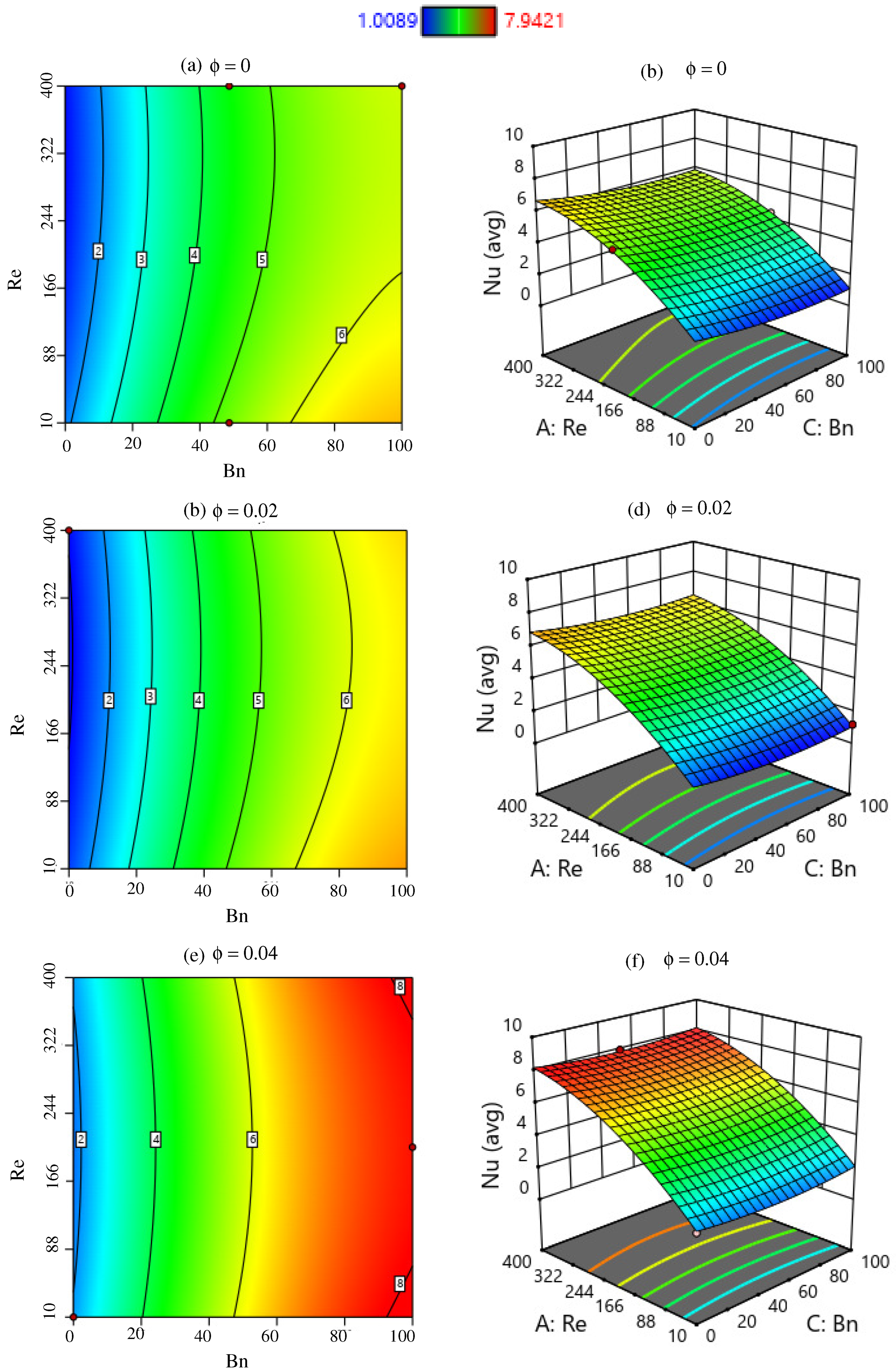
6. Response Surface Methodology of
Model Contour and Response Surface Plot
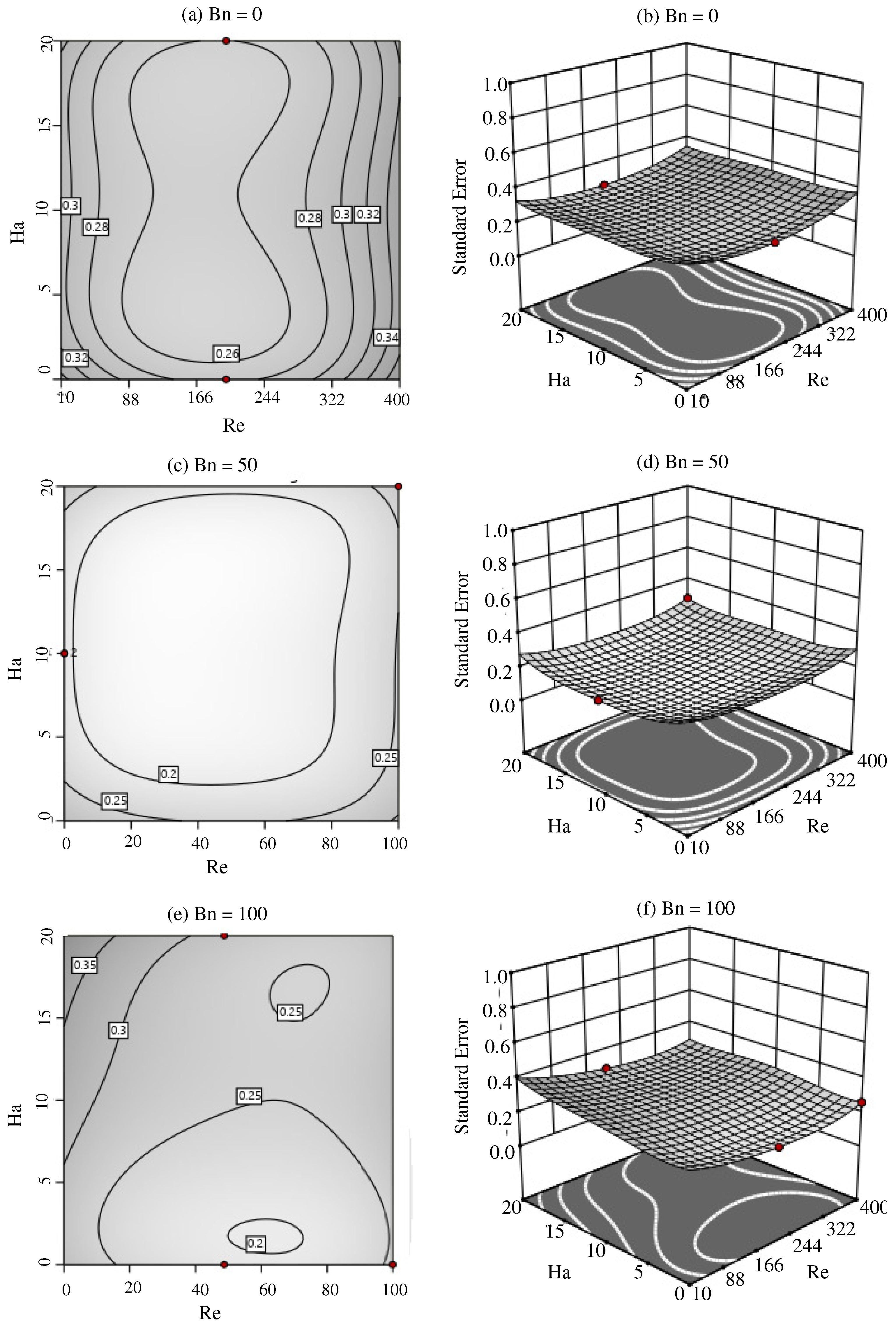
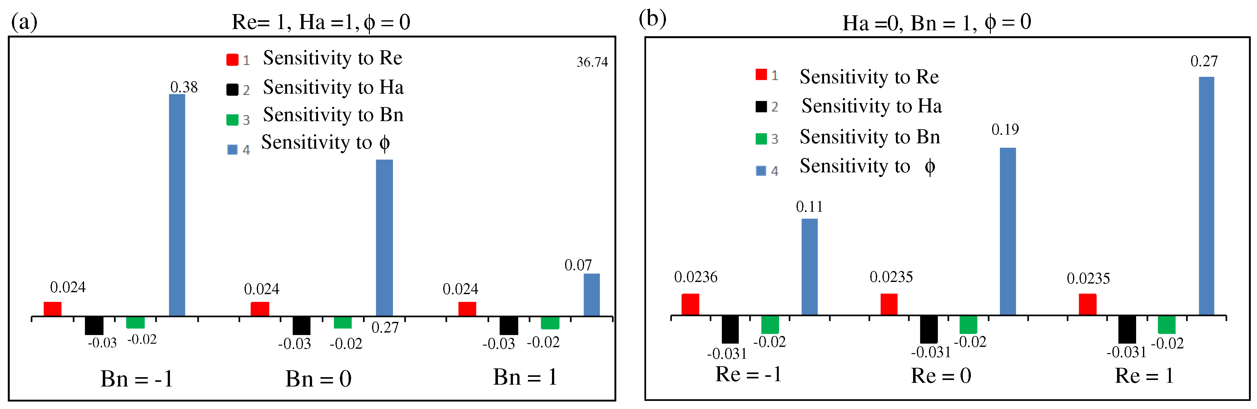
7. Sensitivity Analysis
8. Conclusions
- For non-Newtonian Bingham fluids, the Hartmann number (), Reynolds number (), Bingham number (), and nanoparticle volume fraction () all play an important role in the thermal velocity and temperature as well as the local and average rate of heat transfer in the wavy cavity.
- Convective heat transmission in a wavy cavity increases as and increase and decreases as and increase.
- The local rate of heat transfer increases as and increase. The highest magnitude of local is found at . This means that the local heat transfer rate is significant for the lower Richardson number (High ).
- High (low ) causes greater axial velocity within the wavy cavity. However, the addition of addition decreases u-velocity.
- The addition of an extra and nanoparticle volume fraction increases the magnitude of .
- At the highest and zero magnetic effect, the highest magnitude of has been found when extra nanoparticles are added to the simulation.
- , and have a significant impact on stream function, when and are progressively raised, tends to rise as well. However, is inversely proportional to and .
- As grows, the overall entropy production rises dramatically. When grows from 10 to 100, 100 to 200, and from 200 to 400 at and , increases by , , and respectively.
- The total entropy production is reduced when is increased. decreases by , , and , respectively, as grows from 0 to 20.
- At , the entropy production caused by the magnetic field is found to be 0. However, increases when an extra and of nanofluid are added to the system.
- The local Bejan number() does not show any significant changes in its magnitude. It shows a little variation with the change of different parameters (, , and ).
- The magnetic or Lorentz force reduces convective heat transport; as a result, , , , and velocity are reduced as increases.
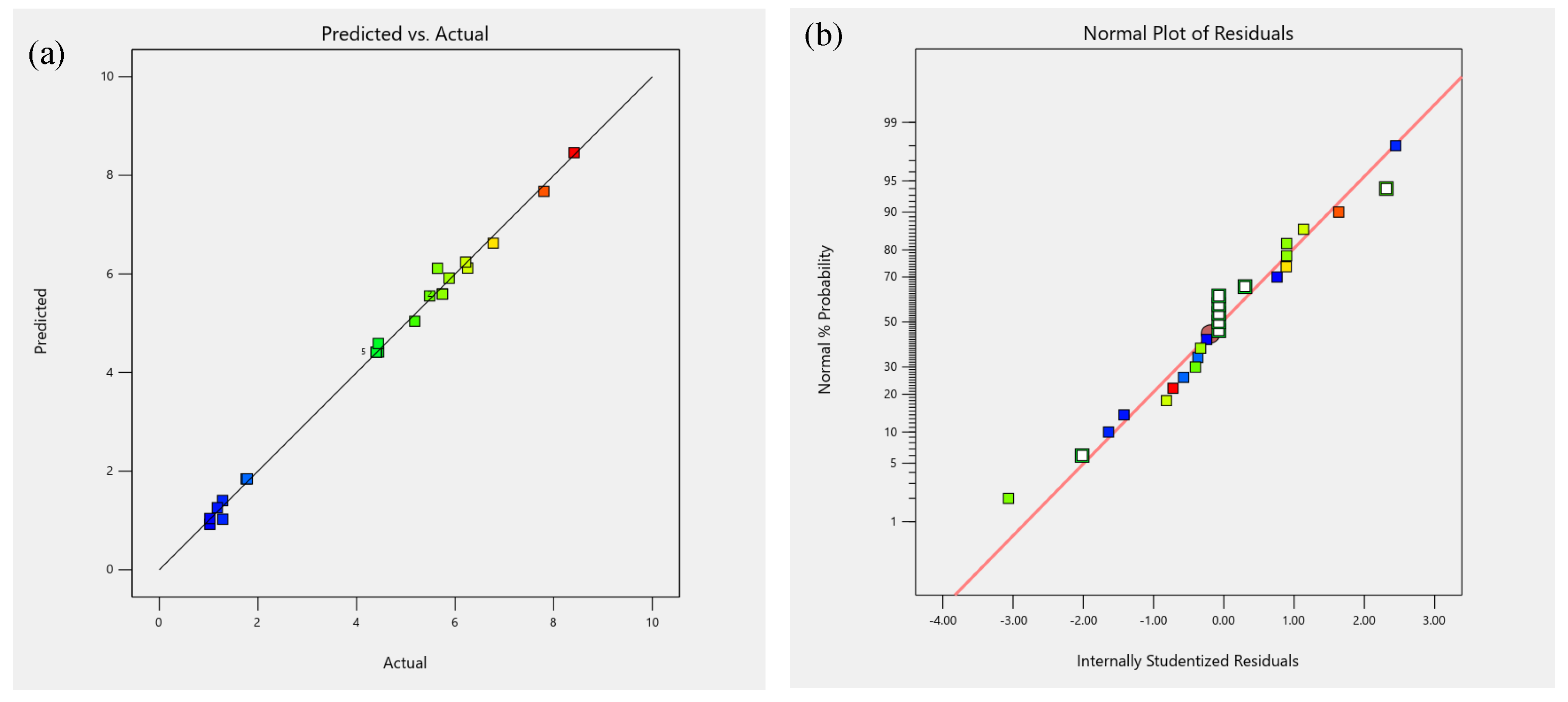
- The obtained correlation equation from the RSM method shows the relation of output responses to the input parameters.
- The and numbers have a positive sensitivity to the while the sensitivity of the and numbers is negative.
- The standard error of the RSM method is less negligible, and the obtained result from the RSM method shows an excellent agreement with the original CFD result.
Author Contributions
Funding
Data Availability Statement
Acknowledgments
Conflicts of Interest
Nomenclature
| English Symbols | ||
| Bingham number | ||
| Bejan number (Local) | ||
| Magnetic force | kg s A | |
| Specific heat | Jkg K | |
| E | Entropy production | J m s K |
| Grashof number | ||
| g | Gravitational acceleration | ms |
| Hartmann number | ||
| k | Thermal conductivity | J m s K |
| Nusselt number (Local) | ||
| Nusselt number (Average) | ||
| Prandtl number | ||
| Reynolds number | ||
| Richardson number | ||
| T | Temperature | K |
| Bulk temperature | K | |
| , | Dimensional mid-x and mid-y velocity components | ms |
| Dimensionless mid-x and mid-y velocity components | ||
| Dimensional coordinates | m | |
| Dimensionless coordinates | ||
| Greek Letters | ||
| Thermal diffusivity | ms | |
| Thermal expansion coefficient | K | |
| Dynamic viscosity | kg ms | |
| Kinematic viscosity | m s | |
| Fluid density | kg m | |
| Electrical conductivity | Am | |
| Volume fraction | ||
| Dimensionless stream function |
References
- Basak, T.; Roy, S.; Sharma, P.K.; Pop, I. Analysis of mixed convection flows within a square cavity with uniform and non-uniform heating of bottom wall. Int. J. Therm. Sci. 2009, 48, 891–912. [Google Scholar] [CrossRef]
- Waheed, M. Mixed convective heat transfer in rectangular enclosures driven by a continuously moving horizontal plate. Int. J. Heat Mass Transf. 2009, 52, 5055–5063. [Google Scholar] [CrossRef]
- Deswita, L.; Nazar, R.; Ishak, A.; Ahmad, R.; Pop, I. Similarity solutions for mixed convection boundary layer flow over a permeable horizontal flat plate. Appl. Math. Comput. 2010, 217, 2619–2630. [Google Scholar] [CrossRef]
- Iwatsu, R.; Hyun, J.M.; Kuwahara, K. Mixed convection in a driven cavity with a stable vertical temperature gradient. Int. J. Heat Mass Transf. 1993, 36, 1601–1608. [Google Scholar] [CrossRef]
- Sheremet, M.A.; Pop, I. Mixed convection in a lid-driven square cavity filled by a nanofluid: Buongiorno’s mathematical model. Appl. Math. Comput. 2015, 266, 792–808. [Google Scholar] [CrossRef]
- Stanisław, M.; Sylwia, D. A Class of Variational–Hemivariational Inequalities for Bingham Type Fluids. Appl. Math. Optim. 2022, 85, 16. [Google Scholar]
- Chhabra, R.P.; Richardson, J.F. Non-Newtonian Flow in the Process Industries: Fundamentals and Engineering Applications; Butterworth-Heinemann: Oxford, UK, 1999. [Google Scholar]
- Gupta, A.K.; Chhabra, R. Mixed convection from a spheroid in Bingham plastic fluids: Effect of buoyancy-assisted flow. Numer. Heat Transf. Part A Appl. 2016, 69, 898–920. [Google Scholar] [CrossRef]
- Vasco, D.A.; Moraga, N.O.; Haase, G. Parallel finite volume method simulation of three-dimensional fluid flow and convective heat transfer for viscoplastic non-Newtonian fluids. Numer. Heat Transf. Part A Appl. 2014, 66, 990–1019. [Google Scholar] [CrossRef]
- Saramito, P. A new elastoviscoplastic model based on the Herschel–Bulkley viscoplastic model. J. Non-Newton. Fluid Mech. 2009, 158, 154–161. [Google Scholar] [CrossRef]
- Huilgol, R.R.; You, Z. Application of the augmented Lagrangian method to steady pipe flows of Bingham, Casson and Herschel–Bulkley fluids. J. Non-Newton. Fluid Mech. 2005, 128, 126–143. [Google Scholar] [CrossRef]
- Papanastasiou, T.C. Flows of materials with yield. J. Rheol. 1987, 31, 385–404. [Google Scholar] [CrossRef]
- Mehmood, K.; Hussain, S.; Sagheer, M. Mixed convection in alumina-water nanofluid filled lid-driven square cavity with an isothermally heated square blockage inside with magnetic field effect: Introduction. Int. J. Heat Mass Transf. 2017, 109, 397–409. [Google Scholar] [CrossRef]
- Kumar, M.D.; Raju, C.; Sajjan, K.; El-Zahar, E.R.; Shah, N.A. Linear and quadratic convection on 3D flow with transpiration and hybrid nanoparticles. Int. Commun. Heat Mass Transf. 2022, 134, 105995. [Google Scholar] [CrossRef]
- Khaliq, S.; Abbas, Z. A theoretical analysis of roll-over-web coating assessment of viscous nanofluid containing Cu-water nanoparticles. J. Plast. Film. Sheeting 2020, 36, 55–75. [Google Scholar] [CrossRef]
- Siddiqa, S.; Molla, M.M.; Naqvi, S.B. Carreau ferrofluid flow with inclined magnetic field in an enclosure having heated cylinder. Phys. Scr. 2021, 96, 105007. [Google Scholar] [CrossRef]
- Ashraf, M.Z.; Rehman, S.U.; Farid, S.; Hussein, A.K.; Ali, B.; Shah, N.A.; Weera, W. Insight into significance of bioconvection on MHD tangent hyperbolic nanofluid flow of irregular thickness across a slender elastic surface. Mathematics 2022, 10, 2592. [Google Scholar] [CrossRef]
- Rashidi, S.; Mahian, O.; Languri, E.M. Applications of nanofluids in condensing and evaporating systems. J. Therm. Anal. Calorim. 2018, 131, 2027–2039. [Google Scholar] [CrossRef]
- Yang, L.; Ji, W.; Huang, J.n.; Xu, G. An updated review on the influential parameters on thermal conductivity of nano-fluids. J. Mol. Liq. 2019, 296, 111780. [Google Scholar] [CrossRef]
- Heris, S.Z.; Esfahany, M.N.; Etemad, G. Numerical investigation of nanofluid laminar convective heat transfer through a circular tube. Numer. Heat Transf. Part A Appl. 2007, 52, 1043–1058. [Google Scholar] [CrossRef]
- Lajvardi, M.; Moghimi-Rad, J.; Hadi, I.; Gavili, A.; Isfahani, T.D.; Zabihi, F.; Sabbaghzadeh, J. Experimental investigation for enhanced ferrofluid heat transfer under magnetic field effect. J. Magn. Magn. Mater. 2010, 322, 3508–3513. [Google Scholar] [CrossRef]
- Hojjat, M.; Etemad, S.G.; Bagheri, R.; Thibault, J. Rheological characteristics of non-Newtonian nanofluids: Experimental investigation. Int. Commun. Heat Mass Transf. 2011, 38, 144–148. [Google Scholar] [CrossRef]
- Nadooshan, A.A.; Eshgarf, H.; Afrand, M. Measuring the viscosity of Fe3O4-MWCNTs/EG hybrid nanofluid for evaluation of thermal efficiency: Newtonian and non-Newtonian behavior. J. Mol. Liq. 2018, 253, 169–177. [Google Scholar] [CrossRef]
- Barnoon, P.; Toghraie, D.; Dehkordi, R.B.; Afrand, M. Two phase natural convection and thermal radiation of Non-Newtonian nanofluid in a porous cavity considering inclined cavity and size of inside cylinders. Int. Commun. Heat Mass Transf. 2019, 108, 104285. [Google Scholar] [CrossRef]
- Tiwari, A.K.; Chhabra, R. Mixed convection in power-law fluids from a heated semicircular cylinder: Effect of aiding buoyancy. Numer. Heat Transf. Part A Appl. 2015, 67, 330–356. [Google Scholar] [CrossRef]
- Kuhlmann, H.; Wanschura, M.; Rath, H. Flow in two-sided lid-driven cavities: Non-uniqueness, instabilities, and cellular structures. J. Fluid Mech. 1997, 336, 267–299. [Google Scholar] [CrossRef]
- Mitsoulis, E. Flows of viscoplastic materials: Models and computations Rheol. Comp. Struct. 2007, 64, 677–694. [Google Scholar]
- Bercovier, M.; Engelman, M. A finite-element method for incompressible non-Newtonian flows. J. Comput. Phys. 1980, 36, 313–326. [Google Scholar] [CrossRef]
- Mitsoulis, E. On creeping drag flow of a viscoplastic fluid past a circular cylinder: Wall effects. Chem. Eng. Sci. 2004, 59, 789–800. [Google Scholar] [CrossRef]
- Mitsoulis, E.; Marangoudakis, S.; Spyratos, M.; Zisis, T.; Malamataris, N.A. Pressure-driven flows of Bingham plastics over a square cavity. J. Fluids Eng. Sep. 2006, 128, 993–1003. [Google Scholar] [CrossRef]
- Mitsoulis, E.; Zisis, T. Flow of Bingham plastics in a lid-driven square cavity. J. Non-Newton. Fluid Mech. 2001, 101, 173–180. [Google Scholar] [CrossRef]
- Vola, D.; Boscardin, L.; Latché, J. Laminar unsteady flows of Bingham fluids: A numerical strategy and some benchmark results. J. Comput. Phys. 2003, 187, 441–456. [Google Scholar] [CrossRef]
- Neofytou, P. A 3rd order upwind finite volume method for generalised Newtonian fluid flows. Adv. Eng. Softw. 2005, 36, 664–680. [Google Scholar] [CrossRef]
- Syrakos, A.; Georgiou, G.C.; Alexandrou, A.N. Solution of the square lid-driven cavity flow of a Bingham plastic using the finite volume method. J. Non-Newton. Fluid Mech. 2013, 195, 19–31. [Google Scholar] [CrossRef]
- Syrakos, A.; Georgiou, G.C.; Alexandrou, A.N. Performance of the finite volume method in solving regularised Bingham flows: Inertia effects in the lid-driven cavity flow. J. Non-Newton. Fluid Mech. 2014, 208, 88–107. [Google Scholar] [CrossRef]
- Rafiee, A. Modelling of generalized Newtonian lid-driven cavity flow using an SPH method. ANZIAM J. 2008, 49, 411–422. [Google Scholar] [CrossRef]
- dos Santos, D.D.; Frey, S.; Naccache, M.F.; de Souza Mendes, P. Numerical approximations for flow of viscoplastic fluids in a lid-driven cavity. J. Non-Newton. Fluid Mech. 2011, 166, 667–679. [Google Scholar] [CrossRef]
- Mahmood, R.; Kousar, N.; Yaqub, M.; Jabeen, K. Numerical simulations of the square lid driven cavity flow of Bingham fluids using nonconforming finite elements coupled with a direct solver. Adv. Math. Phys. 2017, 2017, 5210708. [Google Scholar] [CrossRef]
- Ghanbarpour, M.; Haghigi, E.B.; Khodabandeh, R. Thermal properties and rheological behavior of water based Al2O3 nanofluid as a heat transfer fluid. Exp. Therm. Fluid Sci. 2014, 53, 227–235. [Google Scholar] [CrossRef]
- Huilgol, R.R. Fluid Mechanics of Viscoplasticity; Springer: Berlin/Heidelberg, Germany, 2015. [Google Scholar]
- Sanchez, F. Application of a first-order operator splitting method to Bingham fluid flow simulation. Comput. Math. Appl. 1998, 36, 71–86. [Google Scholar] [CrossRef]
- Dean, E.; Glowinski, R. Operator-splitting methods for the simulation of Bingham visco-plastic flow. Chin. Ann. Math. 2002, 23, 187–204. [Google Scholar] [CrossRef]
- Huilgol, R.; Kefayati, G. Natural convection problem in a Bingham fluid using the operator-splitting method. J. Non-Newton. Fluid Mech. 2015, 220, 22–32. [Google Scholar] [CrossRef]
- Chhabra, R.P.; Richardson, J.F. Non-Newtonian Flow and Applied Rheology: Engineering Applications; Butterworth-Heinemann: Oxford, UK, 2011. [Google Scholar]
- Chhabra, R. Fluid mechanics and heat transfer with non-Newtonian liquids in mechanically agitated vessels. Adv. Heat Transf. 2003, 37, 77–178. [Google Scholar]
- Paul, E.L.; Atiemo-Obeng, V.A.; Kresta, S.M. Handbook of Industrial Mixing: Science and Practice; John Wiley & Sons: Hoboken, NJ, USA, 2003; Volume 1. [Google Scholar]
- Chhabra, R.P. Bubbles, Drops, and Particles in Non-Newtonian Fluids; CRC Press: Boca Raton, FL, USA, 2006. [Google Scholar]
- Chhabra, R.P.; Comiti, J.; Machač, I. Flow of non-Newtonian fluids in fixed and fluidised beds. Chem. Eng. Sci. 2001, 56, 1–27. [Google Scholar] [CrossRef]
- Nirmalkar, N.; Chhabra, R.; Poole, R. Effect of shear-thinning behavior on heat transfer from a heated sphere in yield-stress fluids. Ind. Eng. Chem. Res. 2013, 52, 13490–13504. [Google Scholar] [CrossRef]
- Gumulya, M.; Horsley, R.; Pareek, V. Numerical simulation of the settling behaviour of particles in thixotropic fluids. Phys. Fluids 2014, 26, 023102. [Google Scholar] [CrossRef]
- Nirmalkar, N.; Chhabra, R.; Poole, R. On creeping flow of a Bingham plastic fluid past a square cylinder. J. Non-Newton. Fluid Mech. 2012, 171, 17–30. [Google Scholar] [CrossRef]
- Zisis, T.; Mitsoulis, E. Viscoplastic flow around a cylinder kept between parallel plates. J. Non-Newton. Fluid Mech. 2002, 105, 1–20. [Google Scholar] [CrossRef]
- Duvant, G.; Lions, J.L. Inequalities in Mechanics and Physics; Springer Science & Business Media: Berlin/Heidelberg, Germany, 2012; Volume 219. [Google Scholar]
- Baranovskii, E.S. On flows of Bingham-type fluids with threshold slippage. Adv. Math. Phys. 2017, 2017, 7548328. [Google Scholar] [CrossRef]
- Thohura, S.; Molla, M.M.; Sarker, M. Bingham fluid flow simulation in a lid-driven skewed cavity using the finite-volume method. Int. J. Comput. Math. 2020, 97, 1212–1233. [Google Scholar] [CrossRef]
- Xuan, Y.; Li, Q. Heat transfer enhancement of nanofluids. Int. J. Heat Fluid Flow 2000, 21, 58–64. [Google Scholar] [CrossRef]
- Hossain, A.; Nag, P.; Molla, M.M. Mesoscopic Simulation of MHD Mixed Convection of Non-Newtonian Ferrofluids with a Non-uniformly Heated Plate in an Enclosure. Phys. Scr. 2022, 98, 015008. [Google Scholar] [CrossRef]
- Javed, T.; Siddiqui, M.A. Effect of MHD on heat transfer through ferrofluid inside a square cavity containing obstacle/heat source. Int. J. Therm. Sci. 2018, 125, 419–427. [Google Scholar] [CrossRef]
- Sheremet, M.A.; Oztop, H.; Pop, I.; Al-Salem, K. MHD free convection in a wavy open porous tall cavity filled with nanofluids under an effect of corner heater. Int. J. Heat Mass Transf. 2016, 103, 955–964. [Google Scholar] [CrossRef]
- Corcione, M.; Cianfrini, M.; Quintino, A. Two-phase mixture modeling of natural convection of nanofluids with temperature-dependent properties. Int. J. Therm. Sci. 2013, 71, 182–195. [Google Scholar] [CrossRef]
- Cianfrini, M.; Corcione, M.; Quintino, A. Natural convection in square enclosures differentially heated at sides using alumina-water nanofluids with temperature-dependent physical properties. Therm. Sci. 2015, 19, 591–608. [Google Scholar] [CrossRef]
- Kefayati, G.R. Mesoscopic simulation of mixed convection on non-Newtonian nanofluids in a two sided lid-driven enclosure. Adv. Powder Technol. 2015, 26, 576–588. [Google Scholar] [CrossRef]
- Kefayati, G.R. Mixed convection of non-Newtonian nanofluids flows in a lid-driven enclosure with sinusoidal temperature profile using FDLBM. Powder Technol. 2014, 266, 268–281. [Google Scholar] [CrossRef]
- Abu-Nada, E.; Chamkha, A.J. Mixed convection flow in a lid-driven inclined square enclosure filled with a nanofluid. Eur. J. Mech.-B/Fluids 2010, 29, 472–482. [Google Scholar] [CrossRef]
- Afsana, S.; Molla, M.M.; Nag, P.; Saha, L.K.; Siddiqa, S. MHD natural convection and entropy generation of non-Newtonian ferrofluid in a wavy enclosure. Int. J. Mech. Sci. 2021, 198, 106350. [Google Scholar] [CrossRef]
- Islam, M.; Hai, S.A.; Nag, P.; Molla, M.M. Multiple-relaxation-time lattice Boltzmann simulation of free convection and irreversibility of nanofluid with variable thermophysical properties. Phys. Scr. 2021, 96, 125031. [Google Scholar] [CrossRef]
- Hatami, M. Cross-sectional heat transfer of hot tubes in a wavy porous channel filled by Fe3O4–water nanofluid under a variable magnetic field. Eur. Phys. J. Plus 2018, 133, 374. [Google Scholar] [CrossRef]
- Sheikholeslami, M.; Rashidi, M.M. Effect of space dependent magnetic field on free convection of Fe3O4–water nanofluid. J. Taiwan Inst. Chem. Eng. 2015, 56, 6–15. [Google Scholar] [CrossRef]
- Hasan, M.F.; Himika, T.A.; Molla, M.M. Lattice Boltzmann Method with Large-Eddy Simulation of Airflow and Mixed Convection in a General Ward of Hospital. J. Comput. Eng. 2016, 2016, 1–15. [Google Scholar]
- Kahalerras, H.; Fersadou, B.; Nessab, W. Mixed convection heat transfer and entropy generation analysis of copper–water nanofluid in a vertical channel with non-uniform heating. SN Appl. Sci. 2020, 2, 1–12. [Google Scholar] [CrossRef]
- Bejan, A. Entropy Generation Minimization: The Method of Thermodynamic Optimization of Finite-Size Systems and Finite-Time Processes; CRC Press: Boca Raton, FL, USA, 2013. [Google Scholar]
- Thohura, S.; Molla, M.M.; Sarker, M. Numerical simulation of Bingham fluid flows in a lid-driven skewed cavity. AIP Conf. Proc. 2018, 1980, 040022. [Google Scholar]
- Molla, M.M. LES of Pulsatile Flow in the Models of Arterial Stenosis and Aneurysm. Ph.D. Thesis, University of Glasgow, Glasgow, UK, 2009. [Google Scholar]
- Jones, W.P.; di Mare, F.; Marquis, A.J. LES-BOFFIN: User’s Guide; Imperial College: London, UK, 2002; pp. 1–60. [Google Scholar]
- Thohura, S.; Molla, M.M.; Sarker, M.M.A. Numerical simulation of non-Newtonian power-law fluid flow in a lid-driven skewed cavity. Int. J. Appl. Comput. Math. 2019, 5, 1–29. [Google Scholar] [CrossRef]
- Nirmalkar, N.; Bose, A.; Chhabra, R. Free convection from a heated circular cylinder in Bingham plastic fluids. Int. J. Therm. Sci. 2014, 83, 33–44. [Google Scholar] [CrossRef]
- Turan, O.; Sachdeva, A.; Chakraborty, N.; Poole, R.J. Laminar natural convection of power-law fluids in a square enclosure with differentially heated side walls subjected to constant temperatures. J. Non-Newton. Fluid Mech. 2011, 166, 1049–1063. [Google Scholar] [CrossRef]
- Aydm, O. Aiding and opposing mechanisms of mixed convection in a shear-and buoyancy-driven cavity. Int. Commun. Heat Mass Transf. 1999, 26, 1019–1028. [Google Scholar] [CrossRef]
- Awad, M.M. A new definition of Bejan number. Therm. Sci. 2012, 16, 1251–1253. [Google Scholar] [CrossRef]
- Awad, M. The science and the history of the two Bejan numbers. Int. J. Heat Mass Transf. 2016, 94, 101–103. [Google Scholar] [CrossRef]
- Myers, R.H.; Khuri, A.I.; Vining, G. Response surface alternatives to the Taguchi robust parameter design approach. Am. Stat. 1992, 46, 131–139. [Google Scholar]
- Hossain, A.; Anee, M.J.; Faruqui, R.; Bushra, S.; Rahman, P.; Khan, R. A GPS Based Unmanned Drone Technology for Detecting and Analyzing Air Pollutants. IEEE Instr. Meas. Mag. 2022, 25, 53–60. [Google Scholar] [CrossRef]
- Rashidi, S.; Bovand, M.; Esfahani, J.A. Optimization of partitioning inside a single slope solar still for performance improvement. Desalination 2016, 395, 79–91. [Google Scholar] [CrossRef]
- Rashidi, S.; Bovand, M.; Esfahani, J.A. Structural optimization of nanofluid flow around an equilateral triangular obstacle. Energy 2015, 88, 385–398. [Google Scholar] [CrossRef]
- Hossain, A.; Uddin, S.; Rahman, P.; Anee, M.J.; Rifat, M.M.H.; Uddin, M.M. Wavelet and Spectral Analysis of Normal and Abnormal Heart Sound for Diagnosing Cardiac Disorders. Bio. Res. Intl. 2022, 2022, 9092346. [Google Scholar] [CrossRef] [PubMed]
- Jawairia, S.; Raza, J. Optimization of heat transfer rate in a moving porous fin under radiation and natural convection by response surface methodology: Sensitivity analysis. Chem. Eng. J. Adv. 2022, 11, 100304. [Google Scholar] [CrossRef]
- Shirvan, K.M.; Mamourian, M.; Mirzakhanlari, S.; Ellahi, R.; Vafai, K. Numerical investigation and sensitivity analysis of effective parameters on combined heat transfer performance in a porous solar cavity receiver by response surface methodology. Int. J. Heat Mass Transf. 2017, 105, 811–825. [Google Scholar] [CrossRef]


| Average Nusselt Number | |||
|---|---|---|---|
| Grid size | |||
| G1: | 7.6854 (6.18%) | 7.0113 (2.48%) | 6.2924 (1.13%) |
| G2: | 7.2383 (0.00%) | 6.8416 (0.00%) | 6.2111 (0.00%) |
| G.3: | 7.1644 (1.02%) | 6.7711 (1.03%) | 6.1943 (0.27%) |
| 10 | 0 | 1.7606 | 1.5567 | 1.5567 | 1.2422 | 1.0709 | 1.0258 | 1.0196 | |
| 0 | 0.02 | 1.7843 | 2.0552 | 1.8890 | 1.8623 | 1.2370 | 1.1768 | 1.1488 | |
| 0.04 | 1.9869 | 1.9429 | 1.6947 | 1.5336 | 1.3028 | 1.2871 | 1.2855 | ||
| 0 | 1.5721 | 1.4566 | 1.4566 | 1.2201 | 1.0089 | 1.0255 | 1.0257 | ||
| 10 | 0.02 | 1.6502 | 1.9687 | 1.8272 | 1.5383 | 1.2008 | 1.1504 | 1.1180 | |
| 0.04 | 1.8387 | 2.0784 | 1.7125 | 1.5327 | 1.3050 | 1.2870 | 1.2849 | ||
| 0 | 1.4299 | 1.3173 | 1.2861 | 1.1635 | 1.1844 | 1.0248 | 1.2832 | ||
| 20 | 0.02 | 1.2833 | 2.3075 | 1.7655 | 1.4955 | 1.3901 | 1.5007 | 1.6011 | |
| 0.04 | 1.6795 | 1.7548 | 1.5861 | 1.4819 | 1.3029 | 1.2867 | 1.2767 | ||
| 100 | 0 | 4.4136 | 3.5236 | 3.5236 | 3.3759 | 3.6507 | 3.6388 | 2.7102 | |
| 0 | 0.02 | 5.2663 | 4.1961 | 4.2467 | 4.3277 | 3.3503 | 3.4276 | 3.5449 | |
| 0.04 | 5.8186 | 4.4742 | 4.5803 | 4.3060 | 3.6313 | 3.1696 | 3.0901 | ||
| 0 | 4.2487 | 3.7377 | 3.7642 | 3.5588 | 3.4906 | 3.0387 | 3.1499 | ||
| 10 | 0.02 | 5.0076 | 3.9359 | 4.3483 | 3.9546 | 3.3155 | 3.2293 | 3.0278 | |
| 0.04 | 5.1958 | 5.3358 | 5.0267 | 4.6271 | 3.5782 | 3.2294 | 2.9411 | ||
| 0 | 4.1120 | 3.6115 | 3.6301 | 3.4716 | 2.9876 | 3.4332 | 2.7071 | ||
| 20 | 0.02 | 5.0881 | 3.7390 | 4.1958 | 3.8338 | 3.5431 | 3.7101 | 3.0434 | |
| 0.04 | 5.2357 | 5.1968 | 4.8929 | 4.5422 | 4.7276 | 4.0709 | 3.0877 | ||
| 200 | 0 | 5.3654 | 4.5366 | 4.5366 | 4.7017 | 4.7345 | 4.4483 | 3.8059 | |
| 0 | 0.02 | 5.4823 | 4.9888 | 4.9888 | 5.2777 | 4.6943 | 4.8743 | 4.0159 | |
| 0.04 | 5.8789 | 5.9311 | 6.4690 | 6.1849 | 4.4321 | 4.9664 | 4.0709 | ||
| 0 | 5.7420 | 4.0906 | 4.4923 | 4.0954 | 4.5705 | 4.2128 | 3.8053 | ||
| 10 | 0.02 | 5.8672 | 5.2835 | 2.7265 | 3.1851 | 4.0908 | 4.4005 | 4.6398 | |
| 0.04 | 5.9247 | 4.8102 | 5.4107 | 5.3212 | 4.3242 | 4.9368 | 4.4449 | ||
| 0 | 5.7327 | 4.2277 | 4.0277 | 4.0030 | 4.4481 | 4.2078 | 3.8032 | ||
| 20 | 0.02 | 5.8821 | 3.9048 | 4.2257 | 3.0692 | 4.3857 | 4.7327 | 4.0060 | |
| 0.04 | 6.1255 | 4.8873 | 5.3112 | 5.2216 | 4.2855 | 4.9332 | 4.4433 | ||
| 400 | 0 | 7.2634 | 3.8699 | 5.1394 | 5.5567 | 7.2029 | 5.6446 | 5.1800 | |
| 0 | 0.02 | 7.8008 | 5.5638 | 6.4072 | 6.5531 | 7.8039 | 6.0052 | 6.1813 | |
| 0.04 | 8.4137 | 6.6223 | 7.0149 | 6.8813 | 7.9421 | 6.8459 | 6.2134 | ||
| 0 | 5.8036 | 6.1672 | 6.7236 | 4.4216 | 6.6753 | 5.6429 | 5.1795 | ||
| 10 | 0.02 | 6.3983 | 5.9977 | 5.9406 | 6.05091 | 6.9301 | 6.3452 | 6.6691 | |
| 0.04 | 6.9226 | 8.0508 | 4.8102 | 4.9496 | 7.3826 | 6.8449 | 6.2128 | ||
| 0 | 6.0679 | 4.3913 | 5.1394 | 4.7014 | 5.8887 | 5.6378 | 5.1779 | ||
| 20 | 0.02 | 7.0675 | 5.1829 | 6.3365 | 5.8752 | 6.1911 | 6.7734 | 6.2531 | |
| 0.04 | 7.3885 | 8.1243 | 5.0262 | 5.9388 | 7.2383 | 6.8416 | 6.2111 |
| 10 | 0 | 2.1775 | 1.2983 | 0 | 3.4748 | 0.9627 | |
| 0 | 0.02 | 3.0456 | 1.3893 | 0 | 4.4406 | 0.9523 | |
| 0.04 | 3.4097 | 1.6191 | 0 | 5.0288 | 0.9533 | ||
| 0 | 2.1766 | 1.2976 | 0.00049 | 3.4257 | 0.9629 | ||
| 10 | 0.02 | 3.0571 | 1.6002 | 0.00047 | 4.6602 | 0.9585 | |
| 0.04 | 3.4100 | 1.6187 | 0.00046 | 5.0292 | 0.9532 | ||
| 0 | 2.1755 | 1.2954 | 0.00192 | 3.4158 | 0.9629 | ||
| 20 | 0.02 | 3.1602 | 1.3400 | 0.00189 | 4.7410 | 1.0592 | |
| 0.04 | 3.4107 | 1.6176 | 0.00182 | 5.0301 | 0.9530 | ||
| 100 | 0 | 2.2023 | 3.8619 | 0 | 6.0643 | 0.9588 | |
| 0 | 0.02 | 3.2453 | 3.7403 | 0 | 6.9491 | 0.9894 | |
| 0.04 | 3.4470 | 3.7676 | 0 | 7.2146 | 0.9631 | ||
| 0 | 2.2026 | 3.4714 | 0.00049 | 5.6745 | 0.9666 | ||
| 10 | 0.02 | 3.2543 | 3.5047 | 0.00047 | 9.9501 | 0.9865 | |
| 0.04 | 3.4473 | 3.7967 | 0.00046 | 7.2444 | 0.9626 | ||
| 0 | 3.2033 | 3.7097 | 0.00191 | 5.9149 | 0.9615 | ||
| 20 | 0.02 | 4.0454 | 4.1949 | 0.00189 | 8.4407 | 0.9806 | |
| 0.04 | 5.6624 | 4.6897 | 0.00191 | 10.3521 | 0.9548 | ||
| 200 | 0 | 2.9101 | 5.1254 | 0 | 7.3355 | 0.9596 | |
| 0 | 0.02 | 3.0455 | 5.1575 | 0 | 8.3031 | 0.9939 | |
| 0.04 | 3.4597 | 5.5294 | 0 | 8.9895 | 0.9589 | ||
| 0 | 2.2104 | 4.8356 | 0.00046 | 7.0465 | 0.9641 | ||
| 10 | 0.02 | 3.0455 | 5.1165 | 0.00047 | 8.4622 | 0.9904 | |
| 0.04 | 3.4582 | 5.4834 | 0.00048 | 8.9436 | 0.9586 | ||
| 0 | 2.2112 | 4.8298 | 0.00191 | 7.0428 | 0.9627 | ||
| 20 | 0.02 | 3.0456 | 5.2250 | 0.00190 | 8.8710 | 0.9873 | |
| 0.04 | 3.4604 | 5.4800 | 0.00192 | 8.9422 | 0.9579 | ||
| 400 | 0 | 2.2179 | 6.6144 | 0 | 8.8323 | 0.9575 | |
| 0 | 0.02 | 3.5465 | 6.8036 | 0 | 10.1300 | 0.9931 | |
| 0.04 | 3.4716 | 7.5544 | 0 | 11.0260 | 0.9507 | ||
| 0 | 2.2182 | 6.6118 | 0.00048 | 8.8305 | 0.9560 | ||
| 10 | 0.02 | 3.9045 | 6.8265 | 0.00049 | 10.7731 | 0.9912 | |
| 0.04 | 3.4718 | 7.5545 | 0.00049 | 11.0267 | 0.9497 | ||
| 0 | 2.2189 | 6.6043 | 0.00191 | 8.8251 | 0.9534 | ||
| 20 | 0.02 | 3.0463 | 7.2104 | 0.00195 | 10.2573 | 0.9815 | |
| 0.04 | 3.4725 | 7.5545 | 0.00198 | 11.2288 | 0.9472 |
| Source | Std. Dev. | Adjusted | Predicted | Sequential p-Value | Comment | |
|---|---|---|---|---|---|---|
| Linear | 0.5993 | 0.9378 | 0.9254 | 0.8927 | <0.0001 | Suggested |
| 2FI | 0.5104 | 0.9884 | 0.9459 | 0.6666 | 0.9683 | |
| Quadratic | 0.2207 | 0.9958 | 0.9899 | 0.8843 | <0.0001 | Suggested |
| Cubic | 0.0000 | 1.0000 | 1.0000 | Aliased |
| Source | Sum of Squares | DOF | Mean Square | F-Value | p-Value | Comment |
|---|---|---|---|---|---|---|
| Model | 112.32 | 14 | 8.02 | 85.66 | <0.0001 | significant |
| 88.46 | 1 | 88.46 | 944.56 | <0.0001 | ||
| 0.3255 | 1 | 0.3255 | 3.48 | 0.0419 | ||
| 1.59 | 1 | 1.59 | 16.96 | 0.0005 | ||
| 2.42 | 1 | 2.42 | 25.81 | 0.6780 | ||
| 0.0427 | 1 | 0.0427 | 0.4564 | 0.5146 | ||
| 0.0013 | 1 | 0.0013 | 0.0140 | 0.9081 | ||
| 0.8568 | 1 | 0.8568 | 9.15 | 0.0128 | ||
| 0.1951 | 1 | 0.1951 | 2.08 | 0.0495 | ||
| 0.3734 | 1 | 0.3734 | 2.10 | 0.0177 | ||
| 0.3074 | 1 | 0.3074 | 3.28 | 0.0101 | ||
| 5.92 | 1 | 5.92 | 63.18 | <0.0001 | ||
| 0.2354 | 1 | 0.2354 | 2.51 | 0.1440 | ||
| 0.3439 | 1 | 0.3439 | 3.67 | 0.0443 | ||
| 1.12 | 1 | 1.12 | 11.98 | 0.5061 | ||
| Residual | 0.9365 | 10 | 0.0937 | - | - | |
| Lack of Fit | 0.9365 | 5 | 0.1873 | - | - | |
| Pure Error | 0.0000 | 5 | 0.0000 | - | - | |
| Cor Total | 113.25 | 24 | - | - | - |
| Coefficients | Obtained Values | p-Value |
|---|---|---|
| 1.6185 | >0.0001 | |
| 0.02356 | >0.0001 | |
| −0.03118 | 0.0419 | |
| −0.02044 | 0.0005 | |
| −49.1991 | 0.6780 | |
| −0.000038 | 0.5146 | |
| 0.9081 | ||
| +0.0807 | 0.0128 | |
| −0.0003 | 0.0495 | |
| −1.0134 | 0.0177 | |
| +0.1905 | 0.0101 | |
| −0.000027 | >0.0001 | |
| +0.0029 | 0.1440 | |
| +0.00013 | 0.0443 | |
| +1356.981 | 0.5061 |
| Re | Ha | Bn | |||||
|---|---|---|---|---|---|---|---|
| −1 | 0 | 1 | 0 | 0.023614 | −0.031484 | −0.02018 | 0.109864 |
| −1 | 0 | 1 | 1 | 0.104314 | −1.044854 | −0.07032 | 0.109864 |
| 0 | 0 | 1 | 0 | 0.02356 | −0.031484 | −0.02018 | 0.190534 |
| 0 | 0 | 1 | 1 | 0.10426 | −1.044854 | −0.07032 | 0.190534 |
| 1 | 0 | 1 | 0 | 0.023506 | −0.031484 | −0.02018 | 0.271204 |
| 1 | 0 | 1 | 1 | 0.104206 | −1.044854 | 0.17032 | 0.271204 |
Disclaimer/Publisher’s Note: The statements, opinions and data contained in all publications are solely those of the individual author(s) and contributor(s) and not of MDPI and/or the editor(s). MDPI and/or the editor(s) disclaim responsibility for any injury to people or property resulting from any ideas, methods, instructions or products referred to in the content. |
© 2023 by the authors. Licensee MDPI, Basel, Switzerland. This article is an open access article distributed under the terms and conditions of the Creative Commons Attribution (CC BY) license (https://creativecommons.org/licenses/by/4.0/).
Share and Cite
Hossain, A.; Molla, M.M.; Kamrujjaman, M.; Mohebujjaman, M.; Saha, S.C. MHD Mixed Convection of Non-Newtonian Bingham Nanofluid in a Wavy Enclosure with Temperature-Dependent Thermophysical Properties: A Sensitivity Analysis by Response Surface Methodology. Energies 2023, 16, 4408. https://doi.org/10.3390/en16114408
Hossain A, Molla MM, Kamrujjaman M, Mohebujjaman M, Saha SC. MHD Mixed Convection of Non-Newtonian Bingham Nanofluid in a Wavy Enclosure with Temperature-Dependent Thermophysical Properties: A Sensitivity Analysis by Response Surface Methodology. Energies. 2023; 16(11):4408. https://doi.org/10.3390/en16114408
Chicago/Turabian StyleHossain, Amzad, Md. Mamun Molla, Md. Kamrujjaman, Muhammad Mohebujjaman, and Suvash C. Saha. 2023. "MHD Mixed Convection of Non-Newtonian Bingham Nanofluid in a Wavy Enclosure with Temperature-Dependent Thermophysical Properties: A Sensitivity Analysis by Response Surface Methodology" Energies 16, no. 11: 4408. https://doi.org/10.3390/en16114408