Article

Integration of Intelligent Neighbourhood Grids to the German Distribution Grid: A Perspective

by
Rebeca Ramirez Acosta
1,2,*,
Chathura Wanigasekara
3,4,*,
Emilie Frost
1,
Tobias Brandt
1,
Sebastian Lehnhoff
1,2 and
Christof Büskens
3
1
OFFIS—Institute for Informatics, Escherweg 2, 26121 Oldenburg, Germany
2
Department of Computer Science, Carl von Ossietzky Universität Oldenburg, 26121 Oldenburg, Germany
3
Center for Industrial Mathematics, University of Bremen, 28359 Bremen, Germany
4
German Aerospace Center, Institute for the Protection of Maritime Infrastructures, 27572 Bremerhaven, Germany
*
Authors to whom correspondence should be addressed.
Energies 2023, 16(11), 4319; https://doi.org/10.3390/en16114319
Submission received: 4 April 2023 / Revised: 20 May 2023 / Accepted: 22 May 2023 / Published: 25 May 2023
(This article belongs to the Topic Energy Policy, Regulation and Sustainable Development)

Abstract

:
Renewable energy sources generated locally are becoming increasingly popular in order to achieve carbon neutrality in the near future. Some of these sources are being used in neighbourhood (local, or energy communities) grids to achieve high levels of self-sufficiency. However, the objectives of the local grid and the distribution grid to which it is connected are different and can sometimes conflict with each other. Although the distribution grid allows access to all variable resources, in certain circumstances, such as when its infrastructure is overloaded, redispatch measures need to be implemented. The complexity and uncertainties associated with current and future energy systems make this a challenging bi-level multi-criteria optimisation problem, with the distribution grid representing the upper level and the neighbourhood grid representing the lower level. Solving these problems numerically is not an easy task. However, there are new opportunities to solve these problems with less computational costs if we decompose the flexibility in the lower lever. Therefore, this paper presents a mathematical approach to optimise grid management systems by aggregating flexibility from neighbourhood grids. This mathematical approach can be implemented with centralised or decentralised algorithms to solve congestion problems in distribution grids.

1. Introduction

During the past few decades, the number of actors (e.g., producers, flexible consumers, storage facilities) in power grids has increased exponentially [1,2]. This has led to complex problems in power grids which is further aggravated due to decentralisation and local decision-making processes [1,3]. As a possible solution, decentralised structures for coordination and optimisation have been proposed. They have advantages in terms of scalability, communication effort, robustness and flexibility [4,5,6].
These decentralised structures are often referred to as neighbourhood grids (NG), local grids, energy communities or microgrids. Modelling these grids is a challenge due to the unpredictability of the actors involved. Typically, power grids are modelled using a complex set of static equations that neglect dynamic effects and are solved using iterative methods such as Newton–Raphson, Fast-Decoupled, or Gauss–Seidel [7]. However, accounting for dynamic effects in the modelling of electrical networks is necessary to achieve more accurate control and decision-making, which is crucial for meeting the objectives of neighbourhood grids. This has been emphasised by studies such as [8,9,10]. Nevertheless, the distribution grid (or the interconnected network) is considered as a static model and the transient behaviours are often neglected [11].
The characteristics of the static modelling of a distribution grid (DG) and the dynamic behaviour of neighbourhood grids can be viewed as a bi-level optimisation problem where decisions are made on two levels, which influence each other [12]. These problems are essentially formed by the fact that the allowable set of the upper (leader) problem is represented by the solution set of the lower (follower) problem. Some aspects to the bi-level optimisation can be found at [13]. Further, theoretical and applied work is presented in [14,15]. To our best knowledge, little research has been conducted on multi-objective, bi-level problems because of the computational needs and decision making complexities that such problems pose [16].
In addition to that, distribution grid operators have objectives such as minimising real power losses, minimising  C O 2  costs, minimising redispatch costs, etc., and the neighbourhood grids have objectives such as maximising self-consumption, minimising  C O 2  emissions, etc. This is essentially a multi-objective optimisation problem. In multi-objective optimisation, problems with multiple, conflicting target functions are investigated. The peculiarity of these problems is that there are generally an infinite number of minimal solutions with an optimal trade-off of the target functions [17,18,19]. If there are only a few objective functions, there are well-established solution methods available. These methods often involve reformulating the problem as parametric single-objective optimisation problems and using a suitable parameter control. Some examples of such methods are discussed in literature for nonlinear optimisation problems [20,21].
This paper provides a case study of the integration of a neighbourhood grid to the distribution grid as a bi-level, multi-objective optimisation problem where each individual grid has its own boundaries and optimisation functions. In order to test the proposed optimisation method, we present a scenario of a neighbourhood grid that has the ability to supply its energy needs. Furthermore, it has the ability to offer a flexible demand (deliver or consume to/from the distribution grid) in order to support balancing of the distribution grid and avoid distribution grid congestions. This concept is similar to the one implemented with the Redispatch 2.0 measure for distributed energy resources in October 2021 in the European Union [22,23], but with the added consideration that neighbourhood grids can participate in the measurement. It is worth noting that our approach does not consider reactive power compensation nor the coupling between active/reactive power as an optimisation goal. The applicability of this concept is investigated using a neighbourhood grid from a related research project (Energetisches Nachbarquartier Fliegerhorst Oldenburg, ENaQ) [24] that is connected to a model of a real distribution grid provided by a local distribution grid company.
This papers’ primary contributions can be summed up as follows:
  • Modelling of the neighbourhood grid according to the scenario.
  • Modelling of the distribution grid according to the scenario.
  • Combination of the neighbourhood grid and the distribution grid as a bi-level multi-objective optimisation problem.
  • Proposing two methods to solve this problem using centralised and decentralised approach.
  • Assessing the policy implications and design of experiments to test the approach experimentally.
The rest of the paper is organised as follows. Section 2, presents an overview about related works and the background. Section 3 explains the bi-level optimisation problem (the distribution grid (upper-level) and neighbourhood grid (lower-level)) in detail and Section 4 discusses how our formulation considers the decision-making process in the upper and lower-level based on a centralised approach and a decentralised approach of the information related to the components involved. Policy implications are given in Section 5 and concluding remarks and future works are given in Section 6.

2. Related Works

In Germany, to support the implementation of the Energy Industry Act (EnWG) and the Network Expansion Acceleration Act (NABEG), redispatch measures are considered at the transmission and distribution grid level to avoid grid congestions. For this reason, the German Federal Network Agency, in its regulation No. BK6-20-060, implemented a coordination concept to avoid line congestions while at the same time supporting the integration of renewable energy sources, called Redispatch. The Redispatch 2.0 process started on the 1 October 2022, and it considers that every distributed energy resource (DER) with an installed capacity bigger than 100 kwh are obligated to participate in the measures. However, it is of research interest to see if neighbourhood grids could also participate in solving grid congestion by offering flexible generation or consumption [25].
Multi-objective optimisation problems have been implemented in distribution networks for planning purposes, for example, to increase the line’s capacity [26], for solving facility location problems [27] and also for redispatch strategies of renewable energy under extreme conditions [28]. Different types of multi-objective approaches have also been applied for solving the demand response strategy [29] and for integrating grid-connected networks [30], in which they apply master-slave methodologies. However, in those cases, only one level of optimisation is considered, either from the demand side or from the grid side.
Furthermore, to support the integration between neighbourhood grids and distribution grid, different optimisation techniques have been implemented. For example, Ref. [31] proposed a linearised two-stage-stochastic optimisation algorithm for dispatch coordination. However, this approach implemented a ZIP linearisation and does not consider any multi-objective criteria for neighbourhood grids. A three-stage model to handle energy communities was proposed in [32,33] to provide flexibility services to the distribution grid. However, the implementation of two-stage or three-stage optimisation (also known as hierarchical strategy), differs from the objective of determining a bi-level optimisation approach, to consider the impacts between the grids [34].
A bi-level multistage framework was proposed in [35], in which residential participation is optimised to support distribution grid planning. However, it only implements one optimisation function. Researchers have also implemented bi-level multi-objective optimisation models for microgrids in [36], and for emission reductions in the energy sector in [37]. In addition, Ref. [38], proposes an approach for bi-level multi-objective optimisation problems for energy systems considering a fuzzy approach and specific heuristics by implementing first scatter search and then a mixed integer linear programming. Other researchers have also implemented bi-level multi-objective optimisation problems for designing subsidies, considering artificial neural networks [39]. A multi-follower bi-level optimisation for the operation of microgrids connected to distribution systems, in which the non-linear bi-level problem is converted to a single-level problem is proposed in [40]. Similarly, Ref. [41], implemented bi-level multi-objective optimisation approach for modelling the coordination between the distribution grid and neighbourhood grids, using particle swarm optimisation.

3. Problem Formulation

The following section describes the optimisation problem related to the distribution grid (upper-level) and the neighbourhood grid (lower-level). The symbols of the components connected to the power grids under study are shown in Figure 1. Before describing the two optimisation problems, the scenario used in this study is explained in detail for clarity.

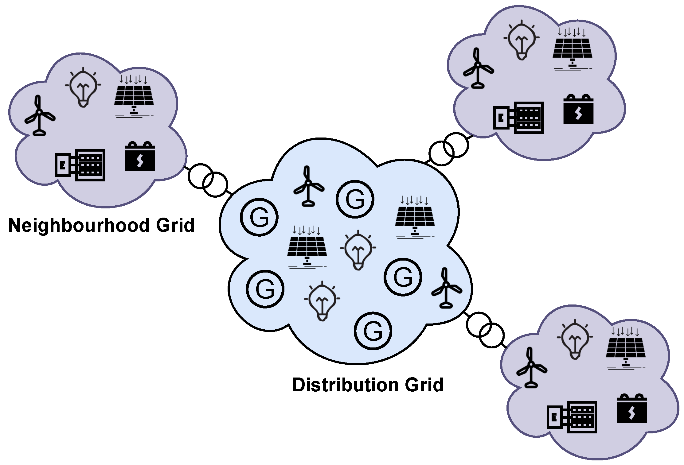
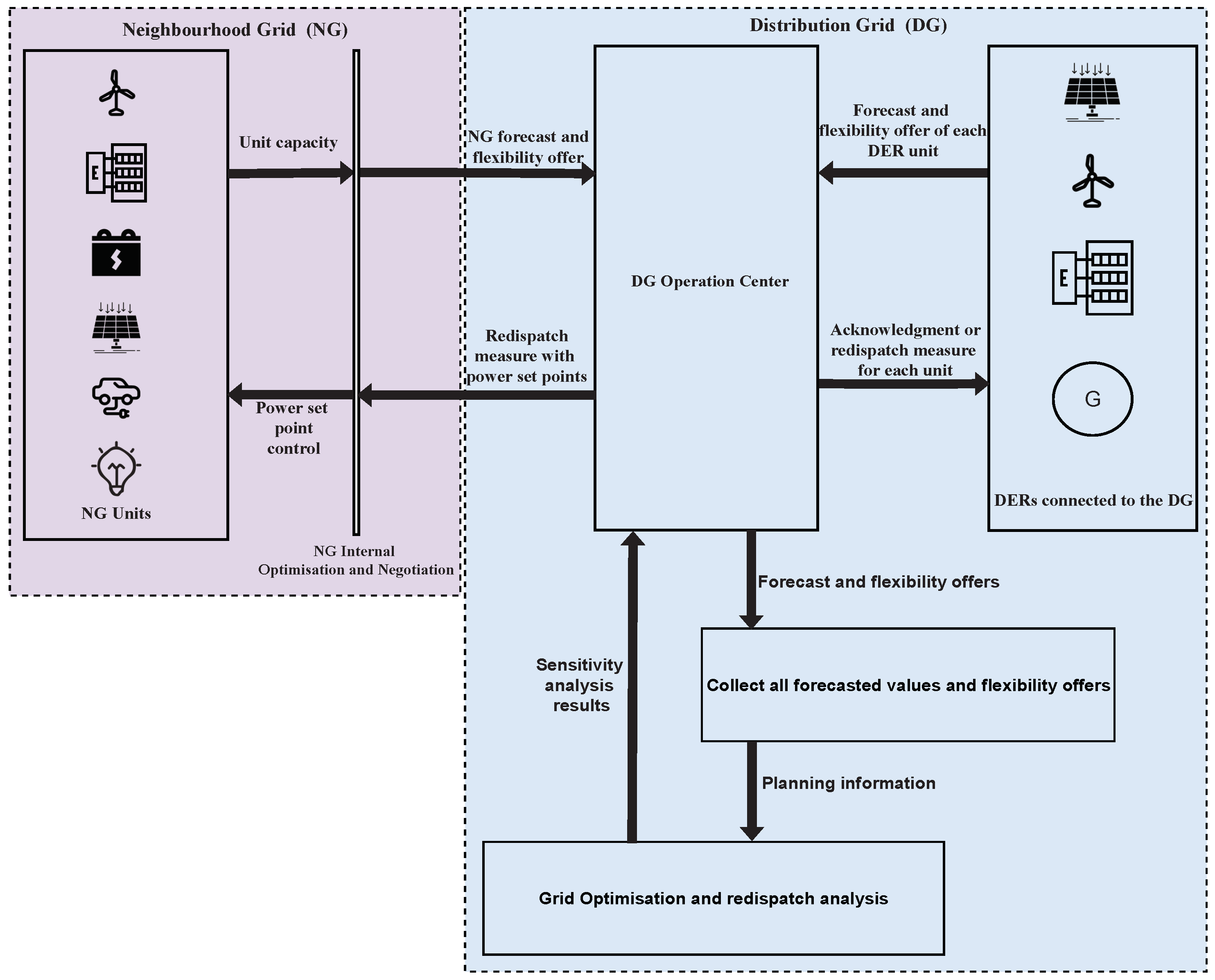
3.1. Scenario Description

The distribution grid (DG) represents the infrastructure with consumers, generators (G), and distributed energy resources (DERs). It is connected to several neighbourhood grids composed of DER units, loads, and electric vehicle charging stations. The neighbourhood grids (NG) and the distribution grid are connected through a dedicated transformer for each neighbourhood grid. In this study, the higher voltage bus bar of the transformer is the connection point between both grids, as shown in Figure 2. This connection point is used by the neighbourhood grid to deliver surplus energy to the distribution grid or to receive energy in case their resources are unavailable due to weather conditions or equipment constraints. Further, at this connection point, the aggregated flexibility resulting from the optimisation process in the lower-level is forecasted and offered to the distribution grid operator (upper-level).
In addition to that, in order to comply with the current Redispatch 2.0 regulations, the DER units with a capacity > 100 kW, connected to the distribution grid, must submit their forecasted power production. The power production forecast is considered a flexibility offer since the Redispatch 2.0 supports curtailment decisions of that power, and it is assumed that each DER unit is willing to supply as much as it has available. Flexibility is forecasted for every time step (t) of a time frame T. The distribution grid operator uses all forecasted flexibility offers (from DER and/or from neighbourhood grids) to optimise its power grid. If a possible line congestion appears, in that time frame, the operator would optimise its grid and sets a maximum consumption or feed-in value in kW ( P s e t ) to the components that could contribute to avoid the grid congestion problem.
The distribution grid operator is considered to be the upper-level since the power grid optimisation decisions must be followed by the lower-level (neighbourhood grid). The upper-level optimisation problem is the leader’s problem (upper-level decision maker), and the lower-level optimisation problem is the follower’s problem (lower-level decision maker). Any decision taken by the distribution grid operator (upper-level) alters the internal decisions in the neighbourhood grid (lower-level). In addition to that at any given instance the lower-levels internal objectives must be fulfilled.
In our setting, the two optimisation problems are combined to form a bi-level, multi-objective optimisation problem where uncertainties are evident. Interactions between the distribution grid (upper-level) and the neighbourhood grid (lower-level) during operation are shown in Figure 3. The arrows represent the information flow among different processes. The DERs connected to the distribution grid (DG) send a forecast and a flexibility offer to the DG operation center. The neighbourhood grid (NG) does an internal negotiation and optimises the resources based on the capacities of the units and the state of the components (e.g., battery, CHP). The result of this internal negotiation is the flexibility offer to the DG operation center. The DG operation center receives all forecasts and flexibility offers, collects them and performs a load flow calculation of its power grid. In case of a grid congestion scenario, a grid optimisation and redispatch analysis is performed. The results of this load flow calculation provide optimal  P s e t  values for the specific DERs and/or neighbourhood grid, based on a sensitivity analysis. This local sensitivity analysis assesses the effect of a single parameter  P s e t  value at a time t while holding all other parameters constant (the results of the load flow). Note that the present study only considers a single neighbourhood grid connected to the distribution grid.

3.2. Distribution Grid

The distribution grid used to represent the upper-level is a section of a real distribution grid topology composed of 13 substations connected with a total of 34 main feeders between them. One substation is selected in which 2 transformers reduce the voltage from an external feed into a medium voltage level (110 kV/22 kV) at 55 MVA and 50 Hz. A load flow calculation is performed on this grid considering an external grid that is able to provide or receive the power in the selected substation. During maximum demand, the external grid delivers 37.2 MW and 2.4 MVar to our selected substation, and under maximum generation, the external grid delivers −91.6 MW and 6.1 MVar to the same selected substation. This means that for the maximum generation cases, the high voltage level (external grid) is receiving power. The neighbourhood grid is connected to one of the feeders in the medium voltage (22 kV) in the selected substation, in which other DER units and loads are connected. In this paper, it is assumed that all DER units as well as the neighbourhood grid are subject to redispatch measures.
In the following sections, the mathematical formulation of the upper-level problem is provided. This formulation is the foundation to apply bi-level optimisation algorithms to the described problem where the design of the model for the distribution grid is represented in terms of model parameters, decision variables, objectives, and constraints.

3.2.1. Model Parameters

Following model parameters are considered for the distribution grid modelling.
(i)
t N : is defined as the time step. The time step is usually 15 min. This parameter is the same also for the neighbourhood grid.
(ii)
T N : is defined as the period of time for the entire calculation. The redispatch process runs for a duration T T = 32.5  h (this is the same for the neighbourhood grid [22,23]).
(iii)
N g r i d , t N : is defined as the number of generators that have to comply with a redispatch measurement at time t for every  t = 1 , , T .
(iv)
N L i n e s N : represents the number of lines.
(v)
R i R : is a parameter that represents the resistance of the line.
(vi)
N N R N : represents the number of non-renewable generators.
(vii)
C CO 2 R : is the cost of  C O 2 .
(viii)
C R e d i s p a t c h i R : is the Redispatch cost for the ith generator.

3.2.2. Decision Variables

The decision variable under consideration for the distribution grid are:
(i)
P G i R : is defined as the power generated by the ith generator that could be subject to redispatch measures at time t for  i = 1 , , N g r i d , where  N g r i d  represents the number of generators as defined in Section 3.2.1.
(ii)
P L o s s i R : represents the power loss in the ith line, for every time t. This is a calculation based on the results of the power flow.
(iii)
E N R i R : represents the energy generated by the ith non-renewable energy source.

3.2.3. Objectives

The distribution grid in this study is optimised considering the following three objectives:
(i)
Minimise real power losses.
min O b j 1 U = i = 1 N L i n e s P L o s s i
where  N L i n e s N  represents number of lines and  P L o s s i R , represents the loss in the ith line. The  P L o s s i  is calculated using Ohm’s law as follows:
P L o s s i = I i 2 ( t ) × R i
where  R i R  is the resistance of the line, which is a property of the type of cable or conductor used for every ith line.
(ii)
Minimise CO 2  cost.
min O b j 2 U = i = 1 N N R C O 2 i × E N R i
C O 2 R , is the cost of C O 2 for the generation of a unit of real power of each non-renewable generator and  E N R i R , represents the energy generated by the ith non-renewable energy source. It is considered that the energy produced externally (generated by the slack bus) is provided from non-renewable sources for  i = 1 , , N N R .
(iii)
Minimise Redispatch costs.
min O b j 3 U = i = 1 N g r i d C R e d i s p a t c h i × P G r e d i s p a t c h i
where  N g r i d N , represents the number of generators,  C R e d i s p a t c h i R  is the Redispatch cost for the ith generator. The Redispatch cost is non-time dependent. Note that it is possible to to change Redispatch cost to dynamic values.  P G r e d i s p a t c h i R , represents the power that could not be generated due to Redispatch measures. It is defined as followed:
i = 1 N g r i d P G r e d i s p a t c h i = P G o f f e r e d i P G i
where  P G o f f e r e d i R  represents the real power offered by every generator, connected to the distribution grid operator.  P G o f f e r e d i  is a function of the resources for each DER at time t for  t = 1 , , T . For example, for photovoltaic systems  P G o f f e r e d i  is a function of the solar irradiance and for wind turbines, it is a function of the wind speed. For other non-weather dependent generators,  P G o f f e r e d i  represents the maximum capacity of the unit for  t = 1 , , T , when the other unit constrains are satisfied, which is described further in Section 3.3. Note that For the neighbourhood grids,  P G o f f e r e d i  is a result of the lower-level optimisation.  P G i R , represents the real power generated by the ith generator at time t for  t = 1 , , T .

3.2.4. Constraints

The upper-level optimisation problem is constrained under two types of constraints which are represented as follows:
(i)
Equality constraints
i = 1 N G P G i + j = 1 N L P L j + P S = 0
i = 1 N G Q G i + j = 1 N L Q L j + Q S = 0
where  P G i 0  and  Q G i 0 , respectively, denote the active and reactive power generated by the ith generator,  P L j 0  and  Q L j 0 , respectively, denote the active and reactive power consumed by the jth load and  P S R  and  Q S R  denote the active and reactive power generated/consumed by the slack bus.
(ii)
Inequality constraints
P G , M i n i P G i P G , M a x i
Q G , M i n i Q G i Q G , M a x i
V M i n i V i V M a x i
T j M i n T j T j M a x
L F k L F k M a x
where  P G , M i n i P G , M a x i Q G , M i n i Q G , M a x i , respectively, denote the minimum and the maximum active and reactive power limits of the ith generator,  V i V M i n i V M a x i , respectively, denote the voltage of the ith node and its minimum and maximum limits,  T j T j M i n T j M a x , respectively, denote the tap setting of the jth transformer and its minimum and maximum limits and  L F k L F k M a x , respectively, denote the line flow of the kth line and its maximum limit.

3.3. Neighbourhood Grid

For the neighbourhood grid, it is assumed that energy generated from all renewable sources is generated at a zero cost. The decision between whether to store energy in a battery, to produce energy using a combined heat and power (CHP) unit, or to shift load from the e-vehicles charging station is taken based on the results of the optimisation. In order to adhere to Redispatch 2.0, resource optimisation is also considered an objective. Further, a sensitivity analysis is carried out to find out the in-feed location which determines the degree of flexibility that the distribution grid can use from the neighbourhood grid or from any other DER unit connected to it.
This smart neighbourhood was built to supply thermal, electricity, and mobility needs with its own resources for 230 households in 13,000 m 2 . The testing scenario considered in this study is composed of a photovoltaic (PV) plant, a wind turbine and battery storage to cater for the electrical demand. In addition to that, a CHP unit which has a thermal storage tank is incorporated to supply thermal demand and 20 electric charging stations are incorporated to supply the e-mobility demand.
In the following sections, the mathematical formulation of the lower-level problem is provided. This formulation is the foundation to apply bi-level optimisation algorithms to the described problem where the design of the model for the neighbourhood grid is represented in terms of model parameters, decision variables, objectives, and constraints.

3.3.1. Model Parameters

Following model parameters are considered for the neighbourhood grid modelling.
(i)
n L N : number of household loads.
(ii)
n P V N : number of photovoltaic generators.
(iii)
n W i n d N : number of wind generators.
(iv)
p L , t i R p L , t i 0  power of the ith load at time t on households.
(v)
p P V , t i R p P V , t i 0  PV power of ith PV at time t.
(vi)
p W i n d , t i R p W i n d , t i 0 :  power of the wind generator at time t.
(vii)
C C O 2 R  is the cost of C O 2 emission to generate unit energy.
(viii)
α ( 0 , 1 ) :  minimum state of charge allowed.
(ix)
β ( 0 , 1 ) :  maximum state of charge allowed ( α < β ).
(x)
M C H P R : maximum energy generated by the CHP unit.
(xi)
Δ > 0 :  sampling time (or time step).
(xii)
F o r e c a s t E m o b , t R F o r e c a s t E m o b , t 0 :  Forecast of the energy for the electric vehicles needed at time t.
(xiii)
S o C ( t ) R : state of charge of the battery at time t.
(xiv)
E C h p ( t ) R : energy produced by the CHP unit at time t.

3.3.2. Decision Variables

The decision variable under consideration for the neighbourhood grid are:
(i)
F C h p , t R : flexibility power offer from CHP at time t.
(ii)
F B a t , t R : flexibility power offer from Battery at time t.
(iii)
F E m o b , t R : flexibility power offer from e-mobility at time t.

3.3.3. Objectives

The neighbourhood grid considered in this study has the following objectives:
(i)
Maximise self-consumption/minimise energy supply from the distribution grid.
O b j 1 L = min max t = 1 , , T i = 0 n L p L , t i i = 0 n P V p P V , t i j = 0 n W i n d p W i n d , t j ( F C h p , t + F B a t , t + F E m o b , t )
where  n L  and  n G , respectively, denote the number of loads and generators,  p L i  denotes the power of the ith load,  p W i n d , t j  and  p P V , t i , respectively, denote the power generated by ith PV plant and jth wind power plant. Further,  F C h p , t F B a t , t , and  F E m o b , t , denote the flexibilities that are offered to the distribution grid by the neighbourhood grid using the CHP unit, battery storage and electric vehicle (EV) charging, respectively.
(ii)
Maximise flexibility offers for Redispatch 2.0.
O b j 2 L = max t = 1 T ( F C h p , t + F B a t , t + F E m o b , t )
where  F t  denotes the flexibility offered at time t and T denotes the Redispatch 2.0 time horizon which is usually  32.5  h.
(iii)
Minimise  C O 2  emissions.
O b j 3 L = min C C O 2 t = 1 T F C h p , t
Note that the only source of  C O 2  emissions is the CHP unit. Hence it is assumed that the cost of  C O 2  is proportional to the use of the CHP unit to offer flexibility.

3.3.4. Constraints

The lower-level optimisation problem is constrained as follows:
(i)
Energy produced by the CHP unit is fed into the neighbourhood grid.
0 F C h p , t M C H P t = 1 , , T .
where  M C H P  is the maximum power generated by the CHP. The dynamics of the CHP can be represented as:
E C h p ( t + 1 ) = F ( E C h p ( t ) , F C h p , t )
where  E C h p  represents the energy produced by the CHP unit.
(ii)
The e-mobility flexibilities are considered as load shifting, therefore the aggregated flexibility offered over the entire period is 0 so that the load equals the forecast by the end of the period T.
t = 1 T F E m o b , t = 0
(iii)
Energy supplied/consumed by battery storage.
t = 1 , , T : α M S o C ( t ) × M t × F B a t , t β M & α S o C ( t ) β
S o C ( t + 1 ) = S o C ( t ) F B a t , t M Δ
where M is the capacity of the battery,  S o C ( t )  is the state of charge of the battery,  α  and  β  are minimum and maximum state of charge (SoC) limits and  t × F B a t , t  represents the energy offer as a flexibility for that time period.
Further,  F C H P , t  and  F B a t , t  are modelled as dynamical systems and are represented using ordinary differential equations (ODEs). It is worth noting that the ODEs of the CHP and battery storage are also constraints for the neighbourhood grid (lower-level) optimisation problem.

4. Solution Approach

In the previous section, the problem was formulated. In this section, the two selected solution approaches are explained. First, the centralised approach with a performance-optimised software package to solve bi-level optimisation problems is presented. After that, a decentralised multi-agent based approach is discussed.

4.1. Centralised Approach

The main goal of the centralised approach is to model the distribution grid (DG) and neighbourhood grid (NG) as a multi-objective bi-level optimisation problem and to solve it using sequential quadratic programming (SQP) procedures. During the modelling process, the distribution grid and the neighbourhood grid are considered separately. Note that for the distribution grid, effects such as changes in voltage with respect to change of loads are negligible and thus modelled as a static network using single-phase equivalent circuit diagrams. This is a fair assumption given the size and capacity of the distribution grid. The static equations that represent the distribution grid are transformed into constraints of an optimisation problem to make it possible to optimise individual variables in the network. Reformulation of the complex-valued system of equations into the real-valued constraints, and automatic calculation of the derivatives and their structures are implemented.
However, in the neighbourhood grid, many temporal processes such as combined heat and power (CHP) units, and battery storage that constitute importance in optimisation, are present. In contrast to the distribution grid, the dynamic effects during consumption and generation are also considered on the basis of a time series. A dynamic model that is capable of mapping these processes is developed. It serves as a basis for an optimal control problem (OCP). Algorithms are then developed to establish the mathematical model descriptions for the neighbourhood network. Different model approaches for the different components of a neighbourhood network is used (e.g., simplified difference models for dynamic storage, data-based models for generators such as PV systems). Besides the basic modelling approaches, the focus is also on the automated creation of models. Then a simplified illustration of a neighbourhood network is first created where all interrelations, especially the flexibility, are represented as continuous decision variables. However, for some components such as components that can only be switched binary (e.g., either on or off) this simplification is not realistic and leads to a mixed-integer problem. These models require a much higher computational effort to solve the optimisation problems. Therefore, the number of such components that is needed for a realistic model has to be further investigated.
These static and dynamic models are combined into one large optimisation problem where the overall model forms a differential-algebraic system and the different objectives of the respective grids form a multi-objective optimisation problem. Hence, the resulting optimisation problem contains two levels, the upper-level is the distribution grid and the lower-level is the neighbourhood grid. The distribution grid operator has the possibility to control the behaviour of the distribution level, but not the internal decisions in the lower-level (neighbourhood grid), thus this becomes a bi-level optimisation problem. The two algorithms for both levels can be different approaches. It is expected that this is numerically more efficient, but the use of the Karush–Kuhn–Tucker (KKT) conditions to replace the lower-level has theoretical disadvantages, since they are only necessary optimality conditions. This problem does not occur with this approach. However, it is numerically very complex, especially for higher-dimensional problems. Therefore, an iterative combination of both algorithms is investigated in order to combine the respective advantages to a heuristic algorithm.
In order to solve this software package WORHP (https://worhp.de) developed by the Center for Industrial Mathematics, University of Bremen is used. WORHP is capable of solving high-dimensional, nonlinear optimisation problems using a KKT approach [42]. For this purpose, the bi-level problem is transformed into a KKT formulation and thus formulated as a continuous non-linear optimisation problem and is solved using WORHP. In order to increase efficiency, methods of structure utilisation (at the derivation level) and parallelisation strategies are also being investigated and results must be analysed with regard to solution quality, robustness and efficiency. One of the few existing numerical methods of multi-criteria (multi-objective), bi-level optimisation uses the description of the allowable set as a solution set for a new multi-criteria optimisation problem [43]. The latter is then solved by scalarisation approaches, but an enormous number of sub-problems have to be solved. Therefore, clever parallelisation strategies have to be developed. Next, using parametric sensitivity analysis and the WORHP Zen tool [44], the sensitivities of the individual disturbance variables can be automatically calculated. By also considering or estimating the possible ranges of interference for each variable, approximate corrections can be calculated using the parametric sensitivities. On this basis, an algorithm is implemented to automatically minimise the effects of uncertainties.

4.2. Decentralised Approach

The decentralised approach focuses on the neighbourhood grid and involves optimising an aggregated schedule for it. The previously set objectives are taken into account for this. The optimisation is implemented by the combinatorial optimisation heuristic for distributed agents (COHDA) (https://github.com/ambimanus/cohda), so that an operational management concept is possible that combines the advantages of multi-objective optimisation and a multi-agent approach. COHDA can be used to solve distributed combinatorial problems, e.g., to achieve a global target given individual local constraints. Thus, it can be used for a group of DERs pursuing a global target, with each unit choosing its own mode of operation to best achieve the global target [45]. For the present concept proposal, COHDA is implemented in a multi-agent system, which represents the neighbourhood grid. Each unit in the neighbourhood model is controlled by an agent. The agent knows the local constraints of the unit and can take them into account during the optimisation process. First, the agent creates a forecast for the power of its unit. Considering this forecast and the local constraints of the unit, it can then determine the flexibility that forms the basis for the optimisation. Then the agents inside the neighbourhood grid share their flexibility and their needs (load agents), determining the amount of flexibility that they could offer to the distribution grid agent for the following time period.
Due to the decentralised approach and the representation of each unit by an agent, individual unit constraints and local network constraints can be taken into account when implementing the overall objectives for the neighborhood grid. During optimisation, the agents consider the global objective and local penalties [45]. The current best solution from each agent’s point of view is communicated among other agents. Whenever an agent receives new information from others, it updates its own configuration and decides whether a better configuration can be found. For this decision, it takes its own local parameters into consideration as well. When an improvement is found concerning the global target, it informs the other agents about it by sharing its current configuration [45].
The described heuristic was extended to a multi-objective approach for the neighbourhood grid in order to take into account the objectives described in Section 3.3.3. For this multi-objective variant of COHDA, the principle of COHDA is combined with the S-metric selection evolutionary multi-objective algorithm (SMS-EMOA) to create a fully decentralised multi-objective algorithm, with which agents approximate a Pareto front. The implementation is based on [46].
For the simulation of different agents and their interactions, the co-simulation framework mosaik is used [47,48]. It offers various advantages including the integration of different models such as the distribution grid model and different components (agents) in the neighbourhood grid such as models for the wind power plant, the PV plant, household consumption and so on. The distribution grid model is provided in Power Factory from DigSilent. The optimisation within the neighbourhood grid is performed with COHDA and the agent system is implemented with mango (https://gitlab.com/mango-agents/mango). Whenever the agents found their operation schedule, it is communicated with the possible flexibility for the neighbourhood grid to the distribution grid operator model. This tool furthermore receives the planned power values and the possible flexibility from other plants of the distribution grid. Thus, it runs the load flow calculations for the distribution grid and determines, how the given power values could be adjusted according to the possible flexibility to avoid congestions. This information will be forwarded to the neighbourhood grid, where the agents responsible for the respective units make their adaptions.

4.3. Evaluation

This section proposes a method to evaluate the performance of the centralised and decentralised bi-level multi-criteria optimisation problems solving approaches. In particular, the solutions between multi-agent systems using the COHDA algorithm versus centralised solution obtained using WORHP. We select five Key Performance Indicators (KPIs) to evaluate the outcomes of the two approaches which are summerised in Table 1. These KPIs are selected to analyse the congestion solving capacity achieved by both approaches. In addition, it is of interest to investigate if the neighbourhood grid is self-sufficient or if it needs to curtail its production to support the upper level (distribution grid). Nevertheless, due to our multi-objective criteria in the neighbourhood grid, it is expected that any curtailment is chosen such that non-renewable sources such as the CHP units and the battery system are utilised first.
In addition, to evaluate the effectiveness of the solution, the internal optimisation of the lower-level (neighbourhood grid) needs to be able to comply with the maximum ( P s e t ) value from the upper-level. It is of particular interest to evaluate the extreme condition scenarios in this respect: maximum in-feed (power production) coming from DERs and the neighbourhood grids and maximum load condition in the distribution grid.
Another interesting aspect for future work will be evaluating the communication signals between the agents. How fast and accurate the communication between the real components can be, and how to avoid latency problems. For that, two scenarios can be considered: normal situations, i.e., perfect communication and extreme scenarios, i.e., poor communication bandwidth with high data loss.
Further, it would be interesting to investigate the possibility of incorporating dynamic pricing for the flexibility offers. The objective of maximising flexibility offer presented in Section 3.3.3 can be replaced by an economic goal in which the neighbourhood grid seeks to maximise profits by offering flexibility. One possible way of achieving this is by implementing flexibility markets where the price for the redispatch offer is decided dynamically based on the results of the internal optimisation.

5. Policy Implications

Grid operators seek to reduce losses and investment costs, while neighbourhood grid (NG) actors seek to maximise its profits. Neighbourhood grid can only achieve this by either consuming its own energy, or offering it as a flexibility service, as discussed in this paper. Nevertheless, the willingness of the neighbourhood grid actor to maximise its flexibility offer, can be different if a market mechanism is implemented.
Policy makers must decide if the flexibility offers should be paid based on costs or based on a market mechanisms. If a market mechanism for flexibilities is implemented, neighbourhood grid actor will need to consider a forecasted price for the flexibility offer. This introduces another objective to the lower-level problem.
O b j 4 L = max t = 1 T ( F t P f , t )
where  F t  denotes the flexibility offered at time t; T denotes the Redispatch 2.0 time horizon which is usually  32.5  h, and  P f , t  is the forecasted price at time t.

6. Conclusions

This paper presented the integration of neighbourhood grids to the German distribution grid as a bi-level, multi-objective optimisation problem that can be implemented to tackle congestion-related issues in distribution grids by using the flexibility of local resources. It is also discussed in this paper how to manage the resources in the neighbourhood grid to solve the problems associated with the fluctuating energy generation from renewable energy sources, which leads to less computational costs. In addition, the paper also proposed a set of objective functions for the bi-level optimisation problem (upper-level and lower-level) and two different approaches to solve them; the centralised approach and the decentralised approach.
In addition, we propose an extension of the redispatch measures to integrate locally optimised neighbourhood grids into the power grid in such a way that the optimisation goals of both grids are satisfied. The equations presented focus on the possibility that the aggregated flexibility coming from the neighbourhood grid can contribute to solve grid congestions in the distribution grid while fulfilling its own objectives.
Concerning optimisation solutions, the centralised approach requires knowing all the information of the components, including the ones in the neighbourhood grid. However, the operational status of the DER units inside the neighbourhood grid is usually unknown to the distribution grid operator. For this reason, the decentralised approach is probably closer to reality. Further work is to test these methods in real-time conditions. Another interesting topic for future research would be to investigate the uncertainty related to each DER unit and neighbourhood grid as a whole, due to weather dependencies. Furthermore, for the evaluation and comparison between both approaches, KPIs are implemented. The overall objective is to determine the effectiveness of the solution provide by the centralised and decentralised approaches. However, these performance metrics can be incorporated with metrics related to operational performance behaviour such as computational time for finding the solution space to asses the effectiveness of the proposed two algorithms.

Author Contributions

Conceptualisation, R.R.A., C.W., E.F. and T.B.; Methodology, R.R.A., C.W., E.F. and T.B.; Investigation, R.R.A., C.W., E.F. and T.B.; Writing—Original Draft Preparation, R.R.A., C.W., E.F. and T.B.; Writing—Review & Editing, R.R.A., C.W., E.F. and T.B.; Supervision, S.L. and C.B.; Project Administration, S.L. and C.B.; Funding Acquisition, S.L. and C.B. All authors have read and agreed to the published version of the manuscript.

Funding

This research was funded by the Bundesministerium für Wirtschaft und Klimaschutz (BMWK) [grant number 03EI4013C]. The APC was funded by German Aerospace Centre (DLR).

Data Availability Statement

There is no data associated with the article.

Conflicts of Interest

The authors declare no conflict of interest.

Nomenclature

AbbreviationMeaning
COHDACombinatorial Optimisation Heuristic for Distributed Agents
CHPCombined Heat and Power
DERsDistributed Energy Resources
DGDistribution Grid
DSODistributed System Operator
FFlexibility
GGenerators
KPIsKey Performance Indicators
NGNeighbourhood Grid
OCPOptimal Control Problem
PVPhotovoltaic
SQPSequential Quadratic Programming
SoCState of Charge

References

  1. Mishra, P.; Vidyarthi, A.; Siano, P. Guest Editorial: Security and Privacy for Cloud-Assisted Internet of Things (IoT) and Smart Grid. IEEE Trans. Ind. Inform. 2022, 18, 4966–4968. [Google Scholar] [CrossRef]
  2. Chaudhry, S.A.; Nebhan, J.; Yahya, K.; Al-Turjman, F. A Privacy Enhanced Authentication Scheme for Securing Smart Grid Infrastructure. IEEE Trans. Ind. Inform. 2022, 18, 5000–5006. [Google Scholar] [CrossRef]
  3. Sanduleac, M.; Ciornei, V.I.; Toma, L.; Plamnescu, R.; Dumitrescu, A.M.; Albu, M. High Reporting Rate Smart Metering Data for Enhanced Grid Monitoring and Services for Energy Communities. IEEE Trans. Ind. Inform. 2022, 18, 4039–4048. [Google Scholar] [CrossRef]
  4. Kouvelas, N.; Prasad, R.V. Efficient Allocation of Harvested Energy at the Edge by Building a Tangible Micro-Grid—The Texas Case. IEEE Trans. Green Commun. Netw. 2021, 5, 94–105. [Google Scholar] [CrossRef]
  5. Kester, J. Conducting a smarter grid: Reflecting on the power and security behind smart grids with foucault. In Smart Grids from a Global Perspective: Bridging Old and New Energy Systems; Springer: Berlin/Heidelberg, Germany, 2016; pp. 197–213. [Google Scholar]
  6. Mullen, S.; Onsongo, G. Decentralized agent-based underfrequency load shedding. Integr. Comput. Aided Eng. 2010, 17, 321–329. [Google Scholar] [CrossRef]
  7. Frank, S.; Steponavice, I.; Rebennack, S. Optimal power flow: A bibliographic survey I Formulations and deterministic methods. Energy Syst. 2012, 3, 221–258. [Google Scholar] [CrossRef]
  8. Kumar, Y.; Devabhaktuni, V.K.; Vemuru, S. Comparison of power system simulation tools with load flow study cases. IEEE Int. Conf. Electro Inf. Technol. 2015, 2015, 290–294. [Google Scholar]
  9. Kundur, P.; Balu, N.J.; Lauby, M. Power System Stability and Control; McGraw-Hill: New York, NY, USA, 1994. [Google Scholar]
  10. Wanigasekara, C.; Swain, A.; Almakhles, D.; Zhou, L. Design of Delta–Sigma-Based PID Controller for Networked Wind Energy Conversion Systems. IEEE Trans. Ind. Appl. 2022, 58, 879–889. [Google Scholar] [CrossRef]
  11. Kashyap, M.; Kansal, S.; Verma, R. Sizing and Allocation of DGs in A Passive Distribution Network Under Various Loading Scenarios. Electr. Power Syst. Res. 2022, 209, 108046. [Google Scholar] [CrossRef]
  12. Alasvand Javadi, E.; Joorabian, M.; Barati, H. A bi-level optimization framework for resilience enhancement of electricity and natural gas networks with participation of energy hubs. Int. J. Electr. Power Energy Syst. 2022, 142, 108312. [Google Scholar] [CrossRef]
  13. Bracken, J.; Mcgill, J.T. Mathematical programs with optimization problems in constraints. Oper. Res. 1973, 21, 37–44. [Google Scholar] [CrossRef]
  14. Dempe, S. Foundations of Bilevel Programming; Springer Science & Business Media: Cham, Switzerland, 2002. [Google Scholar]
  15. Colson, B.; Marcotte, P.; Savard, G. An overview of bilevel optimization. Ann. Oper. Res. 2007, 153, 235–256. [Google Scholar] [CrossRef]
  16. Sinha, A.; Malo, P.; Deb, K. Towards understanding bilevel multi-objective optimization with deterministic lower level decisions. In Proceedings of the International Conference on Evolutionary Multi-Criterion Optimization, Guimaraes, Portugal, 29 March–1 April 2015; pp. 426–443. [Google Scholar]
  17. Thirugnanam, K.; El Moursi, M.S.; Khadkikar, V.; Zeineldin, H.H.; Hosani, M.A. Energy Management Strategy of a Reconfigurable Grid-Tied Hybrid AC/DC Microgrid for Commercial Building Applications. IEEE Trans. Smart Grid 2022, 13, 1720–1738. [Google Scholar] [CrossRef]
  18. Tziovani, L.; Hadjidemetriou, L.; Kolios, P.; Astolfi, A.; Kyriakides, E.; Timotheou, S. Energy Management and Control of Photovoltaic and Storage Systems in Active Distribution Grids. IEEE Trans. Power Syst. 2022, 37, 1956–1968. [Google Scholar] [CrossRef]
  19. Ehrgott, M. Multicriteria Optimization; Springer Science & Business Media: Cham, Switzerland, 2005; Volume 491. [Google Scholar]
  20. Eichfelder, G. Adaptive Scalarization Methods in Multiobjective Optimization; Springer: Berlin/Heidelberg, Germany, 2008. [Google Scholar]
  21. Miettinen, K. Nonlinear Multiobjective Optimization; Springer Science & Business Media: Cham, Switzerland, 2012; Volume 12. [Google Scholar]
  22. Kreutziger, M.; Wende-von Berg, S.; Krahmer, S.; Schegner, P. Provision of reactive power from wide area distribution grids—Practical implementation in a field test. Elektrotech. Informationstech. 2022, 139, 65–72. [Google Scholar] [CrossRef]
  23. Linnemann, M. Redispatch 2.0 challenge: Improved airbag for grid stability. BWK Energ. Fachmag. 2021, 73, 12–13. [Google Scholar] [CrossRef]
  24. Wehkamp, S.; Schmeling, L.; Vorspel, L.; Roelcke, F.; Windmeier, K.L. District Energy Systems: Challenges and New Tools for Planning and Evaluation. Energies 2020, 13, 2967. [Google Scholar] [CrossRef]
  25. Poplavskaya, K.; Totschnig, G.; Leimgruber, F.; Doorman, G.; Etienne, G.; De Vries, L. Integration of day-ahead market and redispatch to increase cross-border exchanges in the European electricity market. Appl. Energy 2020, 278, 115669. [Google Scholar] [CrossRef]
  26. De Oliveira, R.; de Oliveira, L.W.; de Oliveira, E.J. Optimization Approach for Planning Soft Open Points in a MV-Distribution System to Maximize the Hosting Capacity. Energies 2023, 16, 1035. [Google Scholar] [CrossRef]
  27. Ferdowsi, A.; DehghanChenary, M.; Jolai, F.; Tavakkoli-Moghaddam, R. Toward unraveling multi-objective optimization problems: A hybrid approach for solving a novel facility location problem. TechRxiv, 2022; preprint. [Google Scholar]
  28. Abdelmalak, M.; Benidris, M. Proactive generation redispatch strategy considering unavailability of renewable energy sources during hurricanes. In Proceedings of the 2021 IEEE Industry Applications Society Annual Meeting (IAS), Vancouver, BC, Canada, 10–14 October 2021; pp. 1–6. [Google Scholar]
  29. Hu, D.; Wang, T. Optimizing Power Demand Side Response Strategy: A Study Based on Double Master &ndash;Slave Game Model of Multi-Objective Multi-Universe Optimization. Energies 2023, 16, 4009. [Google Scholar]
  30. Grisales-Noreña, L.F.; Montoya, O.D.; Perea-Moreno, A.J. Optimal Integration of Battery Systems in Grid-Connected Networks for Reducing Energy Losses and CO2 Emissions. Mathematics 2023, 11, 1604. [Google Scholar] [CrossRef]
  31. Zhang, Y.; Song, X.; Li, Y.; Zeng, Z.; Yong, C.; Sidorov, D.; Lv, X. Two-stage active and reactive power coordinated optimal dispatch for active distribution network considering load flexibility. Energies 2020, 13, 5922. [Google Scholar] [CrossRef]
  32. Rocha, R.; Silva, R.; Mello, J.; Faria, S.; Retorta, F.; Gouveia, C.; Villar, J. A Three-Stage Model to Manage Energy Communities, Share Benefits and Provide Local Grid Services. Energies 2023, 16, 1143. [Google Scholar] [CrossRef]
  33. Zatti, M.; Martelli, E.; Amaldi, E. A three-stage stochastic optimization model for the design of smart energy districts under uncertainty. In Computer Aided Process Engineering; Elsevier: Amsterdam, The Netherlands, 2017; Volume 40, pp. 2389–2394. [Google Scholar]
  34. Gadhi, N.; Hamdaoui, K.; El Idrissi, M. Optimality conditions for a multiobjective bilevel optimization problem involving set valued constraints. Optimization 2021, 70, 2013–2029. [Google Scholar] [CrossRef]
  35. Ashoornezhad, A.; Falaghi, H.; Hajizadeh, A.; Ramezani, M. A bi-level multistage distribution network expansion planning framework with the cooperation of residential private investors (A case study in Iran). IET Renew. Power Gener. 2023, 17, 1881–1898. [Google Scholar] [CrossRef]
  36. Echeverri Martínez, R. A bi-level multi-objective optimization model for the planning, design and operation of smart grid projects. Case study: An islanded microgrid. Int. J. Energy Econ. Policy 2020, 10, 325–341. [Google Scholar] [CrossRef]
  37. Ning, Y.; Chen, K.; Zhang, B.; Ding, T.; Guo, F.; Zhang, M. Energy conservation and emission reduction path selection in China: A simulation based on bi-level multi-objective optimization model. Energy Policy 2020, 137, 111116. [Google Scholar] [CrossRef]
  38. Stojiljković, M.M. Bi-level multi-objective fuzzy design optimization of energy supply systems aided by problem-specific heuristics. Energy 2017, 137, 1231–1251. [Google Scholar] [CrossRef]
  39. Luo, X.; Liu, Y.; Liu, X. Bi-level multi-objective optimization of design and subsidies for standalone hybrid renewable energy systems: A novel approach based on artificial neural network. J. Build. Eng. 2021, 41, 102744. [Google Scholar] [CrossRef]
  40. Haghifam, S.; Dadashi, M.; Zare, K.; Seyedi, H. Optimal operation of smart distribution networks in the presence of demand response aggregators and microgrid owners: A multi follower Bi-Level approach. Sustain. Cities Soc. 2020, 55, 102033. [Google Scholar] [CrossRef]
  41. Fateh, H.; Safari, A.; Bahramara, S. A bi-level optimization approach for optimal operation of distribution networks with retailers and micro-grids. J. Oper. Autom. Power Eng. 2020, 8, 15–21. [Google Scholar]
  42. Büskens, C.; Wassel, D. The ESA NLP Solver WORHP. In Modeling and Optimization in Space Engineering; Fasano, G., Pintér, J.D., Eds.; Springer: New York, NY, USA, 2013; Volume 73, pp. 85–110. [Google Scholar]
  43. Dell’Aere, A. Numerical Methods for the Solution of Bi-Level Multi-Objective Optimization Problems. Ph.D. Thesis, Universitaet Paderborn, Paderborn, Germany, 2008. [Google Scholar]
  44. Kuhlmann, R.; Geffken, S.; Büskens, C. WORHP Zen: Parametric Sensitivity Analysis for the Nonlinear Programming Solver WORHP. In Proceedings of the Operations Research Proceedings 2017, Berlin, Germany, 6–8 September 2017; Kliewer, N., Ehmke, J.F., Borndörfer, R., Eds.; Springer International Publishing: Cham, Switzerland, 2018; pp. 649–654. [Google Scholar]
  45. Hinrichs, C.; Lehnhoff, S.; Sonnenschein, M. COHDA: A combinatorial optimization heuristic for distributed agents. In Proceedings of the International Conference on Agents and Artificial Intelligence, Barcelona, Spain, 15–18 February 2013; pp. 23–39. [Google Scholar]
  46. Bremer, J.; Lehnhoff, S. Towards fully decentralized multi-objective energy scheduling. In Proceedings of the 2019 Federated Conference on Computer Science and Information Systems (FedCSIS), Leipzig, Germany, 1–4 September 2019; pp. 193–201. [Google Scholar]
  47. Steinbrink, C.; Blank-Babazadeh, M.; El-Ama, A.; Holly, S.; Lüers, B.; Nebel-Wenner, M.; Ramírez Acosta, R.; Raub, T.; Schwarz, J.S.; Stark, S.; et al. CPES Testing with mosaik: Co-Simulation Planning, Execution and Analysis. Appl. Sci. 2019, 9, 923. [Google Scholar] [CrossRef]
  48. Ofenloch, A.; Schwarz, J.S.; Tolk, D.; Brandt, T.; Eilers, R.; Ramirez, R.; Raub, T.; Lehnhoff, S. MOSAIK 3.0: Combining Time-Stepped and Discrete Event Simulation. In Proceedings of the 2022 Open Source Modelling and Simulation of Energy Systems (OSMSES), Aachen, Germany, 4–5 April 2022; pp. 1–5. [Google Scholar]
  49. Brazier, R.; De Luca, E.; de Wit, P.; Eklund, H.; Gimeno, C.; Herbretau, S.; Zawadska, K. Smart Grid Key Performance Indicators: A DSO Perspective. 2022. Available online: https://cdn.eurelectric.org/media/5272/smart_grid_key_performance_indicators__a_dso_perspective-2021-030-0129-01-e-h-B85F16BF.pdf (accessed on 1 April 2023).
  50. Okwuibe, G.C.; Gazafroudi, A.S.; Hambridge, S.; Dietrich, C.; Trbovich, A.; Shafie-khah, M.; Tzscheutschler, P.; Hamacher, T. Evaluation of Hierarchical, Multi-Agent, Community-Based, Local Energy Markets Based on Key Performance Indicators. Energies 2022, 15, 3575. [Google Scholar] [CrossRef]
  51. Harder, W.J. Key Performance Indicators for Smart Grids Master Thesis on Performance Measurement for Smart Grids. Master’s Thesis, University of Twente, Enschede, The Netherlands, 2017. [Google Scholar]
  52. Vita, V.; Christodoulou, C.; Zafeiropoulos, I.; Gonos, I.; Asprou, M.; Kyriakides, E. Evaluating the flexibility benefits of smart grid innovations in transmission networks. Appl. Sci. 2021, 11, 10692. [Google Scholar] [CrossRef]
Figure 1. Consumers, and distributed energy resources (DERs).
Energies 16 04319 g001
Figure 2. Representation of a distribution grid, with loads, generators (G) and DERs and neighbourhood grids.
Energies 16 04319 g002
Figure 3. Integration and interaction between the neighbourhood grid and the distribution grid.
Energies 16 04319 g003
Table 1. Key Performance Indicators.
Key Performance IndicatorMeaningSource
Activation rate of Redispatch to avoid grid congestions from the DGs perspectiveAmount of activations needed to avoid grid congestionsPresent Paper
Congestion solving capabilityPerformance in using distributed system operator (DSO) assets, DER’s and neighbourhood grids to execute congestion solving and percentage reduction of overloaded lines using the flexibility[49]
Community self-sufficiencyPercentage of electricity demanded by the local community agents that is produced within the community[50]
Demand flexibilityThe amount of load that can be shifted temporally at each time step[51]
Degree of curtailmentPercentage of curtailment from the generation[52]
Disclaimer/Publisher’s Note: The statements, opinions and data contained in all publications are solely those of the individual author(s) and contributor(s) and not of MDPI and/or the editor(s). MDPI and/or the editor(s) disclaim responsibility for any injury to people or property resulting from any ideas, methods, instructions or products referred to in the content.

