Improved Prediction of the Higher Heating Value of Biomass Using an Artificial Neural Network Model Based on the Selection of Input Parameters

Abstract

Recently, biomass has become an increasingly widely used energy resource. The problem with the use of biomass is its variable composition. The most important property that determines the energy content and thus the performance of fuels such as biomass is the heating value (HHV). This paper focuses on selecting the optimal number of input variables using linear regression (LR) and the multivariate adaptive regression splines approach (MARS) to create an artificial neural network model for predicting the heating value of selected biomass. The MARS model selected the input data better than the LR model. The best modeling results were obtained for a network with three input neurons and nine neurons in the hidden layer. This was confirmed by a high correlation coefficient of 0.98. The obtained results show that artificial neural network (ANN) models are effective in predicting the calorific value of woody and field biomass, and can be considered a worthy simulation model for use in selecting biomass feedstocks and their blends for renewable fuel applications.

1. Introduction

The primary sources for conventional power generation are fossil fuels, such as coal, oil, and natural gas. Fossil fuel resources are being depleted; they also contaminate the environment with the products of their combustion: particulate matter, sulfur, nitrogen, and carbon oxides. Moreover, the unstable situation in the fuel market has prompted countries to become independent from raw material suppliers and produce energy on their own.

To reduce the rate of consumption of fossil fuels, renewable energy sources are used. These sources are inexhaustible and environmentally friendly. Biomass has the greatest significance in the fuel and energy balance due to its availability, as well as expected benefits for the environment and the economy of local communities. Biomass includes various types of agricultural and forest products, as well as residues from the wood processing industry, and it is used to generate electricity, heat, and transport fuels.

According to Directive 2009/28/EC of the European Parliament and of the Council of 23 April 2009 on the promotion of the use of energy from renewable sources (and amending and subsequently repealing Directives 2001/77/EC and 2003/30/EC), biomass denotes the biodegradable fraction of products, wastes, or residues of biological origin from agriculture (including plant and animal matter), forestry, and related industries, including fisheries and aquaculture, as well as the biodegradable fraction of industrial and municipal waste [1]. The energy from biomass can come from various processes: thermochemical (combustion, gasification, and pyrolysis), biological (anaerobic digestion and fermentation), or chemical (esterification). Currently, there is growing interest in biomass as a solid fuel, as its combustion produces steam for use in electricity generation, whereas its gasification produces combustible gas and syngas.

Compared with conventional fuels, biomass contains significantly more oxygen in the chemical bond structures, resulting in lower energy concentration per unit mass (energy density). Its negative characteristics include large variations in chemical composition (nitrogen, chlorine, alkali) and water content, the tendency to form tars, and an ash melting point [2,3,4]. The high heterogeneity and variability of biomass characteristics make it difficult to develop and adopt common test methods (standardization, normalization) for basic characteristics, such as the higher heating value (HHV). HHV is of key importance for the design and operation of biomass combustion systems. This property determines the efficiency of the thermochemical conversion of biomass to energy; the potential energy content of biomass must be known [5]. The HHV of fuel is equal to the amount of heat released after the complete combustion of a unit mass of fuel, taking into account the enthalpy of condensation of liquid water as a product of combustion under normal conditions. The fuels with higher HHV will have the highest possible energy production [6]. The HHV of biomass can be experimentally evaluated using an adiabatic oxygen bomb calorimeter, which is a simple and accurate method of measuring the changes between reactants and enthalpy of products.

Despite its simplicity, experimental analysis of HHV is not always possible [7]. Therefore, many empirical models that correlate the elemental composition (carbon (C), hydrogen (H), nitrogen (N), oxygen (O), sulfur (S)) of biomass, and HHV have been developed [8,9,10,11].

Most empirical models apply either to a single feedstock or to proximate and ultimate analysis data. The HHV values of biomass are strongly dependent on the physical and chemical properties of the biomass, climatic conditions, and the soil on which the biomass is grown. This variable composition of biomass forces the development of models to reflect different HHV values.

Several researchers have used statistical techniques and machine learning to successfully “predict” HHV. Essentially, the goal of these techniques was the same; namely, to predict the HHV values of various biomass materials as accurately as possible. Discriminant analysis and linear regression are the two most commonly used data mining techniques to construct HHV models. These techniques are good when the relationship between variables is linear. However, the relationship between the elemental composition of biomass and properties such as moisture content, ash quantity, volatile matter, and heat of combustion cannot be explained linearly. For this reason, the regression model may be insufficient for applications to biomass sample variables [12,13,14].

An alternative in modeling nonlinear variables is artificial neural networks (ANN). ANNs have many scientific and engineering applications, including process monitoring [15], waste volume prediction [16], and water quality prediction [17]. ANNs have been used for combustion modeling [18], energy consumption prediction [19], and prediction of oxidation stability of biodiesel derived from waste [20]. The application of ANNs for HHV prediction of solid fuels has been examined. Patel et al. (2007) used a non-linear ANN model to estimate the HHV of coals [21]. Huang et al. (2008) predicted straw HHV based on ash content [22]. Qian et al. (2018) developed a regression model to predict the HHV of poultry waste from proximate analysis [14]. With different inputs, including the chemical composition of biomass, physical, or physicochemical properties (such as density, moisture content, ash content, or volatile matter), ANN models are an efficient method to predict the HHV of biomass. ANN models give better results than linear models, such as regression [23,24].

ANN models have been criticized because of the overly long training process in designing the optimal network topology and the difficult-to-identify validity of potential input variables. The selection of an optimal and small number of input parameters while maintaining high model performance is a challenge in developing new ANN models for HHV forecasting. Moreover, there are few works that have found optimal input factors affecting HHV. A discriminant analysis, as well as linear regression and the multivariate adaptive regression splines approach (MARS), have been used to select input variables. Unlike discriminant analysis and linear regression, MARS demonstrates the ability to model complex relationships between data. Additionally, MARS can identify “important” independent variables with multiple variables; moreover, it does not require a long training process. The most important advantage of the MARS technique is the easy interpretation of the model, since it is the resulting model [25].

Aiming to improve the quality of neural network models predicting HHV, the purpose of the presented article is to select input variables using the multivariate adaptive regression splines approach (MARS) and linear regression (LR) to create a neural network (ANN) model predicting the heating value (HHV) of the biomass produced in Poland. Routine experimental data such as carbon, nitrogen, sulfur, hydrogen, moisture content (M), and volatile matter (V) of woody and field biomass typically found in Poland were used as input data. MARS and LR techniques will yield significant predictor variables, which will then serve as input data in the designed neural network model.

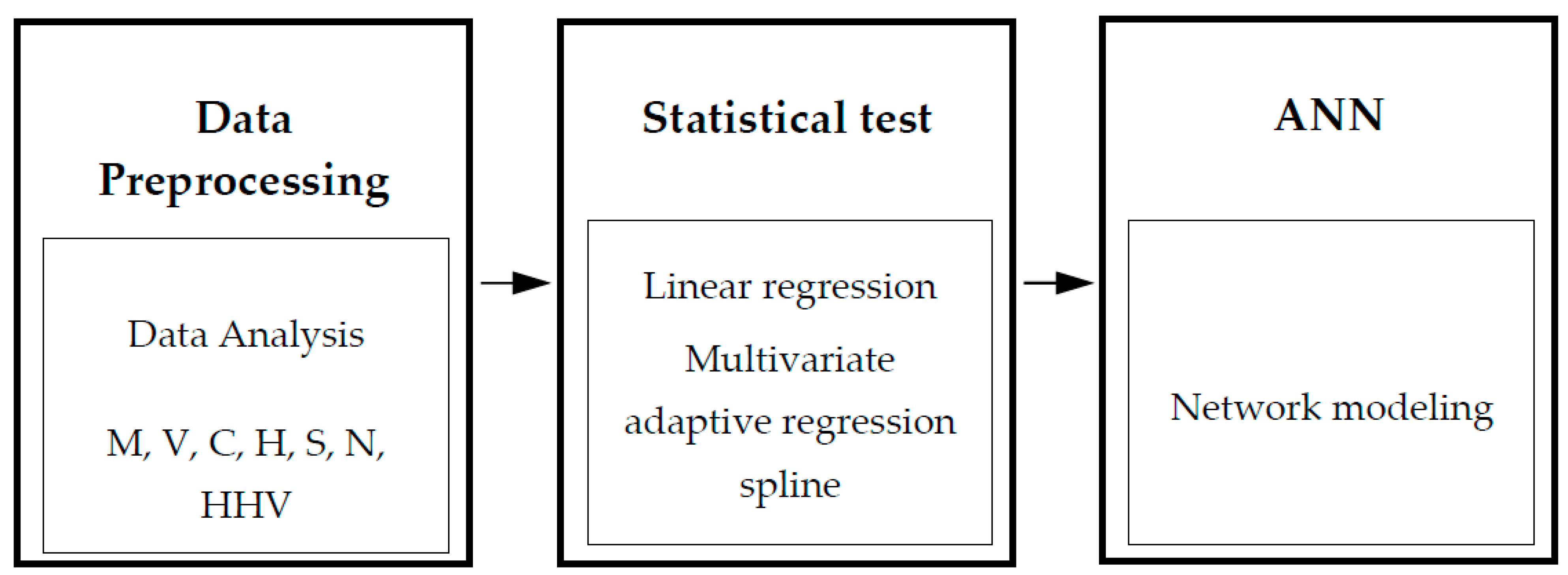
2. Materials and Methods

The research material consisted of the bark of oak, pine, hornbeam, alder, spruce, larch, and Douglas fir trees and waste from the field production of wheat, rape, oat, rye, triticale, barley, and maize straw. The biomass samples were collected from a farm in the village of Kobło (Poland).

Table 1. Testing methods employed in the biomass analysis.

Determined Parameters	Device	Standard
Moisture M (%)	Laboratory dryer	ISO 18134 (2017) [26]
Volatile matter V (%), ash content A (%)	FCF 2,5S electric muffle furnace made by Czylok with SM-946 electronic controller and temperature display (Warsaw, Poland)	ISO 18122 (2016) [27]
Determination of total carbon, hydrogen and nitrogen (%)	CHNS Flash EA 1112 Series Elemental Analyzer (Thermo Finnigan, Walthman, MA, USA)	ISO 16948 (2015) [28]
Higher heating value (HHV) (kJ/kg)	Mikado Calorimeter (Warsaw, Poland)	ISO 18125 (2015) [29]
The content of other combustible solid fractions FC (%)	FC was determined from the difference FC = 100-A-W-V	[30]

specifies the methods and standards followed in the biomass parameters testing.

An ANN model for HHV was built based on two methods of selecting input variables: linear regression and multivariate adaptive regression spline (MARS) [31]. The modeling process was carried out in Matlab 2022a and R (version 4.1.2, Vienna, Austria). The quality of the statistical model fit was tested using mean squared error (MSE)

$$\mathrm{MSE}=\frac{1}{\mathrm{n}}{\displaystyle \sum }_{\mathrm{n}=1}^{\mathrm{n}}{\left(\widehat{{\mathrm{y}}_{\mathrm{i}}}-{\mathrm{y}}_{\mathrm{i}}\right)}^2$$

(1)

together with root mean square error $\mathrm{RMSE}=\sqrt{\mathrm{MSE}}$, the determination coefficient (${\mathrm{R}}^2$)

$${\mathrm{R}}^2=\frac{{\sum }_{\mathrm{n}=1}^{\mathrm{n}}{\left(\widehat{{\mathrm{y}}_{\mathrm{i}}}-\overline{{\mathrm{y}}_{\mathrm{i}}}\right)}^2}{{\sum }_{\mathrm{n}=1}^{\mathrm{n}}{\left({\mathrm{y}}_{\mathrm{i}}-\overline{{\mathrm{y}}_{\mathrm{i}}}\right)}^2}.$$

(2)

and the mean absolute error ($\mathrm{MAE}$)

$$\mathrm{MAE}=\frac{1}{\mathrm{n}}{\displaystyle \sum }_{\mathrm{n}=1}^{\mathrm{n}}\left|\widehat{{\mathrm{y}}_{\mathrm{i}}}-{\mathrm{y}}_{\mathrm{i}}\right|$$

(3)

In the formulas above, $y_i$ and ${\widehat{y}}_i$denote the actual value of the i-th observation and the value predicted from the model, while $\overline{y_i}$ is the the sample mean. Recall that the lower the MSE, RMSE, and MAE, and the higher the R², the better the quality of the constructed model.

Let $X_1,X_2,\dots ,X_n$ and Y be input variables and dependent variable. The linear regression model

$$\mathrm{Y}={\mathsf{\alpha }}_0+{\mathsf{\alpha }}_1{\mathrm{X}}_1+{\mathsf{\alpha }}_2{\mathrm{X}}_2+\dots +{\mathsf{\alpha }}_{\mathrm{n}}{\mathrm{X}}_{\mathrm{n}},$$

(4)

is a convenient tool for selecting input variables, it allows understanding of the impact of individual variables on Y by model coefficients ${\alpha }_1,{\alpha }_2,\dots ,{\alpha }_n$. The following assumptions for linear regression model were verified: normality of the distribution of the residuals—Shapiro–Wilk test; homoscedasticity of the residuals—Breusch–Pagan test; absence of autocorrelation of the residuals—Durbin–Watson test; existence of outliers—Bonferroni outlier test.

Multivariate adaptive regression spline (MARS) is a nonparametric regression analysis method that is used to model nonlinear relationships and interactions. In the simplest form, the MARS model has the form

$$\mathrm{Y}={\mathsf{\alpha }}_0+{\mathsf{\alpha }}_1\cdot {\mathrm{h}}_1\left({\mathrm{X}}_{{\mathrm{i}}_1}\right)+{\mathsf{\alpha }}_2\cdot {\mathrm{h}}_2\left({\mathrm{X}}_{{\mathrm{i}}_2}\right)+\dots +{\mathsf{\alpha }}_{\mathrm{m}}\cdot {\mathrm{h}}_{\mathrm{m}}\left({\mathrm{X}}_{{\mathrm{i}}_{\mathrm{m}}}\right),$$

(5)

where $h_j\left(x\right)$, $j=1,2,\dots ,m$, is a hinge function equal to $\max \left(0,x-c_j\right)$ or $\max \left(0,c_j-x\right)$ (where $c_j$ is a constant, the cutpoint) and $i_1,i_2,\dots ,i_m\in \left\{1,2,\dots ,n\right\}$ (each independent variable used in the model can appear in more than one term). Max () is the maximum function, that is: for real numbers a, b, max(a,b) denotes the larger of a and b, i.e., max(a,b) = a if a > b and max(a,b) = b otherwise. The MARS model can also include terms representing interactions, being a product of some number of hinge functions. In order to use the MARS model as a tool for selecting input variables for the ANN model, only a basic model (without interaction terms) was considered in this study. The modeling process was carried out in the R environment using the Earth package [32]. The optimal model was determined using the generalized cross-validation method (backward pass). As a result, the optimal number of terms m in the model and the related most important independent variables used and cut points were found. These variables form the input for ANN model.

A network with one hidden layer was used to model ANN, in which the number of neurons ranged from 2 to 10. Three types of learning algorithms were tested: the Levenberg-Marquardt (L-M) algorithm, the Bayesian regularization algorithm (BR), and the Scaled conjugate gradient algorithm (SCG). Three algorithms were chosen on the basis of their performance. Although the Levenberg-Marquardt method is faster, it often uses more memory. As shown by an increase in the mean square error of the validation samples, training automatically stops when generalization no longer improves [33,34]. However, even if Bayesian regularization takes longer, it can produce good generalization for complicated, small, or difficult data sets. Training stops due to adaptive weight loss (regularization) [35,36]. On the other hand, the Scaled Conjugate Gradient Backpropagation technique uses less memory than the previous ones. When the generalization no longer improves, training stops automatically, as indicated by an increase in the mean square error of the validation samples [37,38]. The data set was divided in the proportion of 75% (training set): 25% (validation set), omitting the test set due to the small amount of input data [15]. The quality of the network was determined on the basis of qualitative indicators presented in

Table 2. Quality indicators used to evaluate the received networks.

Quality Indicator	Formula	Meaning of Symbols
Regression value R	$\mathrm{R}\left({\mathrm{y}}^{\prime },{ \mathrm{y}}^{*}\right)=\frac{\mathrm{cov}\left({\mathrm{y}}^{\prime },{ \mathrm{y}}^{*}\right)}{{\mathsf{\sigma }}_{{\mathrm{y}}^{\prime }}{\mathsf{\sigma }}_{{\mathrm{y}}^{*}}}, \mathrm{R}ϵ\langle 0,1\rangle$	σy′—standard deviation of reference values of HHV, σy*—standard deviation of predicted values HHV, yi is the actual value of HVV, $\widehat{{\mathrm{y}}_{\mathrm{i}}}$ denotes the value of the HVV for the i-th observation obtained from the model
Mean Squared Error (MSE)	$\mathrm{MSE}=\frac{1}{\mathrm{n}}{\displaystyle {\displaystyle \sum }_{\mathrm{n}=1}^{\mathrm{n}}}{\left(\widehat{{\mathrm{y}}_{\mathrm{i}}}-{\mathrm{y}}_{\mathrm{i}}\right)}^2$
Root Mean Square Error (RMSE)	$RMSE=\sqrt{\frac{{\sum }_{i=1}^n{\left(y_i-{\widehat{y}}_i\right)}^2}{n}}$
Mean Absolute Percentage Error (MAPE)	$MAPE=\frac{1}{n}{\displaystyle {\displaystyle \sum }_{i=1}^n}\left|\frac{y-y^{\prime } }{y}\right|$
Mean Absolute Error (MAE)	$MAE==\frac{1}{N}{\displaystyle {\displaystyle \sum }_{i=1}^N}\left(\left|y_i-{\widehat{y}}_i\right|\right)$

.

The methodology for the development of this research is shown in the flowchart below (Figure 1).

3. Results

3.1. Dataset

Experimental data from various biomass samples were used to create neural network models. As shown in the

Table 3. Learning results of neural networks with two input neurons C and H.

Fuel Type	Industrial Analysis (%)				Elemental Analysis (%)				HHV MJ/kg
	M	A	V	FC	C	H	N	S
Oak Bark	7.93	1.57	71.50	19	41.20	3.73	0.84	7.93	16.08
Pine	6.88	1.46	64.10	27.56	36.41	3.51	0.17	6.88	14.98
Hornbeam	5.88	1.14	41.10	51.88	31.47	2.89	0.23	5.88	10.13
Alder	10.39	1.97	79.10	18.54	44.86	4.17	0.39	10.39	19.39
Oat Straw	6.03	4.32	43.20	46.45	42.20	3.80	0.51	6.03	16.45
Wheat Straw	6.16	3.15	71.34	19.35	43.26	4.03	0.64	6.16	18.47
Maize Straw	7.02	4.20	81.80	16.98	46.00	6.00	0.56	7.02	16.43
Rape Straw	9.05	5.50	76.54	18.91	45.00	2.80	0.47	9.05	15.02
Douglas Fir Bark	6.6	3.0	68.65	21.75	66.45	7.26	1.31	6.6	26.70
Spruce	5.9	1.37	73.10	19.63	54.00	5.70	0.5	5.9	20.84
Larch	7.2	0.5	52.10	40.2	51.60	5.60	0.8	0.16	20.61
Rye Straw	5.9	4.0	76.4	13.7	46.60	0.6	0.6	0.09	13
Triticale Straw	6.1	2.1	75.2	16.6	43.90	0.59	0.4	0.11	13.42
Barley Straw	5.8	4.0	77.3	12.9	47.50	0.59	0.5	0.15	13.32
Reed Pulp	5.8	11.4	70.78	12.02	43.50	5.93	3.42	0.01	16.5
Roegrass Haughty	7.8	2.7	69.66	19.84	38.38	8.84	0.44	0.03	16.8
Wooly Spikelet	6.2	9.1	79.65	17.05	44.98	5.66	1.86	0.01	14.8
Reed Fescue	6.5	9.2	77.56	16.74	39.47	5.07	1.2	0.02	15.3
Gigant Miscanthus	7.6	9.2	79.78	13.42	42.86	4.81	3.62	0.12	17.7
Hay	6.9	8.9	85.36	16.4	46.58	5.87	0.47	0.12	18

, the moisture (M) and volatile matter (V) content values varied significantly, with values ranging from 43.20–85.36% wt. for V and 5.8–10.39% for M. Moreover, the content of C (31.47–66.45 wt%) varied in a relatively high percentage. It should be mentioned that there were outliers in the data, which were identified by dots outside the box. The large range of C and V resulted from the properties selected for biomass analysis. The contents of S, N, and H were within the narrow ranges of 0.01–0.19 wt%, 0.17–3.62 wt%, and 0.59–8.84 wt, respectively. On the other hand, the calorific value (HHV) was within a narrow range of 10.13–26.7% by weight, including the outlier. It should be mentioned that a varied range of input feature values is very useful in the generality of the data.

3.2. Linear Regression

The maximum of the absolute value of the independent variables correlation coefficients was equal to 0.365; therefore, all variables were used to construct the linear regression model. The variables C and H turned out to be statistically significant at the significance level α = 0.01, and the linear model had the form

HHV = −4.467 + 0.373⋅C + 0.597⋅H

(6)

Here, MSE = 1.448529 and R² = 0.8775. Response plot graphs for linear regression and the predicted response versus true response graphs are shown in Figure 2. All the assumptions were met: normality of the distribution of the residuals—the Shapiro–Wilk test (p-value = 0.396); homoscedasticity of the residuals—Breusch–Pagan test (p-value = 0.745); absence of autocorrelation of the residuals—Durbin–Watson test (p-value = 0.3497); the existence of outliers—Bonferroni outlier test (p-value = 0.0106).

3.3. Multivariate Adaptive Regression Spline

The model was fitted using the generalized cross-validation method, where the maximum number of terms in the model was 50. As a result, the optimal model was obtained in the form

HHV = 17.2367 − 0.42⋅h(43.9-C) + 0.48⋅h(C-43.9)-
  −1.54⋅h(4.17−H) − 0.86⋅h(H-4.17) + 17.47⋅h(S−0.12),

(7)

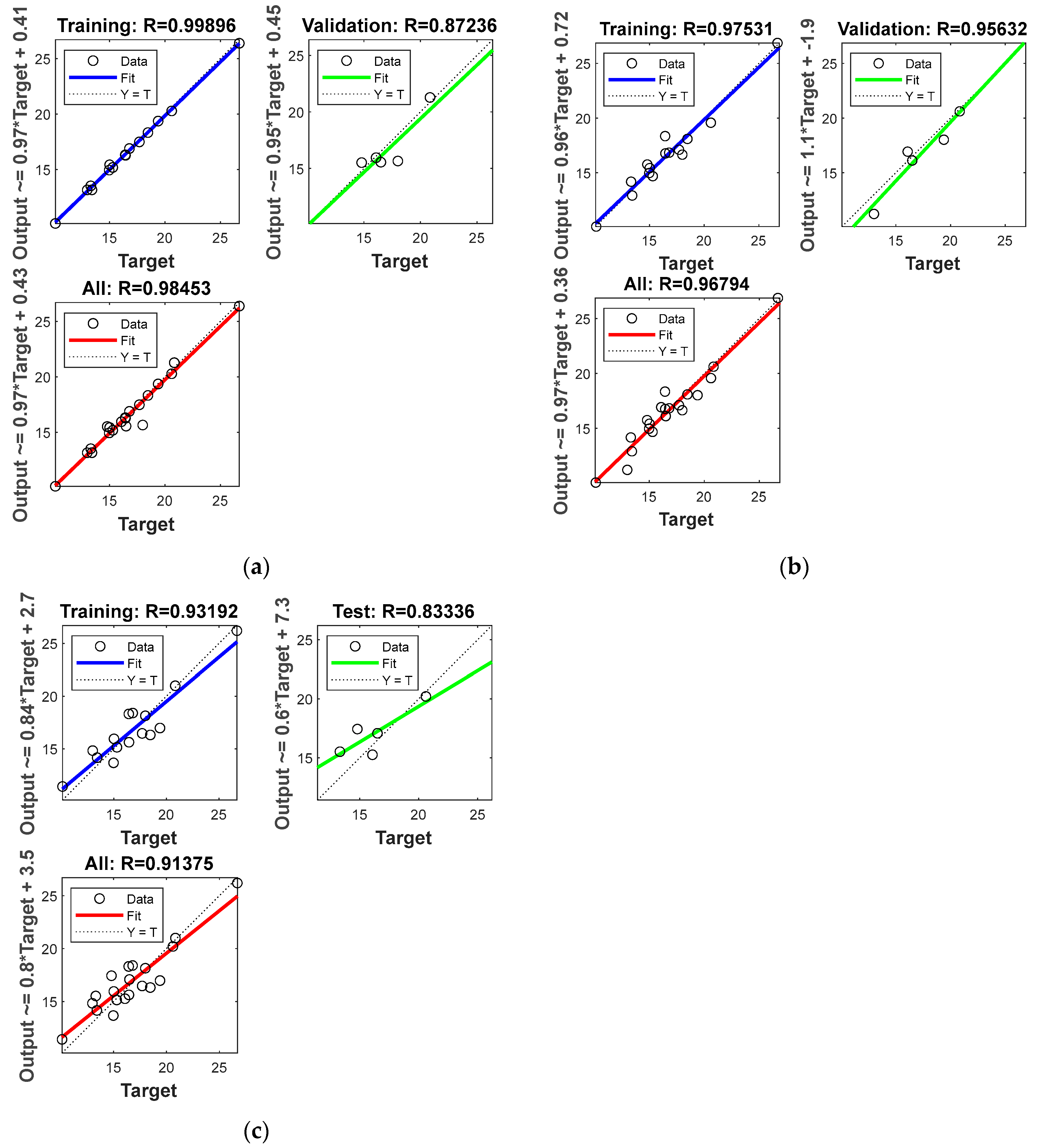
where h(x) = max(0,x). The model consists of six terms based on three predictors: C, H, S, MSE = 0.53114, and R² = 0.95507. Figure 3 and Figure 4 below show the process of finding the best model—the highest value of R² attained for six terms (red color in Figure 3).

3.4. ANN Simulation

Neural networks were analyzed in two variants. In the first one, two variables, C and H, were taken into account in the linear regression analysis; in the second, three predictors, C, H, and S, were obtained in the multivariate spline adaptive regression analysis.

As a result of modeling neural networks with two input neurons, C and H, using the L-M learning algorithm, the best results were obtained with eight neurons in the hidden layer, obtained in 13 iterations. Then, for the network with eight neurons in the hidden layer, the network was trained with the next two learning algorithms: SCG and BR. The results of training these networks are presented in

Table 4. Learning results of neural networks with two input neurons: C and H.

No. of Network	1	2	3
Training algorithm	Levenberg-Marquardt	Scaled Conjugate Gradient	Bayesian Regularization
Epoch	13	27	76
Performance	1.15*10−21	0.573	1.81
Best training performance	1.4215 at epoch 8	1.1868 at epoch 21	1.8125 at apoch 73
Gradient	9.19*10−10	0.993	1.02

.

Quality assessment indicators are given in

Table 5. Results of network quality indicators for networks with two input neurons: C and H.

	Levenberg-Marquardt	Scaled Conjugate Gradient	Bayesian Regularization
R (all data)	0.98453	0.96794	0.91375
MSE	0.3873	0.7789	2.0084
RMSE	0.6223	0.8826	1.4172
MAPE	0.0210	0.0428	0.0768
MAE	0.3577	0.6894	1.1896

. In addition, Figure 5 includes regression plots or training, validation, and all data sets for individual models with learning algorithms: for L-M—Figure 5a, for SCG—Figure 5b, and for BR—Figure 5c. When analyzing the evaluation quality index, the best results were obtained for the network with the L-M learning algorithm.

As a result of modeling neural networks with three input neurons, C, H, and S, using the L-M learning algorithm, the best results were obtained with nine neurons in the hidden layer, obtained in 11 iterations. Similarly, modeling was performed for the networks with the SCG and BR learning algorithms. The results of training these networks are presented in

Table 6. Learning results of neural networks with three input neurons: C, H, and S.

No. of Network	1	2	3
Training algorithm	Levenberg-Marquardt	Scaled Conjugate Gradient	Bayesian Regularization
Epoch	11	26	904
Performance	0.118	0.624	1.25
Best training performance	0.61523 at epoch 5	1.0617 at epoch 20	1.2438 at epoch 159
Gradient	0.296	1.18	0.617

.

Network quality assessment indicators are presented in

Table 7. Results of network quality indicators for a network with three input neurons: C, H, and S.

	Levenberg-Marquardt	Scaled Conjugate Gradient	Bayesian Regularization
R (all data)	0.98827	0.96817	0.90396
MSE	0.2914	0.7672	2.1978
RMSE	0.5398	0.8759	1.4825
MAPE	0.0226	0.0411	0.0694
MAE	0.3794	0.6896	1.0359

, whereas regression graphs for individual models with different learning algorithms are shown in Figure 6. When analyzing the quality indicators, it can be concluded that in this case, similarly to the first variant of the model, the best results were obtained for the network with the L-M learning algorithm.

When comparing the models for each of the variants, the models with the L-M learning algorithm were the best. The first was the model with two inputs (C, H)—Model 1; the second was the model with three inputs (C, H, S)—Model 2. Their comparison is presented in

Table 8. Comparison of model 1 and model 2.

Quality Indicators	Model with 2 Inputs (C, H)	Model with 3 Inputs (C, H, S)
	Model 1	Model 2
R (all data)	0.98453	0.98827
MSE	0.3873	0.2914
RMSE	0.6223	0.5398
MAPE	0.0210	0.0226
MAE	0.3577	0.3794

and in Figure 7.

4. Discussion

Researchers select input parameters for building mathematical models in various ways. Manatura et al. (2023)’s review report on machine learning for biomass showed that the most frequently selected input data are the percentages of C, N, S, O, H, and moisture (M), volatile substances (V), fixed carbon (FC), and ash [39]. In previous studies on models for HHV prediction of biomass, input data are rarely selected using mathematical models. The aim of these studies was to use the multivariate adaptive regression splines approach (MARS) and linear regression (LR) to select input parameters to create a neural network (ANN) model predicting the calorific value (HHV) of biomass produced in Poland. The input data for the conducted analyses included the content of carbon, nitrogen, sulfur, hydrogen, moisture, and volatile matter of wood and field biomass, typically found in Poland. The linear regression results showed that only C and N are significant factors, whereas the other parameters are irrelevant. In MARS, effects are classified as C > H > S, and only these are significant. The R² values for linear regression and MARS are 0.8775 and 0.95507, respectively. These results reveal the better performance of MARS than LR.

Since MARS takes into account three parameters, while LR only covers two parameters in the learning and prediction process, two network models with two variants of input data were created.

In this study, models were compared with different neural network training algorithms: Levenberg-Marquardt (L-M), Bayesian regularization algorithm (BR), and Scaled conjugate gradient algorithm (SCG). Model performance was assessed by taking into account Mean Squared Error (MSE), Root Mean Square Error (RMSE), Mean Absolute Percentage Error (MAPE), Mean Absolute Error (MAE), and correlation coefficients between predicted and actual HHV values. ANN analysis was performed for models with one hidden layer. Adil et al. conducted an ANN model to analyze the concrete mix (ANN structure: 17 inputs and 5 outputs). They revealed that a simple ANN with one or two hidden layers achieved better results than three or more such layers [40]. This outcome implies that ANN analysis with lower hidden layer numbers and more neurons performs better [41,42]. There is no exact method for selecting the number of hidden layers; to find the best predicted results, the selection of the number of hidden layers and neurons is performed iteratively by trial and error. When the number of hidden layers is small, the required training time and cost of the model is lower [43].

In the model with two input variables, the number of neurons in the hidden layer is 8. The results show that the correlation gives a quality of fit of 0.98453 for the L-M algorithm, 0.96794 for the SCG and 0.91375 for the BR. In the second model with three input variables, the number of neurons in the hidden layer is 9, the matching quality was 0.98827 for the L-M algorithm, 0.96817 for the SCG and 0.90396 for the BR. Taking into account the value of R, better values were obtained for the model with three input variables. When analyzing the applied learning algorithms, the highest R and the smallest errors were obtained for the Levenberg-Marquardt algorithm for both created models. As shown in Table 9, this is the algorithm most often used in HHV forecast studies, giving good regression value results. In addition, Jakŝić et al. (2016) compared the qualitative and quantitative analysis of twelve algorithms for training artificial neural networks (ANN) that predict the higher heating value (HHV) of biomass based on proximate analysis (fixed carbon, volatile matter and ash percentage). Of these, the Levenberg-Marquardt algorithm gave the best results in terms of mean squared error calculated on the training set data [44].

Comparison of the error values showed that the ANN model with three input neurons ANN 3-9-1 with the L-M learning algorithm had lower RMSE (0.5398 vs. 0.6223) and lower MSE (0.2924 vs. 0.3873) than the ANN model with two input neurons, with a 2-8-1 structure and an L-M learning algorithm. The research results showed that MARS gave better results in the selection of input variables than LR.

This study focused on the development of an ANN model to predict HHV from biomass. As was mentioned earlier, the relationship between some of the analyzed biomass components and their high HHV calorific value is non-linear; therefore, predicting models based on correlations or linear regression may be insufficient, especially when intending to predict the calorific value of various types of biomass [45]. In the articles that reviewed both linear and non-linear regression approaches to HHV analyses, the models based on non-linearity gave better predictive results [12,46,47]. Comparing the obtained model quality with other models available in the literature that use different HHV prediction methods, the models presented in these studies have the highest correlation coefficients and the best predictive ability. This is evidenced by significantly lower errors than those presented in the literature, as shown in Table 8.

Table 9. Results of ANN as compared to published literature models for biomass.

Model	RMSE	MAE	R2	References
A correlation for calculating HHV from proximate analysis	1.043	0.502	0.359	Parikh et al. (2005) [46]
A correlation for calculating HHV from proximate analysis	1.431	0.679	0.456	Nhuchhen and Salam (2012) [47]
Genetic programming	0.808	0.485	0.934	Ghugare et al. (2014) [45]
Support Vector Machines (SVR) model	3.962	6.172	0.912	Ghugare et al. (2014) [45]
Our model with 2 inputs	0.6223	0.3577	0.968	This study
Our model with 3 inputs	0.5398	0.3794	0.976	This study

Table 9. Results of ANN as compared to published literature models for biomass.

Model	RMSE	MAE	R2	References
A correlation for calculating HHV from proximate analysis	1.043	0.502	0.359	Parikh et al. (2005) [46]
A correlation for calculating HHV from proximate analysis	1.431	0.679	0.456	Nhuchhen and Salam (2012) [47]
Genetic programming	0.808	0.485	0.934	Ghugare et al. (2014) [45]
Support Vector Machines (SVR) model	3.962	6.172	0.912	Ghugare et al. (2014) [45]
Our model with 2 inputs	0.6223	0.3577	0.968	This study
Our model with 3 inputs	0.5398	0.3794	0.976	This study

This paper proposes, develops, and analyzes a new approach using the modeling of artificial neural networks in terms of the selection of input variables for modeling neural networks using MARS and LR analysis. The review of the literature shows that the input data set for ANN modeling appears to be a rather random selection. It should be noted that the amount of input data has a significant impact on the time of creating ANN models. Therefore, it seems that the use of the MARS model for the selection of input variables will allow creating models of artificial neural networks of good quality.

The results obtained in this study are not much different from those found in the literature. A comparison of the proposed ANN model with the existing models is presented in

Table 10. Comparison of the proposed model ANN with the existing models.

Input Variables	Type of ANN	ANN Architecture	R2	Activation Functions	Authors
FC, V, M, A	Levenberg-Marquardt	3-7-1	0.9852	Sigmoid symmetry	[23]
FC, V, M, A	Levenberg-Marquardt	1-23-1-1	0.9591	Hyperbolic tangent sigmoid and linear	[47]
C, H, N, S, O, A, H2O	Radial basis function combined with Levenberg- Marquardt		0.997	Radial basis function	[48]
V, FC, A, M, C, H, N, S, and O	Levenberg- Marquardt	9-10-1	0.985	Tangent sigmoid	[49]
C, H, N, S, O	Levenberg- Marquardt	5-11-1	0.77	Tangent sigmoid	[50]
FC, V, A	Levenberg- Marquardt	3-10-1	0.966	Hyperbolic tangent sigmoid transfer function	[51]
Temperature, Time, FC, V, A, C, O, H	Levenberg- Marquardt	5-10-1	0.8321	Tangent sigmoid	[52]
V, FC, A, M, C, H, N, S, and O	Levenberg- Marquardt	9-10-1	0.909	Tangent sigmoid	[53]
C, H, S	Levenberg-Marquardt	3-9-1	0.976	Hyperbolic tangent sigmoid transfer function	This study
C, H	Levenberg-Marquardt	2-8-1	0.968	Hyperbolic tangent sigmoid transfer function	This study

. The model created shows a high correlation value and low errors. This is additionally confirmed by Figure 7, showing a comparison of the HHV predicted by ANN and the values of models calculated on the basis of real data. On this basis, it can be concluded that the overall compliance of real and simulated data is satisfactory. Such models can be created using different types of biomass, facilitating the selection and widespread use of biomass as a fuel.

Additionally, there is no method for determining the best input variables of a neural network model, MARS can be implemented as a generally accepted method for determining a good subset of input variables when multiple potential variables are considered when deciding inputs for designing a neuron network model.

5. Conclusions

This study developed a machine learning model for predicting the calorific value of selected types of biomass based on input data selected using MARS and linear regression. On the basis of the lowest error values and the regression value, the MARS model was selected as the most accurate for the selection of input data to create a neural network model. The three most important input functions that have a significant impact on HHV prediction were C, H, and S content. It is worth noting that the MARS model presented in this study is better at selecting input data than the LR model.

The best results were obtained for the network with three input neurons and nine neurons in the hidden layer. The resulting model has a high regression value (0.988) and a low root mean square error value (0.3). These studies clearly show that using ANNs is an attractive strategy for estimating the HHV for biomass. The approach presented here can also be usefully extended to accurately estimate the HHV of a wide spectrum of solid, liquid, and gaseous fuels.

References

1. Directive 2009/28/EC of the European Parliament and of the Council of 23 April 2009 on the Promotion of the use of Energy from Renewable Sources and Amending and Subsequently Repealing Directives 2001/77/EC and 2003/30/EC (Text with EEA relevance). Available online: https://eur-lex.europa.eu/legal-content/EN/ALL/?uri=celex%3A32009L0028 (accessed on 5 March 2023).
2. Runge, T.M. Economic and Environmental Impact of Biomass Types for Bioenergy Power Plants. Environmental and Economic Research and Development Program of Wisconsin’s Focus on Energy, Final Report August. 2013. Available online: https://s3.us-east-1.amazonaws.com/focusonenergy/staging/2018-06/1010RungeFinalReportx.pdf (accessed on 5 March 2023).
3. Chen, W.H.; Lin, B.J.; Lin, Y.Y.; Chu, Y.S.; Ubando, A.T.; Show, P.L.; Ong, H.C.; Chang, J.S.; Ho, S.H.; Culaba, A.B.; et al. Progress in biomass torrefaction: Principles, applications and challenges. Prog. Energy Combust. Sci. 2021, 82, 100887. [Google Scholar] [CrossRef]
4. Sivabalan, K.; Hassan, S.; Ya, H.; Pasupuleti, J. A review on the characteristic of biomass and classification of bioenergy through direct combustion and gasification as an alternative power supply. J. Phys. Conf. Ser. 2021, 1831, 012033. [Google Scholar] [CrossRef]
5. McKendry, P. Energy production from biomass (part 1): Overview of biomass. Bioresour. Technol. 2002, 83, 37–46. [Google Scholar] [CrossRef] [PubMed]
6. Xu, L.; Yuan, J. Online identification of the lower heating value of the coal entering the furnace based on the boiler-side whole process models. Fuel 2015, 161, 68–77. [Google Scholar] [CrossRef]
7. Callejón-Ferre, A.J.; Carreño-Sánchez, J.; Suárez-Medina, F.J.; Pérez-Alonso, J.; Velázquez-Martí, B. Prediction models for higher heating value based on the structural analysis of the biomass of plant remains from the greenhouses of Almería (Spain). Fuel 2014, 116, 377–387. [Google Scholar] [CrossRef]
8. Via, B.K.; Adhikari, S.; Taylor, S. Modeling for proximate analysis and heating value of torrefied biomass with vibration spectroscopy. Bioresour. Technol. 2013, 133, 1–8. [Google Scholar] [CrossRef]
9. Khunphakdee, P.; Korkerd, K.; Soanuch, C.; Chalermsinsuwan, B. Data-driven correlations of higher heating value for biomass, waste and their combination based on their elemental compositions. Energy Rep. 2022, 8, 36–42. [Google Scholar] [CrossRef]
10. Hasan, M.; Haseli, Y.; Karadogan, E. Correlations to predict elemental compositions and heating value of torrefied biomass. Energies 2018, 11, 2443. [Google Scholar] [CrossRef]
11. Erol, M.; Haykiri-Acma, H.; Küçükbayrak, S. Calorific value estimation of biomass from their proximate analyses data. Renew. Energy 2010, 35, 170–173. [Google Scholar] [CrossRef]
12. Uzun, H.; Yıldız, Z.; Goldfarb, J.L.; Ceylan, S. Improved prediction of higher heating value of biomass using an artificial neural network model based on proximate analysis. Bioresour. Technol. 2017, 234, 122–130. [Google Scholar] [CrossRef]
13. Nhuchhen, D.R.; Afzal, M.T. HHV predicting correlations for torrefied biomass using proximate and ultimate analyses. Bioengineering 2017, 4, 7. [Google Scholar] [CrossRef] [PubMed]
14. Qian, X.; Lee, S.; Soto, A.M.; Chen, G. Regression model to predict the higher heating value of poultry waste from proximate analysis. Resources 2018, 7, 39. [Google Scholar] [CrossRef]
15. Zagórski, I.; Kulisz, M.; Kłonica, M.; Matuszak, J. Trochoidal milling and neural networks simulation of magnesium alloys. Materials 2019, 12, 70. [Google Scholar] [CrossRef] [PubMed]
16. Kulisz, M.; Kujawska, J. Prediction of municipal waste generation in poland using neural network modeling. Sustainability 2020, 12, 10088. [Google Scholar] [CrossRef]
17. Kulisz, M.; Kujawska, J.; Przysucha, B.; Cel, W. Forecasting water quality index in groundwater using artificial neural network. Energies 2021, 14, 875. [Google Scholar] [CrossRef]
18. Zhou, L.; Song, Y.; Ji, W.; Wei, H. Machine learning for combustion. Energy AI 2022, 7, 100128. [Google Scholar] [CrossRef]
19. Elbeltagi, E.; Wefki, H. Predicting energy consumption for residential buildings using ANN through parametric modeling. Energy Rep. 2021, 7, 2534–2545. [Google Scholar] [CrossRef]
20. Çamur, H.; Al-Ani, A.M.R. Prediction of Oxidation Stability of Biodiesel Derived from Waste and Refined Vegetable Oils by Statistical Approaches. Energies 2022, 15, 407. [Google Scholar] [CrossRef]
21. Patel, S.U.; Jeevan Kumar, B.; Badhe, Y.P.; Sharma, B.K.; Saha, S.; Biswas, S.; Chaudhury, A.; Tambe, S.S.; Kulkarni, B.D. Estimation of gross calorific value of coals using artificial neural networks. Fuel 2007, 86, 334–344. [Google Scholar] [CrossRef]
22. Huang, C.; Han, L.; Liu, X.; Yang, Z. Models Predicting Calorific Value of Straw from the Ash Content. Int. J. Green Energy 2008, 5, 533–539. [Google Scholar] [CrossRef]
23. Estiati, I.; Freire, F.B.; Freire, J.T.; Aguado, R.; Olazar, M. Fitting performance of artificial neural networks and empirical correlations to estimate higher heating values of biomass. Fuel 2016, 180, 377–383. [Google Scholar] [CrossRef]
24. Liao, M.; Yao, Y. Applications of artificial intelligence-based modeling for bioenergy systems: A review. GCB Bioenergy 2021, 13, 774–802. [Google Scholar] [CrossRef]
25. Chou, S.M.; Lee, T.S.; Shao, Y.E.; Chen, I.F. Mining the breast cancer pattern using artificial neural networks and multivariate adaptive regression splines. Expert Syst. Appl. 2004, 27, 133–142. [Google Scholar] [CrossRef]
26. ISO 18134; Solid Biofuels. Determination of Moisture Content. Dryer Method. Part 2: Total Moisture. Simplified Method. International Organization for Standardization: Geneva, Switzerland, 2017.
27. ISO 18122; Solid Biofuels. Determination of Ash Content. International Organization for Standardization: Geneva, Switzerland, 2016.
28. ISO 16948; Solid Biofuels. Determination of Total Carbon, Hydrogen and Nitrogen Content. International Organization for Standardization: Geneva, Switzerland, 2015.
29. ISO 18125; Solid Biofuels. Determination of Calorific Value. International Organization for Standardization: Geneva, Switzerland, 2015.
30. Lalak, J.; Martyniak, D.; Kasprzycka, A.; Żurek, G.; Moroń, W.; Chmielewska, M.; Wiącek, D.; Tys, J. Comparsion of selected parameters of biomass and coal. Int. Agrophys. 2016, 30, 475–482. [Google Scholar] [CrossRef]
31. Friedman, J.H. Multivarite adaptive regression splines. Ann. Stat. 1991, 19, 1–67. [Google Scholar]
32. Milborrow, S. Derived from mda:mars by Trevor Hastie and Rob Tibshirani. Uses Alan Miller’s Fortran utilities with Thomas Lumley’s leaps wrapper. Multivariate Adaptive Regression Splines. Available online: https://cran.r-project.org/web/packages/earth/earth.pdf (accessed on 5 March 2023).
33. Aghelpour, A.; Bagheri-Khalili, Z.; Varshavian, V.; Mohammadi, B.; Marquardt, D. Evaluating Three Supervised Machine Learning Algorithms (LM, BR, and SCG) for Daily Pan Evaporation Estimation in a Semi-Arid Region. Water 2022, 14, 3435. [Google Scholar] [CrossRef]
34. Hagan, M.T.; Menhaj, M. Training feed-forward networks with the Marquardt algorithm. IEEE Trans. Neural Netw. 1994, 5, 989–993. Available online: https://www.mathworks.com/help/deeplearning/ref/trainlm.html (accessed on 12 May 2023). [CrossRef]
35. Burden, F.; Winkler, D. Bayesian regularization of neural networks. Artif. Neural Netw. 2008, 458, 23–42. [Google Scholar]
36. Wali, A.S.; Tyagi, A. Comparative study of advance smart strain approximation method using levenberg-marquardt and bayesian regularization backpropagation algorithm. Mater. Today Proc. 2020, 21, 1380–1395. [Google Scholar] [CrossRef]
37. Møller, M.F. A scaled conjugate gradient algorithm for fast supervised learning. Neural Netw. 1993, 6, 525–533. Available online: https://www.mathworks.com/help/deeplearning/ref/trainscg.html (accessed on 12 May 2023). [CrossRef]
38. Baghirli, O. Comparison of Lavenberg-Marquardt, Scaled Conjugate Gradient and Bayesian Regularization Backpropagation Algorithms for Multistep Ahead Wind Speed Forecasting Using Multilayer Perceptron Feedforward Neural Network. Master’s Thesis, Uppsala University, Uppsala, Sweden, 2015. Available online: https://www.diva-portal.org/smash/record.jsf?pid=diva2%3A828170&dswid=6956 (accessed on 12 May 2023).
39. Manatura, K.; Chalermsinsuwan, B.; Kaewtrakulchai, N.; Kwon, E.E.; Chen, W.H. Machine learning and statistical analysis for biomass torrefaction: A review. Bioresour. Technol. 2023, 369, 128504. [Google Scholar] [CrossRef]
40. Adil, M.; Ullah, R.; Noor, S.; Gohar, N. Effect of number of neurons and layers in an artificial neural network for generalized concrete mix design. Neural Comput. Appl. 2022, 11, 8355–8363. [Google Scholar] [CrossRef]
41. Aniza, R.; Chen, W.H.; Yang, F.C.; Pugazhendh, A.; Singh, Y. Integrating Taguchi method and artificial neural network for predicting and maximizing biofuel production via torrefaction and pyrolysis. Bioresour. Technol. 2022, 343, 126140. [Google Scholar] [CrossRef]
42. Rashid, T.; Taqvi, S.A.A.; Sher, F.; Rubab, S.; Thanabalan, M.; Bilal, M.; ul Islam, B. Enhanced lignin extraction and optimisation from oil palm biomass using neural network modelling. Fuel 2021, 293, 120485. [Google Scholar] [CrossRef]
43. Chen, W.H.; Aniza, R.; Arpia, A.A.; Lo, H.J.; Hoang, A.T.; Goodarzi, V.; Gao, J. A comparative analysis of biomass torrefaction severity index prediction from machine learning. Appl. Energy 2022, 324, 119689. [Google Scholar] [CrossRef]
44. Jakŝić, O.M.; Jakŝić, Z.; Guha, K.; Silva, A.G. Comparing artificial neural network algorithms for prediction of higher heating value for different types of biomass. Soft Comp. 2023, 901, 5933–5950. [Google Scholar] [CrossRef]
45. Ghugare, S.B.; Tiwary, S.; Elangovan, V.; Tambe, S.S. Prediction of Higher heating value of solid biomass fuels using artificial intelligence formalisms. Bioenergy Res. 2014, 7, 681–692. [Google Scholar] [CrossRef]
46. Parikh, J.; Channiwala, S.A.; Ghosal, G.K. A correlation for calculating HHV from proximate analysis of solid fuels. Fuel 2005, 84, 487–494. [Google Scholar] [CrossRef]
47. Nhuchhen, D.R.; Salam, P.A. Estimation of higher heating value of biomass from proximate analysis: A new approach. Fuel 2012, 99, 55–63. [Google Scholar] [CrossRef]
48. Gong, S.; Sasanipour, J.; Shayesteh, M.R.; Eslami, M.; Baghban, M. Radial basis function artificial neural network model to estimate higher heating value of solid wastes. Energy Sources Part A Recover. Util. Environ. Eff. 2017, 39, 1778–1784. [Google Scholar] [CrossRef]
49. Pattanayak, S.; Loha, C.; Hauchhum, L.; Sailo, L. Application of MLP-ANN models for estimating the higher heating value of bamboo biomass. Biomass Convers. Biorefinery 2021, 11, 2499–2508. [Google Scholar] [CrossRef]
50. Brandić, I.; Pezo, L.; Bilandžija, N.; Peter, A.; Šuri´c, J.; Voća, N. Artificial Neural Network as a Tool for Estimation of the Higher Heating Value of Miscanthus Based on Ultimate Analysis. Mathematics 2022, 10, 3732. [Google Scholar] [CrossRef]
51. Veza, I.; Irianto, B.; Panchal, H.; Paristiawan, P.A.; Idri, M.; Fattah, I.M.R.; Purta, N.R.; Silambarasan, R. Improved prediction accuracy of biomass heating value using proximate analysis with various ANN training algorithms. Results Eng. 2022, 16, 100688. [Google Scholar] [CrossRef]
52. Kartal, F.; Özveren, U. Prediction of torrefied biomass properties from raw biomass. Renew. Energ. 2022, 182, 578–591. [Google Scholar] [CrossRef]
53. Xing, J.; Luo, K.; Wang, H.; Gao, Z.; Fan, J. A comprenhesive study on estaming higher heating value of biomass from proximate and ultimate analysis with machine learning approaches. Energy 2019, 188, 116077. [Google Scholar] [CrossRef]
Figure 1. Flowchart of architecture of ANN, LR, and MARS models for HHV prediction.
Energies 16 04162 g001
Figure 2. Response plot graphs a. (a) for linear regression; (b) the predicted response versus true response graphs.
Energies 16 04162 g002
Figure 3. The process of finding the best model.
Energies 16 04162 g003
Figure 4. Response plot graphs for and . (a) MARS (b) the predicted response versus true response graphs.
Energies 16 04162 g004
Figure 5. Regression statistics for individual sets and the total set for: (a) L-M, (b) SCG, and (c) BR for the networks with two input neurons: C and H.
Energies 16 04162 g005
Figure 6. Regression statistics for individual sets and the total set for: (a) L-M, (b) SCG, and (c) BR for the networks with three input neurons: C, H, and S.
Energies 16 04162 g006
Figure 7. Comparison of the real data and the data obtained by model 1 and 2.
Energies 16 04162 g007