Article

Systematic Method for Developing Reference Driving Cycles Appropriate to Electric L-Category Vehicles

1
Institute for Transport Studies, University of Leeds, Leeds LS2 9JT, UK
2
Centre for Innovation, Technology and Policy Research (IN+), Associação para o Desenvolvimento do Instituto Superior Técnico, Universidade de Lisboa, Avenida Rovisco Pais, 1049-001 Lisboa, Portugal
3
Mechanical Engineering Department, Instituto Superior de Engenharia de Lisboa (ISEL), Rua Conselheiro Emídio Navarro 1, 1959-007 Lisboa, Portugal
4
School of Mechanical Engineering, Beijing Institute of Technology, Beijing 100081, China
*
Author to whom correspondence should be addressed.
Energies 2022, 15(9), 3466; https://doi.org/10.3390/en15093466
Submission received: 4 February 2022 / Revised: 26 April 2022 / Accepted: 27 April 2022 / Published: 9 May 2022

Abstract

:
Increasingly, demanding environmental standards reflect the need for improved energy efficiency and reduced externalities in the transportation sector. Reference driving cycles provide standard speed profiles against which future developments and innovations may be tested. In the paper, we develop such profiles for a class of electric L-category vehicles, which are anticipated to play an increasing future role in urban areas. While such driving cycles exist for regular L-category vehicles, these may not be suitable in the case of electric vehicles, due to their power output limitations. We present a methodology for deriving these new driving cycles, developed from empirically deduced power relationships, before demonstrating their application under different assumptions on the terrain and vehicle characteristics. The applications demonstrate the feasibility of the method in developing appropriate driving patterns for alternative real-world contexts. On flat terrain, the adjustments made to cope with the power limitations of L-EV do not introduce significant differences in energy consumption, suggesting that the certification does not require extensive modification. However, when considering road slope, differences of up to 5% in energy use and up to 10% in regenerated energy were observed, showing the importance of the developed method for assessing vehicle performance in real-world driving.

1. Introduction

Due to the severe problems, such as global warming and harm to human health, caused by internal combustion engine-powered vehicles, electric vehicles have been attracting increasing attention [1,2,3]. They enable higher energy efficiency without exhaust emissions, and the use of electricity incorporating higher percentages of renewable energy resources plays a significant role in enabling improved life-cycle impacts compared to conventional technologies [4,5]. The inventory of electric vehicles continues to increase significantly, with over 7 million vehicles worldwide in 2019 [6]. Furthermore, their purchase cost barriers are expected to be alleviated by the anticipated evolution in battery technology [6,7]. Consequently, electric vehicles are expected to be the main mode of personal passenger transport in the future.
Furthermore, urban mobility brings additional challenges in terms of use of space, parking requirements, and the associated drive cycle, bringing opportunities for small electric vehicles, which have the particular benefits of small size, low cost, and low energy consumption for short-distance travelling [8]. While many different names and classifications exist for such vehicles around the world, we refer to them as L-category electric vehicles, following the terminology used in Europe and based on the class of vehicles that is specifically used in our case study [9]. This class of vehicles is framed within the L7 category for quadricycles, whose unladen mass is not more than 400 kg (not including the mass of batteries in the case of electric vehicles) and whose maximum net engine power does not exceed 15 kW [10]. These small vehicles are generally within the M1 category according to the UNECE global technical regulations [11,12]. However, this classification changes over the geographical area. In India, quadricycles must comply with the maximum permissible kerb weight of 450 kg in case of a passenger vehicle, up to 15 kW maximum power and a maximum speed of 70 km/h [13]. In Korea, these vehicles are included within the concept of micro-mobility, defining maximum allowable dimensions (length up to 3.6 m, width up to 1.5 m, height up to 2.0 m), as well as a maximum power of 15 kW and a maximum mass of 600 kg [14]. In the U.S., quadricycles fall within the class of Low-Speed Vehicles, whose speed attainable in 1.6 km (1 mile) is more than 32 km/h and lower than 40 km/h, also limiting Gross Vehicle Weight Rating up to 1134 kg due to safety purposes [15,16]. Elsewhere, other regional rules can apply, however it can be stated that, generally, quadricycles represent a mobility opportunity due to their small size, low power and weight, energy efficiency, and suitability for all types of drivers.
With their more efficient use of space due to their small size, the increased use of L-category electric vehicles has the potential to reshape urban mobility. One of the main applications is as the first-mile or last-mile access mode for a longer journey [17]. Especially under epidemic situations, L-category electric vehicles could be a good option to decrease infection spread by reducing public transport use for those who cannot afford conventional electric vehicles. The relatively low purchase and operating costs of such vehicles also provide them with the potential to better address concerns over social inequalities concerning energy poverty [18].
Thus, although the current market for L-category vehicles is relatively small (Santucci et al., 2016, estimated around 10,000 had been sold within EU countries by that date), their great potential in benefiting our lives suggests they deserve greater attention. Indeed, as the market analysis model forecasts have shown [19], their sales volume is likely to continue to grow for the foreseeable future. One of the first examples of these L-category electric vehicles was the Renault Twizy [20], launched in 2012, with a more recent (2020) example the Citröen Ami [21], suggesting that this type of vehicle is seen as an opportunity by major vehicle manufacturers. According to the plan approved by the European Commission for achieving clean urban transport, the goal is that “by 2050 nearly all cars, vans, buses as well as new heavy-duty vehicles will be zero-emission” [22], while at the same time encouraging the use of smaller, lighter and more specialized road passenger vehicles [8], namely focused on micro-mobility.
The popularization of L-category electric vehicles will most probably be fostered by the increasingly accepted concept of micro-mobility and mobility as a service, but its adoption relies on the existence of a correlated test procedure necessary to ensure their production consistency and to meet the requirements of consumers, namely regarding energy consumption. For M-category (light-duty vehicles, passenger cars and vans, carrying passengers) electric vehicles, certification driving cycles and procedures are well established. However, their representativeness can be discussed, since differences have been found between energy use within certification cycles and real-world conditions [23,24,25,26]. Consequently, even for M-category vehicles, the pursuit of representative drive cycles for alternative vehicle technologies based on real-world use has also started to be explored. For example, Zhang et al. developed tailored driving cycles for electric vehicles based on a sample of 40 electric taxis, by developing a Markov Monte Carlo method considering the driving features of different roads [27]. Defining a driving cycle for a test procedure is the main basis for assessing vehicle performance [28,29], particularly for electric vehicles where regeneration plays an important role in the gross energy consumption.
A detailed test procedure is available for a different type of L-category vehicle to that considered in the present paper, namely those powered by an internal combustion engine [30]. However, since L-category vehicles have power and weight limits (without a battery), additional mass associated with energy storage could limit the power-to-weight ratio, possibly leading to differences in their driving capabilities, as has been observed from comparisons of conventional L-category vehicles and electric ones [31,32]. Problems may therefore arise if the driving cycle of a conventional L-category vehicle is applied to the performance assessment of electric modes, such as the electric ones being unable to follow the driving cycle due to their small-rated power-to-weight output.
Due to the short running distance of L-category electric vehicles, they are more suitable for urban utilization. In real-world driving, traffic conditions are much more complex than the ones considered in driving cycles [33]. One study quantified that traffic conditions and driving behaviour may increase energy consumption by up to 40% and 16%, respectively, compared to the worst performance condition [34]. Regarding road grade, ascending roads (with 3% grade) increased energy consumption by 50% while descending roads (−3% grade) decreased energy consumption by 80%, due to the presence of regenerative braking systems. These facts may lead to more difficulty for L-category electric vehicles in real driving, such as on hilly terrain where acceleration is limited due to their power output.
Additionally, in urban driving, vehicles are periodically under stop-and-go situations [35] (e.g., resulting from many traffic lights), which will cause much energy loss if the energy regeneration technology is missing [25]. With regards to the L-category electric vehicles on the market, most of them do not include energy recovery devices leading to lower energy efficiency performance. Energy loss will be significant if the vehicle is travelling downhill where brake actions are necessary to ensure safety and to be within the speed limit. Furthermore, a better understanding of real-world performance in specific routes, acknowledging the influence of road grade and traffic, may also contribute to better route optimization and charging optimization systems [36,37].
Therefore, it has been shown that M-category vehicles have well-established certification procedures but do not incorporate real driving energy consumption in a generalized way. For L-category vehicles, the certification procedures are mostly suited to conventional propulsion technologies and do not consider real driving energy use, which gains importance due to their limited power-to-weight ratio or the possibility of regeneration. Taking into consideration the emergence of L-category electric vehicles in an urban context and their power-to-weight limitations, this paper proposes an innovative approach for evaluating current certification drive cycles available for this vehicle class and compares them with real-world driving cycles. The impacts of regenerative capabilities and road grade on the L-category vehicles’ energy performance are also assessed, paving the way for improved future energy characterization of a growing vehicle market.
The structure of the paper is as follows. Firstly, in Section 2 we describe the previously-reported experimental data that we will re-purpose for the study, and begin to explain the specific motivation for our work. In Section 3 we present the details of a generic methodology for modifying a given reference speed profile to apply to a vehicle with generally lower power capabilities. This methodology is applied in Section 4 to a particular case of electric L-category vehicles, where the sensitivity of the method is explored in tests on fictitious gradient profiles. In Section 5, it is applied to a realistic case of road profiles from the city of Lisbon. Finally, conclusions and directions for further research are described in Section 6.

2. Experimental Data Description and Motivation

2.1. Empirical Evidence of L-Category Electric Vehicle Characteristics

The method to be described requires knowledge of the characteristics of the electric vehicle under study, in particular the relationship between velocity, acceleration, and vehicle specific power [38]. Here, we draw on the relationships derived in a real-world study of electric quadricycles [23]. The general specifications of the quadricycles used as a basis for this work, are presented in Table 1 and can be found in more detail in reference [23].
Let f ( v , a ; θ ( x ) ) denote the function whose output is the instantaneous Vehicle Specific Power (VSP) (in W/kg) corresponding to a velocity of v (m/s) and acceleration a (m/s2), given a parameter vector θ ( . ) that defines the relevant properties of the vehicle type under consideration and the local road surface at a given location x . Alves et al. [23] demonstrate how a simplified form of this relationship may be derived for f ( . ) , of the form:
f ( v , a ; θ ( x ) ) = ( 1.1 a + 9.81 θ 1 ( x ) + θ 2 ) v + θ 3 v 3
where θ 1 ( x ) ,   θ 2 and θ 3 are respectively the grade (in m/m) at location x , coefficient of rolling resistance (in N/kg) and coefficient of aerodynamic drag (in Ns2/m2kg).
In addition, Alves et al. posited a relationship for the function e ( p ; β ) , denoting the instantaneous Energy Consumption Rate (ECR, in Wh/s) corresponding to an instantaneous VSP of p (W/kg), given parameter vector β (which differs by vehicle type). They supposed e ( . ) to be a continuous, piecewise-linear function of the form:
e ( p ; β ) = { β 1 p + β 2 p < 3 β 3 p + β 4 3 p < 0 β 5 p + β 6 0 p < 3 β 7 p + β 8 p 3 .
Note that this energy relationship explicitly models negative instantaneous events arising from negative VSP, arising from the regenerative braking capability of the vehicles considered. While Equation (1) is the main element required to apply our method, Equation (2) will prove useful in our sensitivity analyses, to judge the consequences of different assumptions on overall energy consumption.
Relationship (1) will be used later in the paper as the basis for developing relevant speed profiles, and relationship (2) will be used to assess the energy impacts of alternative speed profiles. In fact our methodology is rather generic, in that if desired alternative power and energy relationships may be implemented using the same techniques. Before continuing we provide some reflection on our choice of (1) and (2) as the basis of our numerical demonstrations, and discuss how alternative approaches may be implemented:
  • In our analysis we suppose a single value for the coefficient of rolling resistance, θ 2 in (1). The methodology used is based on already published work, which follows established methods, namely the Vehicle Specific Power (VSP) methodology [23,38,39,40,41,42,43]. The simplicity and accuracy of the VSP which is followed here, with coefficients provided from already published work [23] is one of the main strengths of this method. In reality θ 2 may vary over time depending, for example, on whether road surface conditions are wet or dry. The method we subsequently present is sensitive to the value of θ 2 , and so if different values of θ 2 were known relevant to the prevailing weather conditions, then different speed profiles may be deduced relevant to the situation under study. In addition our method allows sensitivity testing of the impact of deriving the speed profile with (say) a wet weather θ 2 when the weather is in fact dry; this would follow the same process as we follow in Section 4.2 for testing a different parameter, when instead we test the effect of using a profile derived for flat terrain on a hilly terrain. A simple extension of this would be to represent the impact of modeller uncertainty by assuming a distribution of true θ 2 values, randomly sampling from this distribution, and then evaluating the performance of a speed profile derived from some given θ 2 = θ ^ 2 .
  • Our methodology and derived speed profiles do not depend on (2); however, this equation is used to evaluate the energy impacts of the speed profiles, and so this evaluation is sensitive to the assumed value of the β parameter. The detailed process for estimating the values in β we shall assume is described in the source reference [23], based on 1 Hz data in order to represent a large range of driving conditions. Again, this is based on the scientifically accepted VSP methodology, which uses representative coefficients obtained from the characteristics of the vehicles studied. For instance, rolling resistance is based on the tyre properties, and the aerodynamic coefficient is based on the aerodynamic resistance coefficient and frontal area. Since a modal analysis is made, the numerical value calculated for VSP based on the coefficients is the same as that collected under real-world conditions. Consequently, a VSP value calculated for a speed cycle (based only on speed, acceleration and topography) corresponds to a certain amount of energy used (monitored, measured) or harvested under real-world conditions with a similar VSP value. These variables have physical meaning and are adapted for bicycles, motorcycles, quadricycles, light-duty and heavy-duty vehicles. However, they do not interfere deeply in the implementation of VSP, since measured energy consumption values are associated to driving conditions, allowing the estimation of energy used on a driving cycle without effectively running that driving cycle with a particular vehicle. If it is desired to test the sensitivity with respect to β then we note that this is even more easily achieved than testing the impact of alternative power assumptions, since the derived speed profiles do not depend on the relationship between energy and VSP, only on the relationship between VSP and speed, acceleration and the features of the vehicle and physical environment.
  • The remarks in the two points above are examples of a wider issue, whereby it could be argued that all of the parameters in (1) and (2) have uncertainty associated with them, either because they vary in the real-world (within or between vehicles, or due to environmental conditions), or because of modeller uncertainty. Our methodology is readily applied to study such impacts by the kinds of methods already described in the two points above. In our later analysis (Section 4) we study one such example of real variation by exploring the impact of different types of vehicle, as well as one such example of modeller uncertainty in terms of road topography. Such an analysis could be repeated with a range of randomly sampled values, to represent either true variation or modeller uncertainty, and could be repeated for the whole range of parameters β ,   θ 1 ( x ) ,   θ 2 and θ 3 . On the other hand, when considering VSP in particular, the use of fixed values for the parameters of the VSP relationship has been widely studied, with calibration results leading to errors below 5% for electric vehicles [23]. Consequently, our own subsequent analysis based on fixed parameter values is unlikely to lead to significant error.
  • Alternative non-linear forms to the ECR relationship (2) may also be considered; the piecewise-linear form was motivated in the original source paper by considering the ‘breakpoints’ at which different energy consumption states arise. By combining the above equations for VSP and ECR, the basic assumption is that the instantaneous energy consumption at time t is related to the vehicle velocity and acceleration at the same time t. Our ultimate objective will be to adapt a reference speed profile (developed for a different vehicle technology) to conform to the physical constraints of a new technology, as captured in the above equations. Alternative methods exist for more sophisticated analysis of such temporal profiles, such as wavelet transformations, and these would be particularly suited to future research focused on forecasting [44] or feature extraction [45].
In their empirical study [23], Alves et al. estimated the parameters of Equation (1) for the quadricycle class to be:
θ 2 = 0.159           θ 3 = 0.984 × 10 3
and estimated the parameters of Equation (2) to differ by the specific type of quadricycle monitored, as in Table 2.
A final important estimated element was the maximum VSP. Rather than a physical limit of the battery/vehicle, the estimated value was more of a ‘behavioural limit’, namely a value below which 99% of the measured VSPs fell in the real-world driving experiments. These 99th percentile VSPs, which will be used as the maximum VSPs in the methodology presented below, were estimated (when rounded to the nearest integer) as 9, 9, and 12 for vehicle types 1, 2, and 3 respectively.

2.2. Reference Driving Cycles for Conventional L-Category Vehicles

Independently from the work described in Section 2.1, the World Harmonised Motorcycle Test Cycle (WMTC) is a system of driving cycles, specifically for measuring environmental emissions [46], and which are intended to represent real-world driving conditions. These are used as part of the detailed technical requirements and test procedures for the approval of L-category vehicles in the EU. While not developed with the requirements of electric L-category vehicles in mind, they nevertheless represent an important standard, and specifically, the two cycles for urban driving conditions (where electric L-category vehicles will likely operate) represent important reference points for any work designed at developing new driving cycles. These two cycles will be referred to subsequently in this paper as (WMTC) Reference Cycles 1 and 2. The speed and acceleration profiles are displayed later in this report, as comparators as we seek to adjust them.

2.3. Issues with Adopting Reference Cycles for Electric L-Category Vehicles

As motivation for our later work to be presented, we illustrate the problem of directly combining the evidence and relationships described in Section 2.1 with the reference cycles in Section 2.2. In Figure 1 WMTC Reference Cycle 2 is illustrated, and in Figure 2, the implied time-profile of vehicle specific power, if an electric quadricycle (with the characteristics defined in Section 2.1) were to follow the speed/acceleration profile in Figure 1 over a flat terrain.
Note that, as intended with the power model developed in [23], both positive and negative VSP values arise, the negative values corresponding to intervals of regenerative braking (corresponding to 15.65% of time in WMTC Reference Cycle 2), where the vehicle’s kinetic energy is converted back to electrical energy. On the other hand, peaks of VSP, corresponding to acceleration events in the reference cycle, give rise to VSP values that exceed the maximum of 9 estimated for vehicle type 1 or type 2, with the VSP exceeding the maximum for 5.16% of the time duration of the driving cycle. In this respect, the reference cycles are thus not realistic for the performance or driving characteristics of electric L-category vehicles.
Typically, reference cycles are developed assuming a flat terrain and we are not aware of corresponding cycles taking gradient into account. As an experiment, though, we repeat the same test as above, but now instead of assuming a hilly terrain, using the gradient function described later (see Section 4) which is uphill for the first half of the road section and downhill for the second, but with the start and endpoints on the same elevation (i.e., zero net gain in elevation over the whole profile).
In Figure 3, we can observe more pronounced peaks of the VSP in the first half of the cycle (on the uphill section of the route), and a lesser violation of the maximum on the second (downhill) half. This balances out to in fact a lesser overall time (4.83%) exceeding the VSP bound than the flat-terrain case, and a greater time (17.65%) in negative power states. More relevant than these summary measures is, however, the fact that when it does exceed the bound it exceeds it by more, making it even more physically infeasible.
From these initial experiments, we can highlight some key, distinctive features:
-
it is important that the positive impact on energy consumption of regenerative braking, as uniquely present in electric vehicles, can be captured in any reference profiles;
-
the speed/acceleration profiles developed for regular L-category vehicles may not be attainable by electric L-category vehicles, particular when speed/acceleration is high;
-
any adjusted driving cycle for electric L-category vehicles should consider the sensitivity to the gradient of the terrain on which they are driven.
Addressing these features will serve as the main motivation for the present paper.

3. Methodology for Creating Adjusted Speed Profiles

3.1. Goals of Methodology

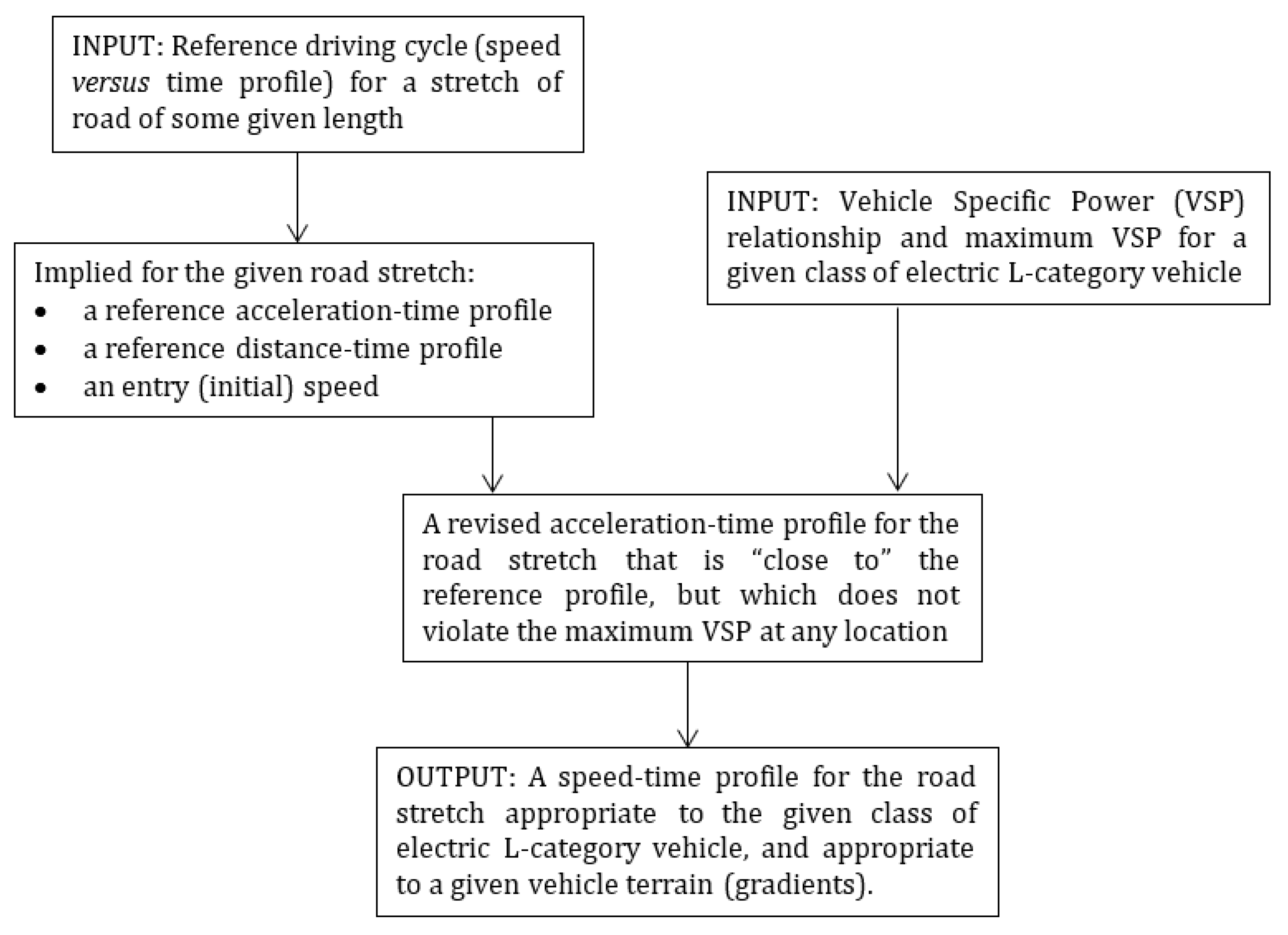
An overview of the methodology to be applied is presented in Figure 4. It assumes as inputs (a) a given reference speed profile, and (b) a relationship between VSP and (speed, acceleration, gradient) for a given vehicle type, along with a maximum VSP. Equivalently to working with the reference speed profile in (a) we may derive from it a reference acceleration profile and initial speed at the entry to the road stretch; in addition, a reference distance-time profile may be deduced. The goal of the adjustment process is to derive an adjusted acceleration profile that does not violate the given maximum VSP.
At first sight, since high VSP values are typically associated with high acceleration events, this might seem to be a quite trivial task of simply bounding the acceleration profile at some given maximum. However, on closer inspection, there are several complications to this process, and it is these considerations that motivate our method (to be subsequently described):
  • From Equation (1), it can be seen that high VSP values arise from a combination of speed, acceleration, and gradient; it is not simply that there is a maximum acceleration, regardless of speed or gradient.
  • Given speed and gradient, Equation (1) is easily rearranged to make acceleration a function of VSP, and a maximum acceleration is then deduced given the maximum VSP. If done in continuous time, then this would indeed impose the maximum VSP constraint. However, the reference profiles are specified at a given time discretization. If we compute the maximum acceleration, given the speed at the start of a time increment, so as to be bounded by the maximum VSP, then by the end of the time increment the vehicle (since accelerating) will be going faster, and so may violate the maximum VSP by the end of the time increment.
  • In general, the adjustment process will result in lower acceleration and lower speeds. As a result, downstream from any adjustment made during an acceleration event, we may have a deceleration event with physically impossible consequences, i.e., a negative speed.
  • As noted, the adjustment process will generally result in lower speeds. The reference speed profiles are intended to represent travel over a road stretch of a given length, but are specified by a speed profile over a given time period. If the adjusted speed profile is applied for the same time period, then it will not represent the same length of road, since by the end of the time period, the vehicle (travelling at lower speeds) will not have reached the end of the road stretch. Thus, in tandem with adjusting speeds, a logical method is needed for extending the time period over which the driving cycle applies, so that it applies to the same road length.
In brief, points 1 and 2 are addressed by a numerical search (Newton) method at each time increment, which deduces the maximum acceleration possible at the current location, given the current gradient, and given the consequential effect of that acceleration on the speed at the end of the time increment. Point 3 is handled by bounding acceleration so that the consequential speed at the end of the increment is at least zero. Point 4 is dealt with essentially by assuming that speed reduction will mean that vehicles will tend to cruise for longer; it is as if there is a vehicle following the unadjusted speed profile, with which our adjusted vehicle tries wherever possible to ‘catch up’ in terms of the distance traversed. Taken together, these three adjustment processes are thus concerned with acceleration, deceleration, and cruising respectively. The three processes are first described in more detail in Section 3.2, Section 3.3, and Section 3.4 respectively, before presenting the overall algorithm in Section 3.5.

3.2. Acceleration Steps: Bounding of Acceleration

Consider a particular increment of time of length Δ seconds, and suppose that we are given the speed u m/s and location from some origin x metres of a vehicle at the start of the time increment. The aim will be to determine the constant acceleration a m/s2 during that increment, and thereby the resulting speed v m/s at the end of the time increment. Clearly by standard equations of motion:
v = u + a Δ
and the location y of the vehicle at the end of the time increment is given by:
y = x + u Δ + a Δ 2 2 .
Then, according to Equation (1), we may associate a VSP with any (location, speed, acceleration) triple ( y , v , a ) . Since we are imagining time increments in the order of seconds, then the road gradient will hardly change between location y and x , so we approximate θ 1 ( y ) θ 1 ( x ) for some simplification. Then the VSP at the end of the time increment f ( v , a ; θ ( x ) ) is obtained by combining Equations (1), (4) and (5) to give:
f ( u + a Δ ,   a ; θ ( x ) ) = ( 1.1 a + 9.81 θ 1 ( x ) + θ 2 ) ( u + a Δ ) + θ 3 ( u + a Δ ) 3 .
Thus, given the (location, speed) ( x , u ) at the start of the time increment, the VSP at the end of the time increment may be thought of as a function only of the acceleration a , parameterized by ( x , u ) :
ϕ ( a ; x , u ) = ( 1.1 a + 9.81 θ 1 ( x ) + θ 2 ) ( u + a Δ ) + θ 3   ( u + a Δ ) 3 .
By inspection, ϕ is monotonically increasing in a , and so its inverse function exists. Let ψ ( p ; x , u ) denote this inverse function for a VSP p given ( x , u ) , i.e., such that:   a = ψ ( ϕ ( a ; x , u ) ; x , u )   a .
Now let p max denote the assumed maximum VSP of a vehicle under consideration. We may then, by the reasoning above, calculate a maximum acceleration a max corresponding to the maximum VSP p max according to a max = ψ ( p max ; x , u ) . Note that this maximum acceleration is not constant, depending through ψ on the current speed u and local conditions in terms of gradient through x ; this is implicitly handled through the method described (so we could write a max ( x , u ) to denote this dependence).
Since the inverse function is not available in analytic form, the procedure is to instead numerically estimate the acceleration a that satisfies ϕ ( a ; x , u ) = p max or equivalently ϕ ( a ; x , u ) p max = 0 . This is done via a Newton scheme whereby the ( k + 1 ) th iteration is given by:
a ( k + 1 ) = a ( k ) ϕ ( a ( k ) ; x , u ) p max ϕ ( a ( k ) ; x , u )
where ϕ ( a ; x , u ) is given by (7) and:
ϕ ( a ; x , u ) = 1.1 ( u + a Δ ) + Δ ( 1.1 a + 9.81 θ 1 ( x ) + θ 2 ) + 3 θ 3 Δ ( u + a Δ ) 2 .

3.3. Deceleration Steps: Bounding of Deceleration

The adjustments described in Section 3.2 will in general decrease (or leave unaltered) accelerations and speeds, relative to the reference values. Suppose that we are considering a particular time-step, and that in a previous time-step the bounding of acceleration has indeed resulted in a speed reduction relative to the reference speed. Thus, even before we consider what might happen in the current time-step, the vehicle may be travelling at a lower initial speed than the reference speed at the start of the time-step. Now consider the current reference acceleration; if it is negative, then there is no guarantee that such a deceleration will be feasible from the initial speed, as it may result in a negative speed by the end of the time increment. In practice, this is quite a rare occurrence, but it can occur and lead to physically impossible profiles. Therefore, a simple adjustment is made for deceleration events, namely that given any time-period (length Δ ) and an initial speed at the start of that time period u , then the acceleration a is bounded below so as the speed at the end of the time-interval v is no less than zero:
v = u + a Δ 0
implying:
a u Δ    

3.4. Cruising Steps: “Catching Up” Distance

The third and final type of step is the cruising one. This arises as we aim to specify a speed profile for a road segment of a given length. The main speed adjustment steps (as described in Section 3.2) will mean that in the adjusted profile the speeds will generally be lower than in the reference profile. If we specify the adjusted profile for only the same number of time steps as the reference profile, a vehicle following that trajectory will then clearly only traverse part of the road segment by the end of the time period. For a slower vehicle to traverse the same length as a vehicle following the reference profile, it must travel for longer in time. The question is: what logic might we use to add additional time periods?
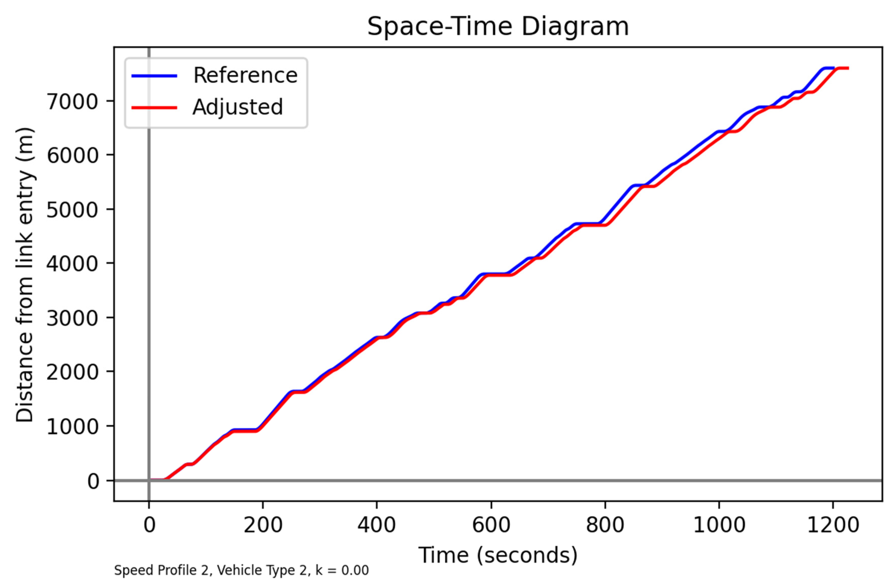
The approach is based on the premise that the variations in speed/acceleration in the reference profile are associated with spatial (as opposed to temporal) locations on the route, e.g., intersections, locations where queuing occurs. Therefore, the adjusted speed profile should, where possible, aim to track the spatial variations in the reference speed profile. It can be imagined that a vehicle following the (slower) adjusted profile is trying to ‘catch up’ the distance travelled by a vehicle following the reference profile, and so each time it falls behind it will cruise at the current speed for several time steps. The effect of this, as seen in 
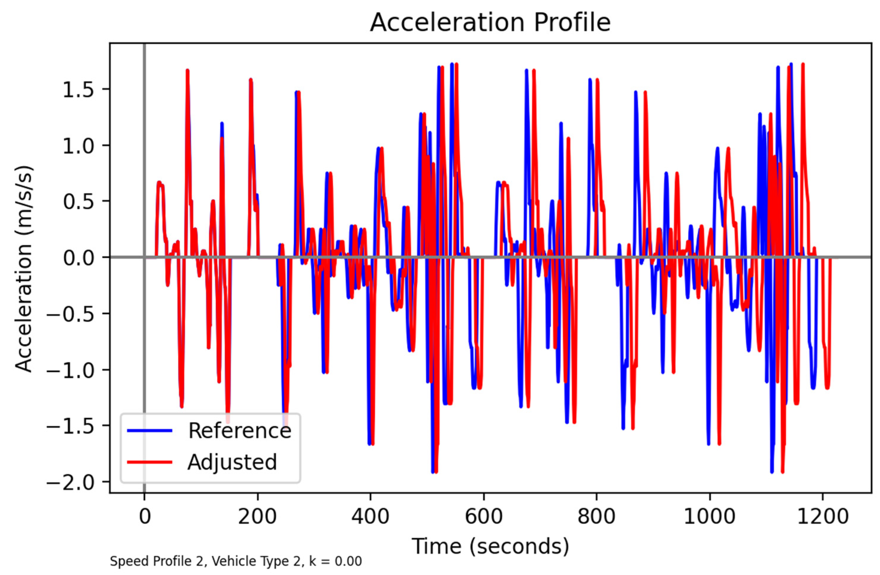
Section 4, is that the peaks of the adjusted profile both lag behind those of the reference profile in time, as well as being somewhat extended; this seems logical behaviorally, that someone travelling at a slower speed than another vehicle will just maintain that slower speed for longer to reach the same point.
Suppose then, having applied a step from Section 3.2 or Section 3.3 as appropriate, to a given reference time increment, the total distance travelled on the adjusted profile so far is x metres, and the distance travelled using the reference speeds by the end of this reference time interval is x REF . Then the cumulative lost distance relative to the reference profile is D = x x REF . Suppose that when applying the methods of Section 3.2 or Section 3.3 an adjusted speed of v ˜ m/s was determined for the end of the last time increment. If v ˜ = 0 then skip this step; so let us assume now that v ˜ > 0 . Firstly, we determine whether the vehicle is in a ‘cruising mode’, and if it has reached some desired speed. This is indicated either by the reference acceleration for the previous period a REF being equal to zero, or by the fact that the reference acceleration is about to “pass through” zero if it were not for discretization. This latter state is indicated by a positive reference acceleration a REF   for the previous period and a negative reference acceleration a REF + for the following period.
Hence overall our test is:
v ˜ > 0   and   { a REF = 0   or   { a REF > 0   and   a REF + < 0 } }  
We now check whether additional time increments can be inserted with the vehicle cruising at a speed of v ˜ , without the distance for these increments exceeding D . Due to the discretization, we are unlikely to be able to catch up all the distance in D (though that is the goal), so instead, we insert as many time increments as possible in order to travel as close as possible to D metres. Since by cruising at a speed of v ˜ m/s we will travel Δ v ˜ metres in one time increment of Δ seconds, the number of time increments we will be able to insert is:
number   n   of   cruising   time   intervals = [ D Δ v ˜ ]
where for any real number x the notation [ x ] denotes the largest integer x . These time increments are then inserted, before moving on to consider the next time increment from the reference speed profile.
Having applied this process to the full time period of the reference speed profile, it is likely that there will be a small amount of cumulative lost distance remaining at the end. This is accounted for by rewinding to the last time at which cruising increments were inserted, and inserting additional increments at that time to account for as much of the remaining cumulative lost distance as is possible within the error of discretization.

3.5. Overall Solution Process

The solution process makes use of three methods corresponding to the techniques described in Section 3.2, Section 3.3 and Section 3.4. A method in this sense is a computational process with given inputs and outputs as follows:
( a , ˜ v ˜ ) = BoundAcceleration   ( x , u , Δ , p max , a REF )
( a , ˜ v ˜ ) = BoundDeceleration   ( u , Δ , a REF )
n = CalculateCruisingTime   ( v ˜ , D , Δ ) .
The method BoundAcceleration , applied only when a REF > 0 , first estimates an upper bound on acceleration over a time interval of length Δ seconds given an initial speed of u m/s and given a bound on vehicle specific power of p max W/kg. The acceleration bound will vary with both speed u and location x (the latter dependence due to variations in gradient). The upper bound is estimated by the iterative process (8) based on (7) and (9), with the converged solution denoted a max (m/s2). The method then provides as output the bounded acceleration a ˜ (in relation to the input reference/default acceleration a REF ) and the corresponding speed v ˜ according to:
a ˜ = min ( a REF , a max )                       v ˜ = u + a ˜ Δ   .
The method BoundDeceleration , applied only when a REF < 0 , bounds acceleration from below to avoid physically impossible (negative) speed on exit from the time increment. It provides as output the bounded acceleration a ˜ (in relation to a REF ) and corresponding speed v ˜ according to:
a ˜ = max ( a REF , u Δ )                       v ˜ = u + a ˜ Δ .
The method CalculateCruisingTime is applied after either of the two methods above, and only when three conditions are all met: (i) the adjusted speed v ˜ > 0 , (ii) the reference acceleration is indicative of cruising ( a REF = 0 or { a REF > 0 and a REF + < 0 }), and (iii) the cumulative lost distance D > 0 . It provides as output the maximum number n of time intervals of length Δ seconds at which a vehicle may cruise at v ˜ m/s in order to recover the most lost distance, according to (13). An implementation issue to note is that since a R E F is stored as a real number, the practical test of “zero acceleration” applied is | a R E F | < ϵ for some small ϵ > 0 .
With these three methods as the building blocks, it is then possible to describe the overall adjustment process. Suppose that a vehicle is moving in time and space along a stretch of road of given length L metres, and that time is discretized into increments of length Δ seconds. Let { v 0 REF , v 1 REF , , v m REF } denote the speeds over time increments in a given reference driving cycle, with v i REF m/s the reference speed at the end of the i th time increment (i.e., so at continuous time i Δ ). Assuming uniform acceleration within a time increment (between the exit speed of the last time increment and the exit speed of the present one), Equation (4) may be applied to additionally infer a reference acceleration profile { a 1 REF , a 2 REF , , a m REF } . In addition, Equation (5) may be used to deduce a reference distance-time profile { x 1 REF , x 2 REF , , x m REF } . The basic logic of the adjustment method is that a vehicle will attempt to follow the acceleration/deceleration patterns in the reference acceleration profile, as far as possible; and that at the same time the distance lag relative to the reference speed profile will be used to indicate when additional cruising time steps should be inserted.
-
The solution process to deduce the adjusted speed profile v ADJ = { v 0 ADJ , v 1 ADJ , } and acceleration profile a ADJ = { a 1 ADJ , a 2 ADJ , } is defined in Algorithm 1.
Algorithm 1. Overall solution process.
  • Initialise the vector v ADJ with the single element v 0 ADJ = v 0 REF , and initialise a ADJ as an empty vector. Set u = v 0 ADJ . Set x = 0 .
  • For j = 1 , 2 , , m do the following steps in sequence of increasing j :
    • If a j REF > 0 , apply: ( a , ˜ v ˜ ) = BoundAcceleration ( x , u , Δ , p max , a j REF ) .
    • If a j REF < 0 , apply: ( a , ˜ v ˜ ) = BoundDeceleration ( u , Δ , a j REF ) .
    • If a j REF = 0 , set a ˜ = 0 and v ˜ = u . Set d + = 0 .
    • Append v ADJ with v ˜ and a ADJ with a ˜ .
    • If v ˜ > 0 and ( | a j REF | < ϵ or ( a j REF > 0 and a j + 1 REF < 0 )) and D = x j REF x > 0 apply: n = CalculateCruisingTime ( v ˜ , D , Δ ) . Otherwise set n = 0 .
    • Append v ADJ with n additional elements of v ˜ , and a ADJ with n additional elements of 0 .
    • Set x = x + 1 2 ( u + v ˜ ) Δ + n v ˜ Δ .
    • Set u = v ˜

4. Application of Adjustment Process and Discussion

The adjustment process described in Section 3 will now be applied to the WMTC driving cycles for motorcycles described in Section 2.2, adapted for L-category electric quadricycles based on the empirical evidence described in Section 2.1. As noted earlier in Figure 2, following the WMTC driving cycles gives rise to a problem for the electric quadricycles under study, as the speed/acceleration profiles assumed would give rise to violations of the limits on Vehicle Specific Power (VSP). In the first part of the analysis, we study the adjusted profiles assuming that the stretches of road are completely flat; note that the original WMTC profiles do not refer to a gradient. In the second part of the analysis, we perform a sensitivity analysis, exploring the impact of including gradients in the correction process.
When summarising the kinetic properties of the various driving cycles, the following statistics are calculated for the whole profile:
-
mean and maximum speed;
-
mean acceleration considering only positive acceleration events;
-
maximum acceleration, estimated as the mean of the ten highest acceleration events;
-
mean deceleration considering only negative acceleration events;
-
maximum deceleration, estimated as the mean of the ten highest deceleration events;
-
total idling time, estimated as the number of time increments with vehicle speed < 10−9 m/s;
-
total travel time to traverse the road segment.

4.1. Adjusted Speed Profiles: Flat Road Stretches

The adjustment process was applied to the two WMTC driving cycles and the three vehicle types, with the results for WMTC Cycle 1 given in Table 3 (kinetic summary statistics) and Table 4 (corresponding power/energy statistics), and the results for WMTC Cycle 1 in Table 5 and Table 6.
Table 3 and Table 4 suggest that, for WMTC cycle 1, the modifications made to the speed profile to make it compatible with low-power electric vehicles do not generate large differences in the drive cycle statistics (only −0.4% change in average speed). This is also reflected in a small decrease in total energy consumption (−0.3%) and regenerated energy (−1.3%). The same trend was found for WMTC Cycle 2 (Table 5 and Table 6), where the maximum differences were found for Vehicle Type 1 and Type 2, with adjustments to average speed of −2%, maximum speed of −5%, average positive acceleration of −4% and average negative acceleration of −2%. These modifications to the driving cycle also have an impact on total energy consumption (−0.6%) and particularly on regenerated energy (−7%).
As anticipated, the least adjustment required is for Vehicle Type 3, with the largest maximum power, with no adjustment required to Cycle 1 and a minimal adjustment to Cycle 2. For the other vehicle types, small but appreciable differences can be observed. A general pattern is that the adjusted profiles are associated with slightly less overall energy consumption (up to 0.9% decrease in energy consumption), but also significantly less regenerated energy (up to 10% decrease). In all cases where adjustments are made, the time to traverse the given section of road is longer than in the reference case (with travel time increasing from 0.5 to 2.1%), reflecting the expected reduction in speed. Consequently, these results indicate that the modifications introduced in the cycles do not translate into large modifications in total energy consumption, which provides a good baseline for comparison, even though the modifications introduced reduce acceleration (and consequently deceleration), penalizing the positive impact of regenerative braking.
While the summary measures provide some indication of the effects, they are better appreciated by exploring plots of individual cases. Unless otherwise stated we will henceforth focus on Vehicle Type 2 as an example (since it is one of the types with a lower maximum VSP of 9, and so requires more significant adjustments). The adjusted speed profiles for the two reference driving cycles are illustrated in Figure 5 and Figure 6. With generally lower speeds the adjustments to Cycle 1 are relatively smaller. The effects of the adjustment—though evident in both profiles—are more easily appreciated with Cycle 2, and so we shall henceforth focus on examining Cycle 2.
In particular, in Figure 6, in the earlier stage of the profile (up to about time 250), a general reduction in peak speed at the same time increment can be observed (due to the acceleration capping process). After that time, it is increasingly evident that the peaks of the adjusted profile are time-lagged behind those of the reference profile (due to the process of “catching up” distance), and so then any comparison can be made allowing for this growing time-lag during the period represented.
For the case of Reference Cycle 2, the effect on the distance-time profile (Figure 7) confirms the increasing time-lag of the adjusted profile behind the reference profile, along the length of the route profile.
In Figure 8, the limiting effect of the adjustment is evident, with the peaks of the reference profile eliminated so that the adjusted profile is within the maximum VSP bound. However, when we correlate these adjustments in time with the acceleration profile (Figure 9) it is evident that these adjustments are not simply about curbing high acceleration events; VSP is a combination of speed and acceleration. In the early part of the profile there is practically no adjustment (so the two acceleration profiles overlap), but then similarly to the adjustments to speed, an increasing time lag of the adjusted profile can be seen in the acceleration peaks.

4.2. Adjusted Speed Profiles: Sensitivity Analysis to Gradient

In the analysis in Section 4.1, a flat terrain was assumed. In practice, there may be hilly terrain that could particularly affect the performance of L-category EVs. This is especially likely to be true when accelerating on uphill terrain, with now a triple dependence to capture between velocity, acceleration, and gradient. In addition, EVs have a particular feature of regenerative braking, which is likely to be especially relevant in downhill sections.
We are not aware of any equivalent reference profiles to the WMTC reference profiles for use in undulating terrain. However, the approach described in Section 3 is able to nevertheless create an adjusted profile for undulating terrain, given a reference profile for flat terrain. This is because VSP depends on all three of (velocity, acceleration, gradient), and so bounding VSP will automatically allow for changes in gradient. As an initial illustration of the performance of the method on such terrain, and to easily perform sensitivity tests, the approach taken is to hypothesize a smooth, symmetric hill/valley, and to vary the gradient profile. The equation of the height of the hill/valley in metres as a function of the distance along the route profile is given by:
g ( x ) = k L x ( L x )                   ( 0 x L ;     L > 0 ; < k < )
where L metres is the length of the route profile, and where k > 0 corresponds to a hill and k < 0 to a valley. Note that this route profile has the start and endpoints at the same elevation (i.e., zero net gain in elevation over the whole profile). The implied gradient function, as is needed for (1), is given by:
θ 1 ( x ) = g ( x ) = k L ( L 2 x )                   ( 0 x L ) .
From (20), it is evident that the parameter k denotes the gradient on entry to the route profile as well as the negative of the gradient on exit from it.
Figure 10 compares the adjusted speed profile obtained for k = 0.03 in Equations (19) and (20), with that obtained on a flat terrain ( k = 0 ; the ‘Adjusted’ profile from Figure 6). For k > 0 , the maximum positive gradient in the profile (19) is at the start of the route, gradually decaying to zero at half-way along the route. Thus, the VSP-based adjustment, in taking into account speed, acceleration, and gradient, makes the maximum impact in the first part of the route, as can be seen from the comparison in Figure 10. This in turn increases the time-lagged effect of subsequent peaks, since the vehicle has travelled more slowly on the first part of the journey. The second part of the route is characterized by an increasingly downhill section, and in that case, less adjustment is needed to speed than on the flat, explaining why some comparable peaks are higher for k = 0.03 than for k = 0 .
We now turn to a different kind of comparison and aim to answer the question of how much gradient matters. In order to do this:
-
Firstly, adjusted speed profiles are calculated (i) assuming a flat terrain ( k = 0 ), and then (ii) assuming a given value of   k   ( k = k TRUE ). We shall refer to (i) as the flat-adjusted profile, and to (ii) as the gradient-adjusted profile.
-
The impacts of following each of these profiles on an undulating terrain are then evaluated by running each of the speed profiles to compute the VSPs on a terrain with k = k TRUE .
-
Considering the typical, ultimate application of reference speed profiles in making assessments of overall energy/environmental impacts, we then examine how much gradient influences the overall energy consumption along the route profile, by computing the energy expended following the two speed profiles, under a common assumption of k = k TRUE .
-
Recalling that from Section 2.1, both the adjustment (through the maximum VSP) and the energy model depend on vehicle type, the comparisons above are repeated for different vehicle types.
In Figure 11, we compare the VSP profiles for the undulating terrain under the two assumed speed profiles. Since the ‘Flat’ adjusted speed profile was computed by neglecting the impact of gradient, it no longer is able to guarantee that the maximum VSP of 9 is not violated; there are instances in the figure illustrated (notably at the beginning of the route, where the uphill gradient is highest) where the ‘Flat’ VSP does indeed violate this bound.
In Figure 12, the consequential effects on differences in cumulative energy consumed are displayed. The pattern for the first part of the route section (the uphill part) is that following the speed profile computed for the true undulating profile gives rise to slightly less energy consumed than when following a profile computed for a flat profile, but that for the second (downhill) part this is gradually reversed, and in fact at the end of the route, the speed profile for a flat route gives slightly less energy. This might seem counter-intuitive—surely a profile that is calculated knowing the true undulating profile should be better than one that does not? It should be recalled that the adjustments being made are not intended to represent some kind of optimal strategy for minimizing VSP or energy. Instead, we are attempting to follow as closely as possible a reference speed pattern that is intended to be a realistic behavioural representation. The objective of developing the adjusted speed profile might be described as “attempt to follow the reference speed profile, and when this is not possible go as fast as possible to approach the reference profile within the limits of vehicle power”. Since there is a complex relationship between speed/acceleration/gradient and energy consumption, there is nothing in the developed methodology that ensures the developed profiles are maximally efficient for energy consumed. In this case, we are seeing the effect of the pattern observed in Figure 10, where the higher speeds on the later downhill parts of the route have resulted in higher energy consumption in the second part of the journey.
Our objective in studying energy impacts is, rather than evaluating the efficiency of different speed profiles, to explore the sensitivity of energy consumed, and especially to what extent bespoke speed profiles might be needed for undulating terrain. In Table 7, three speed profile assumptions are compared: the original reference speed profile (‘Reference’), an adjusted profile computed assuming a flat terrain (‘Flat adj speed’), and an adjusted profile that is bespoke to the assumption on gradient through k (‘Grad adj speed’). This is repeated for three different assumptions on the parameter k in (19) and (20), and for three different vehicle types (which differ in their maximum VSP and energy consumption parameters, as described in Section 2.1). Relative to the reference profile, the differences between the flat and gradient profiles are extremely small, in the order of 1%. The direction of the differences is not the same across all vehicle types; for Vehicle Type 3, the flat profiles give a lower total energy consumption than the bespoke profiles, but for Vehicle Types 1 and 2 this is reversed. However, as noted earlier above, we do not place any significance on the direction of these differences, since we are not aiming to propose energy-optimal profiles in any sense. More important is that the scale of the differences at the level of the complete route section are small. Thus, depending on the objective of the study, it may be justifiable to assume the profiles developed for a flat profile on undulating terrain, even though this gives rise to some violations of the maximum VSP. On the other hand, if detailed dynamic control measures are to be evaluated, then a bespoke speed profile for any undulating terrain is likely to be needed. Table 8 confirms these impacts on regenerative energy.
A similar approach was made now with a symmetric valley, as opposed to a symmetric hill, which corresponds to k < 0 in (19) and (20). Combining the results on total energy consumption in Table 7 and Table 9, it can be seen that the average variation between the reference, flat adjusted speed, and gradient adjusted speed is less than −1% between k = 0.01 and k = 0.01 , up to −3% for k = 0.03 and k = 0.03 . The difference is reduced to −2% between k = 0.05 and k = 0.05 .
When analyzing only the impact of slope profile on regeneration (Table 8 and Table 10), it can be observed that the combination of speed and the type of slope profile can lead to increasing differences as the slope increases. For instance, the average variation for reference, flat adjusted speed, and gradient adjusted speed is around −3% between k = 0.01 and k = 0.01 , −5% comparing k = 0.03 and k = 0.03 and −10% for k = 0.05 and k = 0.05 . This just indicates the importance of the slope magnitude and its impact when combined with a speed schedule, even considering that the driving cycle is adjusted to have speed and acceleration values adequate to real-world driving.

5. Case Study Application

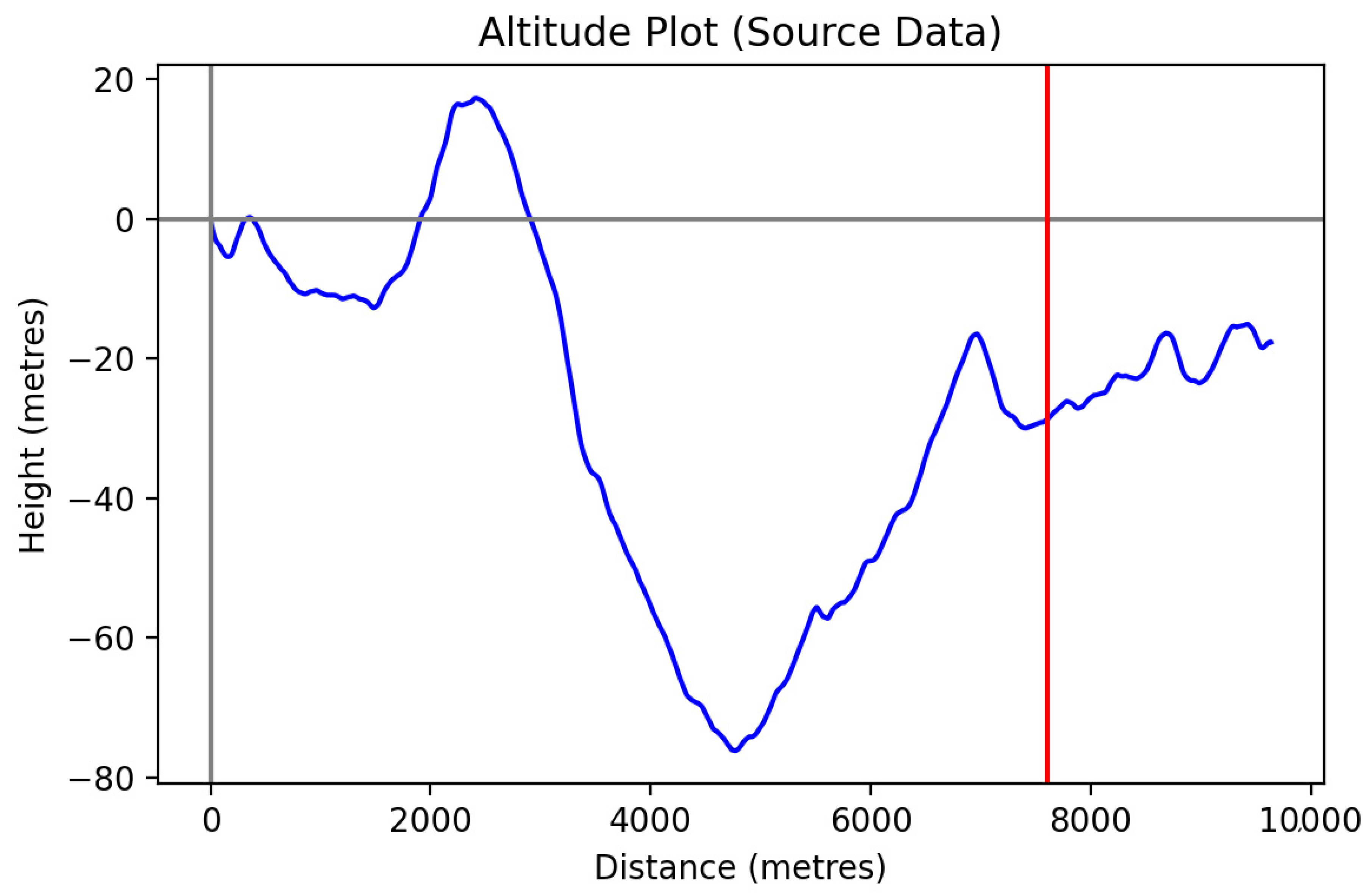
Finally, we apply the method to a real-life road gradient profile, as measured in the city of Lisbon. This is an interesting case due to the undulating terrain, and because the data used were part of the study that calibrated the power and energy relationships, as described in Section 2.1. A stretch of road was considered of a similar length to that considered in WMTC Reference Cycle 2 (see Section 2.2), for which the road profile is illustrated in 
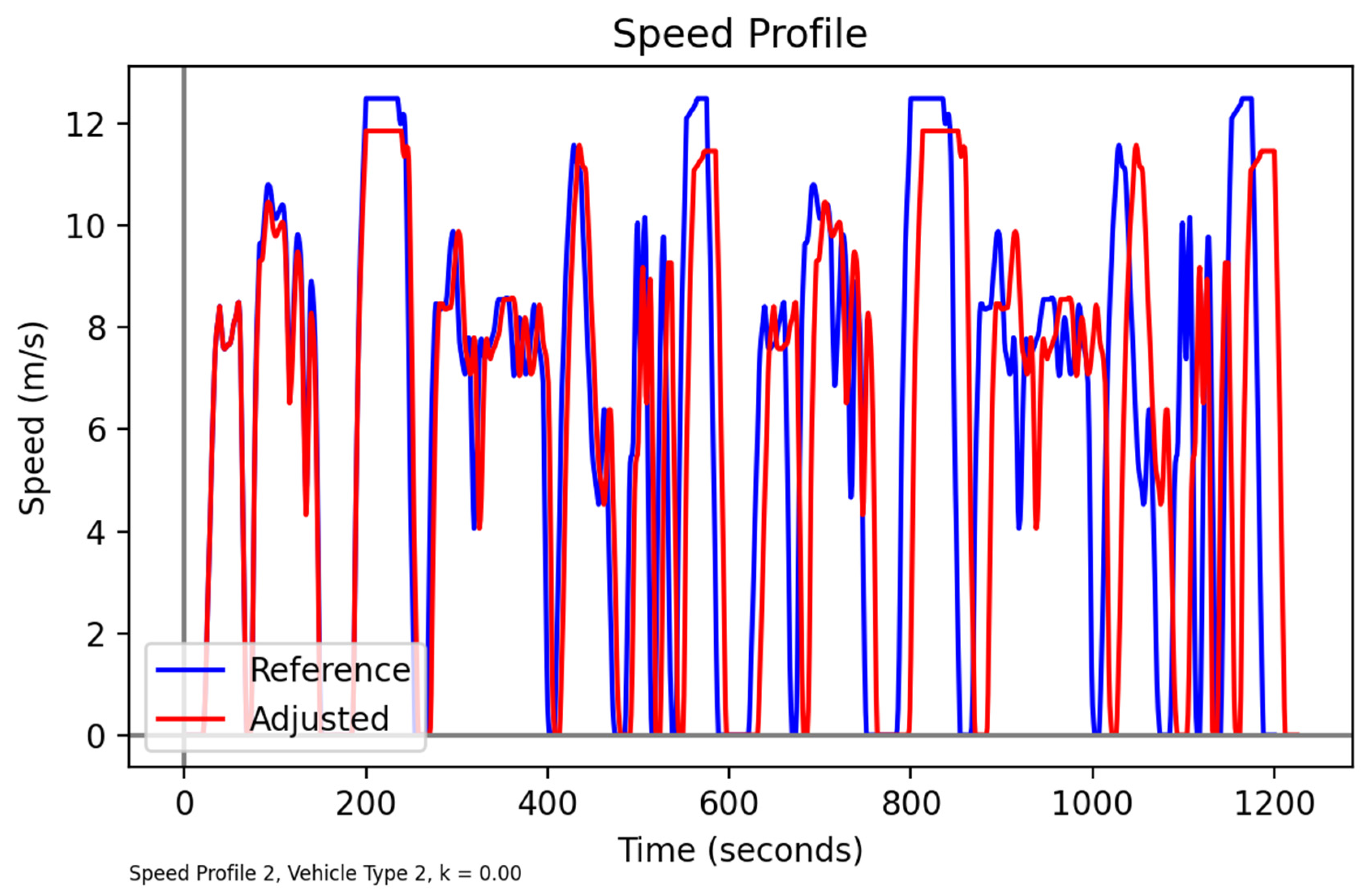
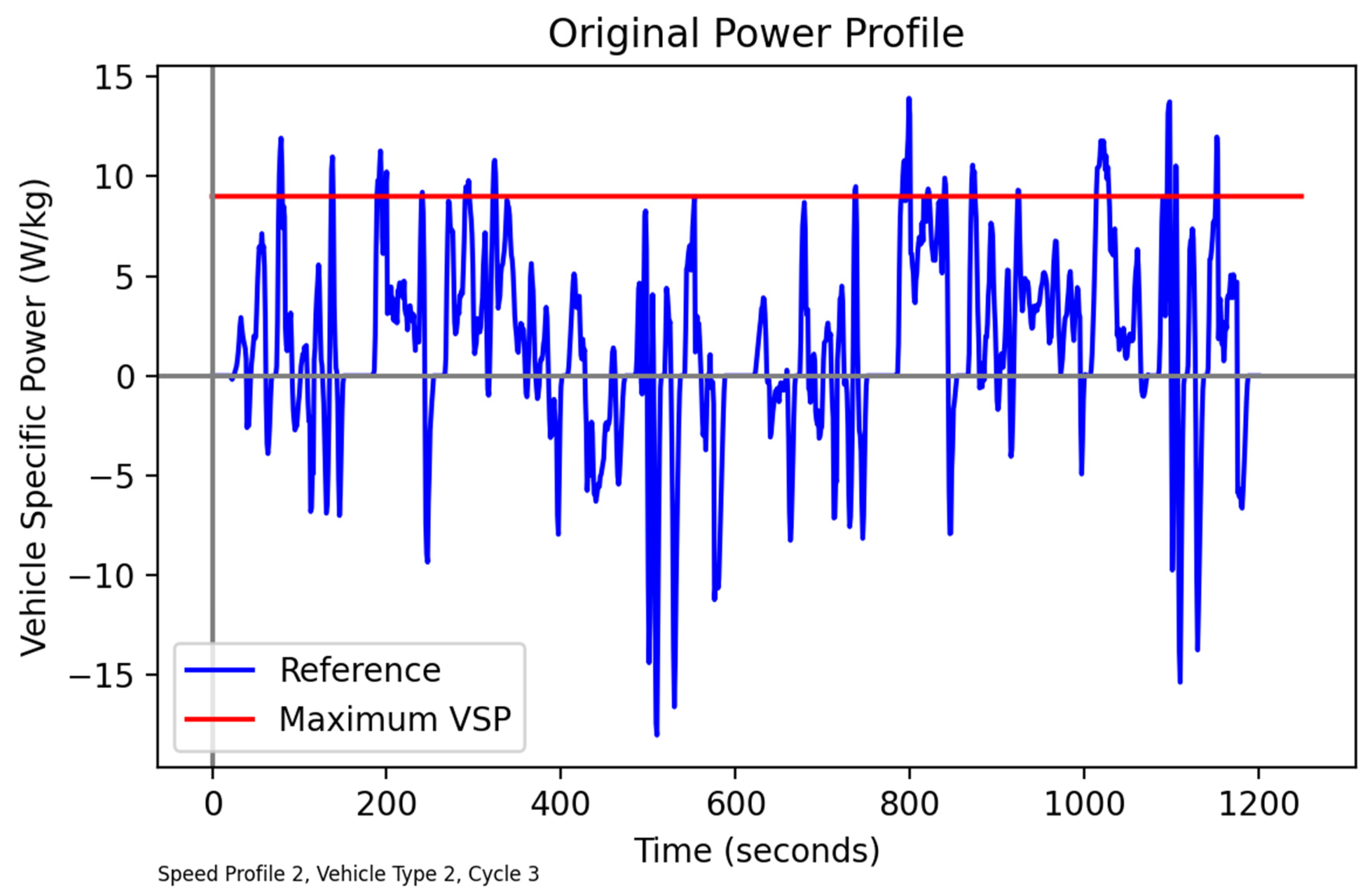
Figure 13. If the WMTC Reference Cycle 2 speeds are exactly followed, then the portion of the gradient up to the red line is used. Again considering Vehicle Type 2 (as defined in 
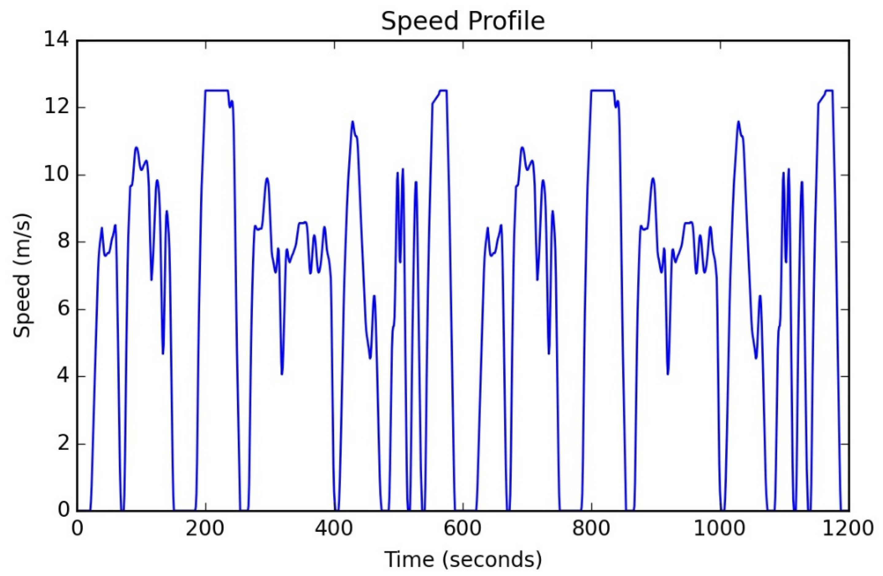
Table 7) and the WMTC reference speeds (
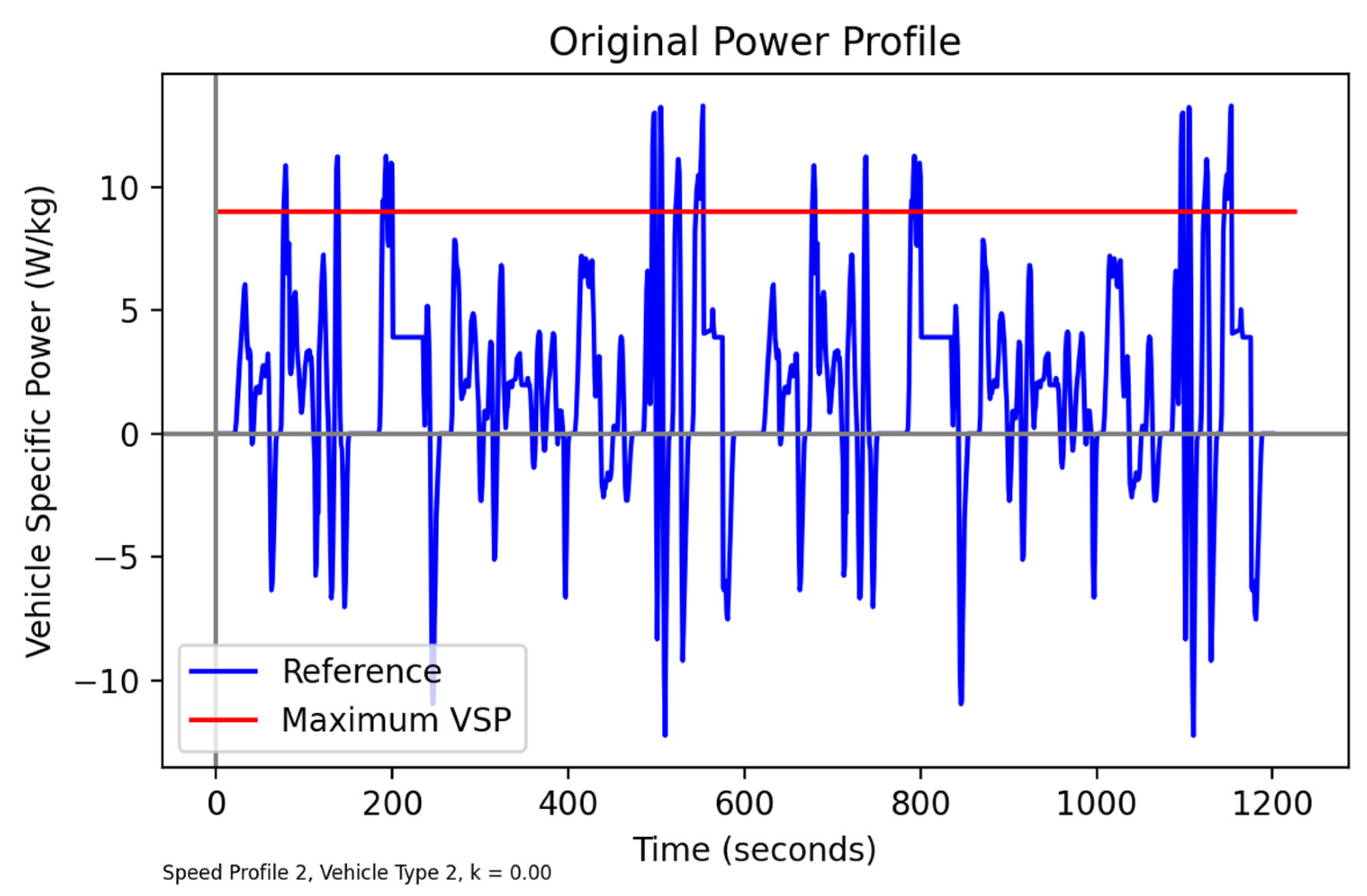
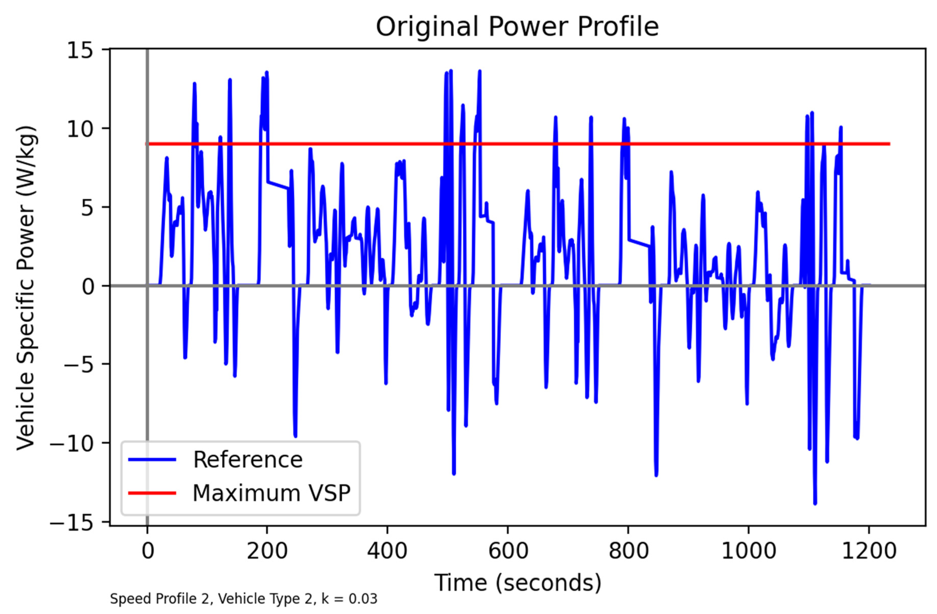
Figure 1), the resulting VSP profile (Figure 14) again shows violations of the maximum VSP, suggesting that the reference speed profile is not suited to this vehicle type and terrain. Applying the methodology described in 
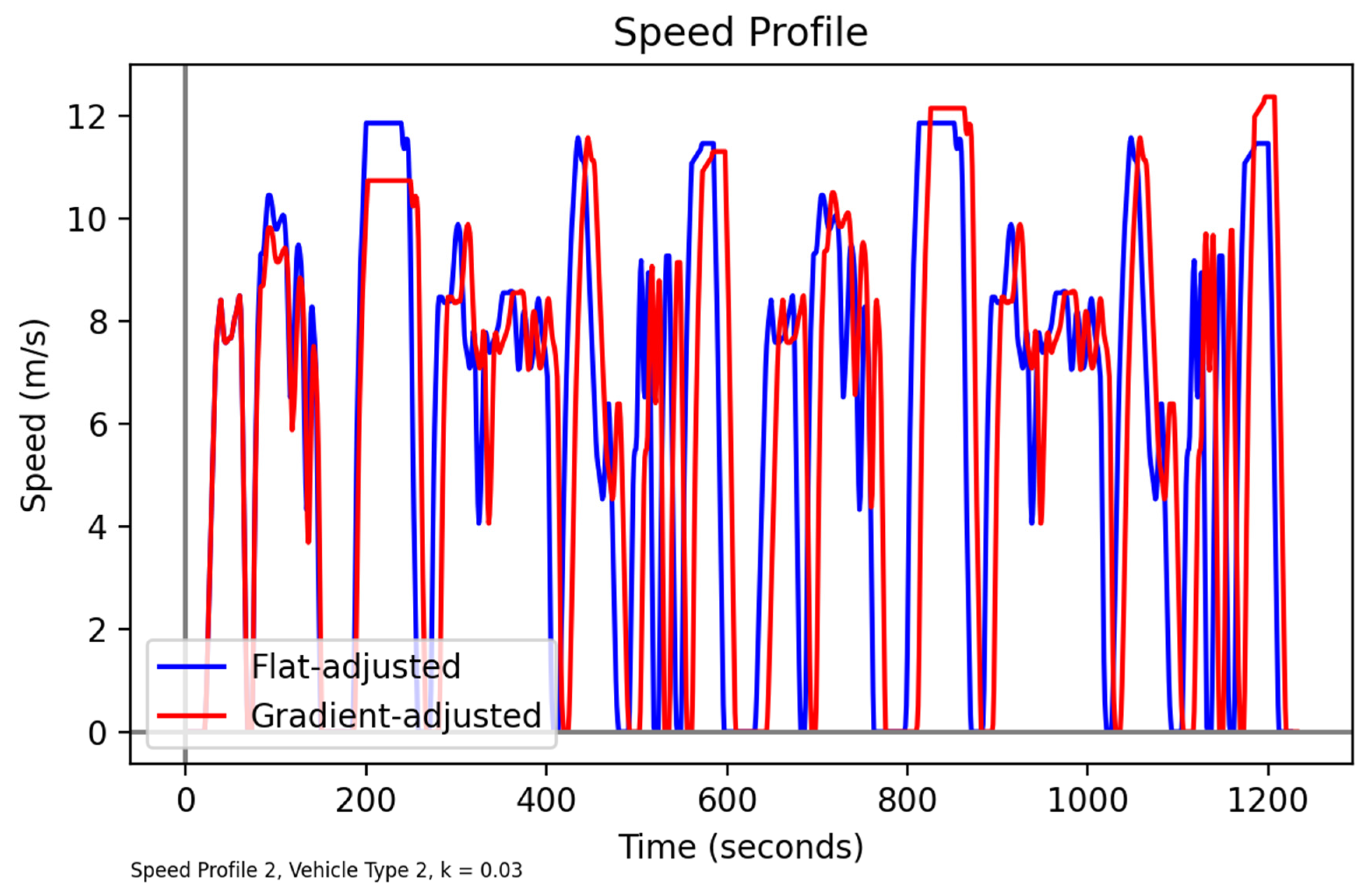
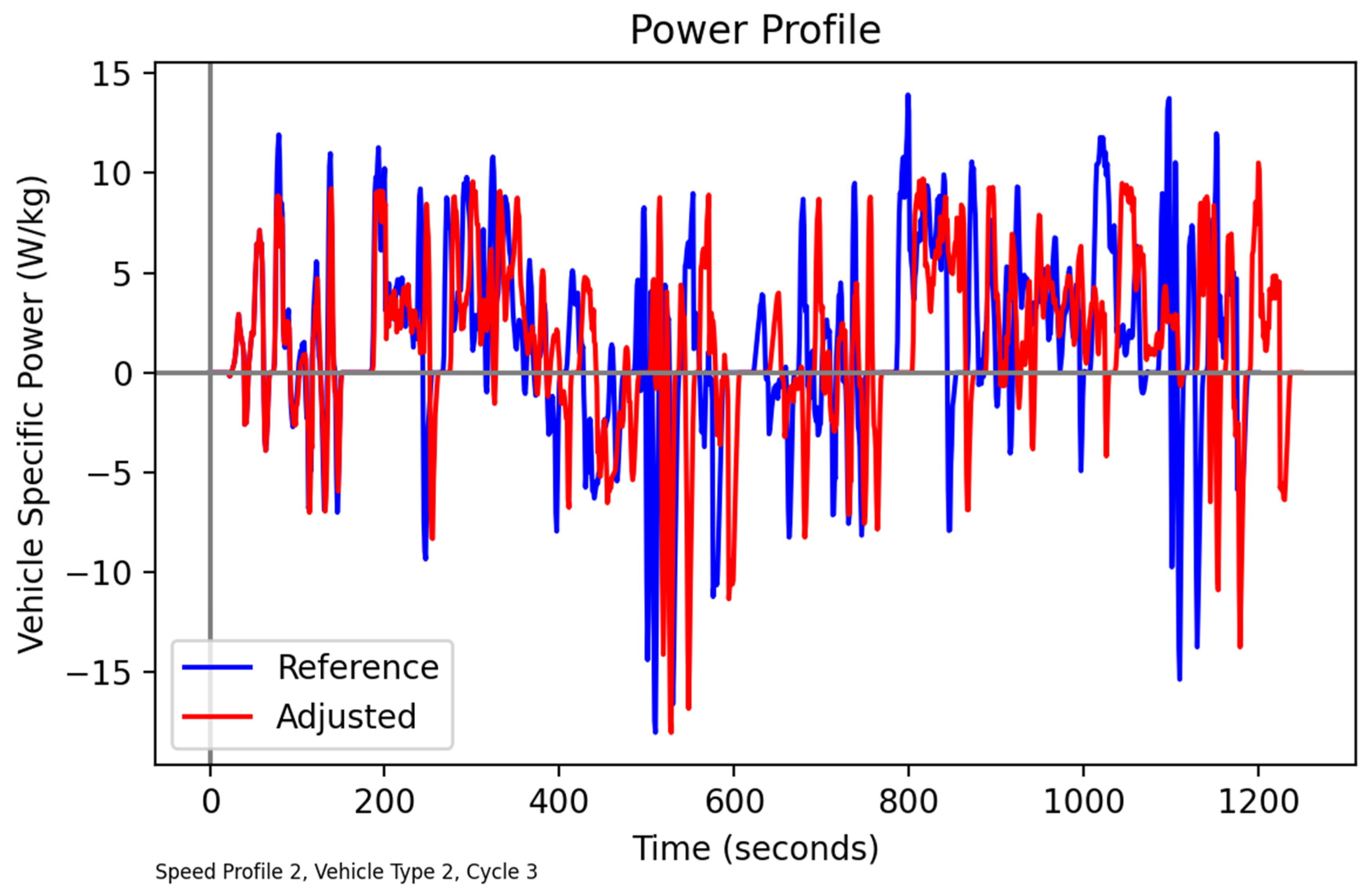
Section 3, a modified speed profile is produced (Figure 15). It is noticeable that, as would be anticipated, many of the speed modifications are associated with steeper uphill sections of the profile; for example, significant modifications are apparent towards the end of the cycle, corresponding to the final uphill section of 
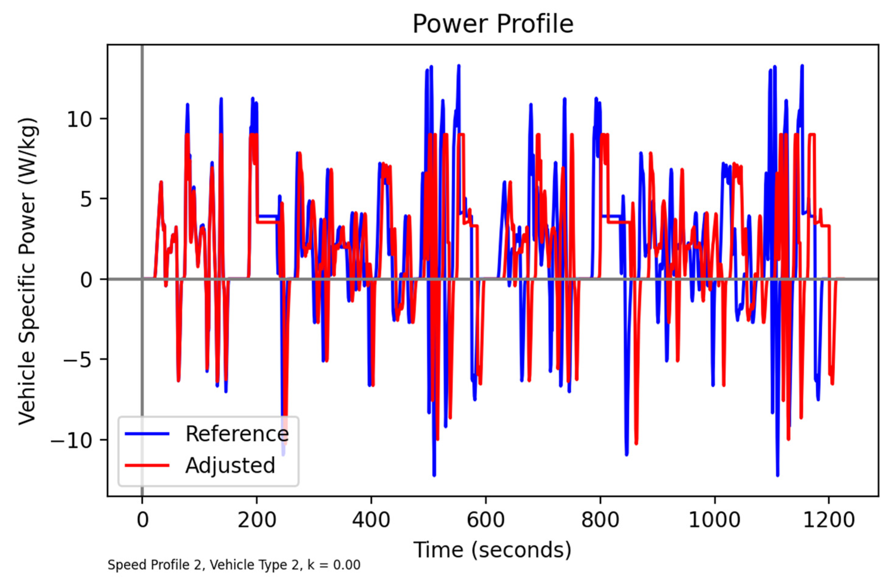
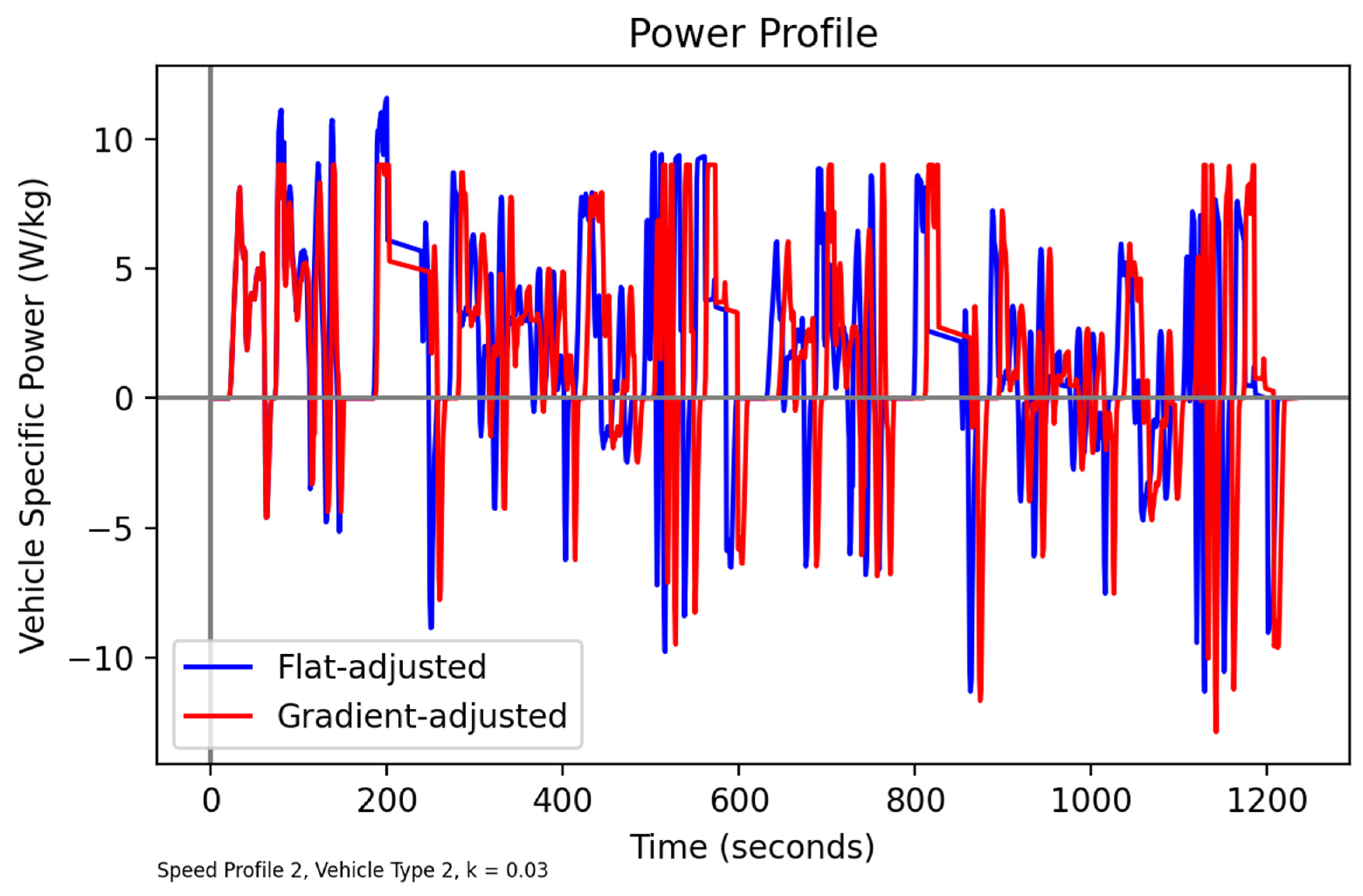
Figure 13. A comparison of the VSP profiles corresponding to the reference and modified speeds is given in 
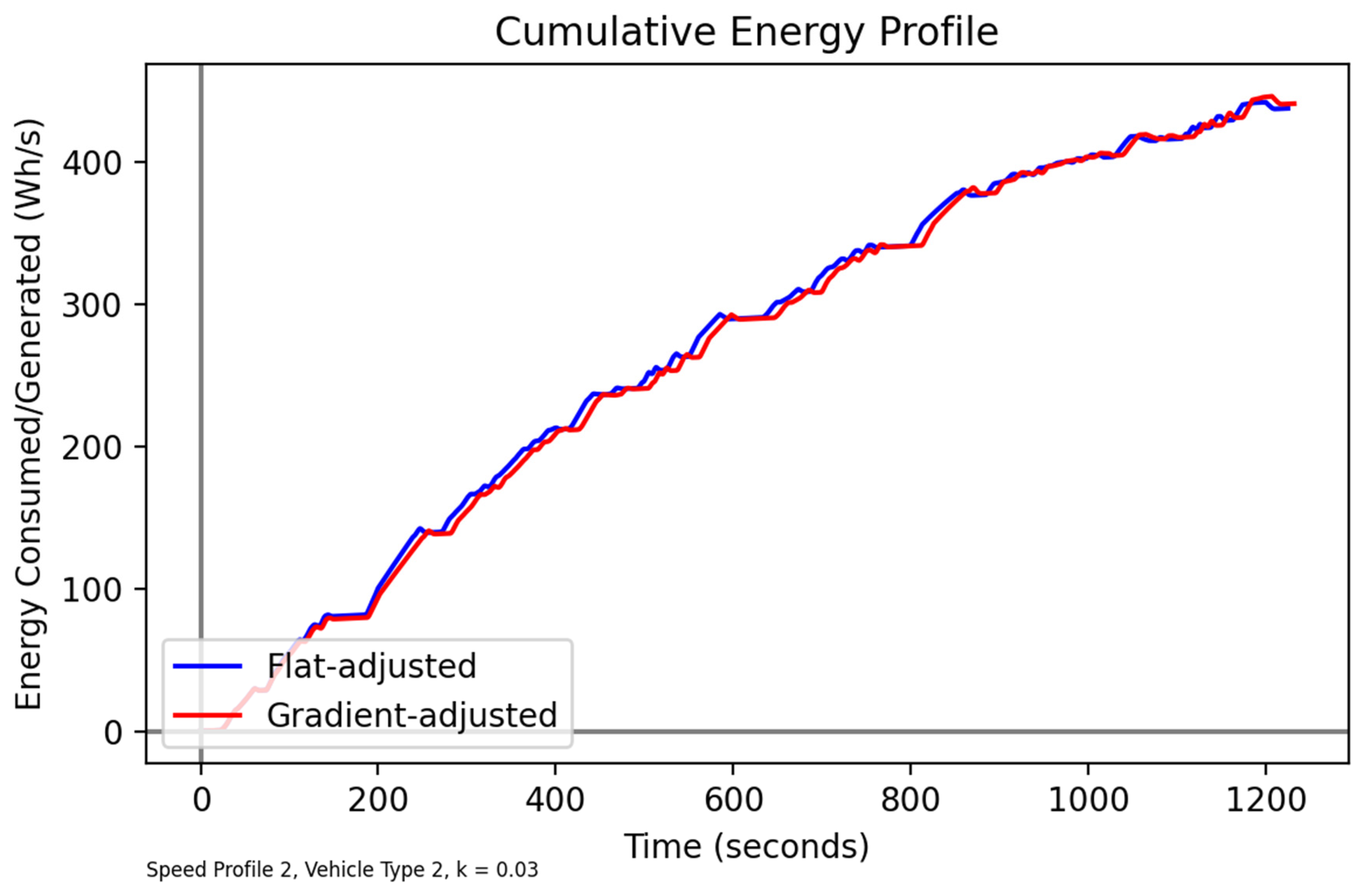
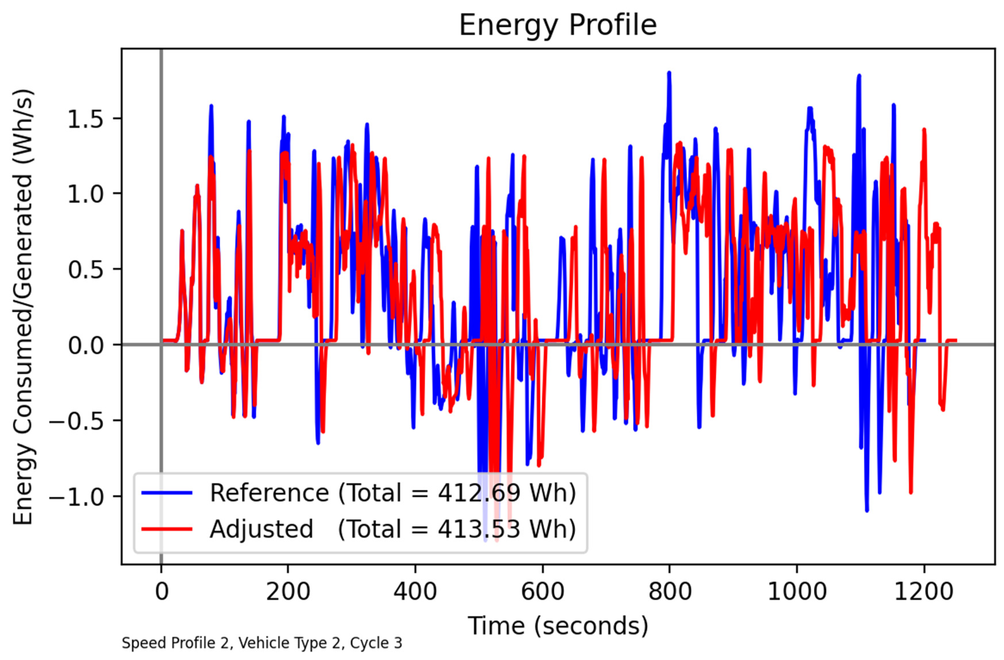
Figure 16, and confirms that the method is successful in constraining VSP to a feasible range, with the impacts on energy consumption depicted in Figure 17.
As a final experiment, we performed an analysis of the road slope in a forward and reversed direction, with the summary statistics for the original direction in Table 11 and Table 12, and for the reverse direction in Table 13 and Table 14. The adjusted results indicate a small difference of −0.8% in total travel time under the reverse topography compared with the original. However, at the same time, the total energy is reduced by 4.9%, regenerated energy decreases by 4.6%, while the percentage of time in a negative energy state increases by 6.5% for the reversed slope compared with the original topography. This suggests that the original road slope combined with the real-world cycle, after adjustment, is more energy demanding, but also produces higher energy from regeneration, although there are fewer opportunities to regenerate. Such a comparison demonstrates the complexity of real-world driving energy consumption on an L-category EV.

6. Conclusions

In the context of an expected emergence of L-category electric vehicles in the urban context, a generic methodology has been developed to adjust reference speed profiles to be applicable to the performance characteristics of these specific vehicles, while also accounting for different terrains. The methodology comprises three main elements: bounding maximum instantaneous power by dynamically limiting acceleration, given the current speed and gradient; bounding decelerations to avoid physically impossible speeds that may otherwise arise due to previous adjustments to speeds; and inserting cruising periods to ensure that the modified profile covers the same route length, albeit over a longer period of time.
The methodology has been applied, firstly, to derive speed profiles for electric quadricycles on flat terrain, given reference speed profiles for motorcycles. The results show that adjustments made to cope with the power limitations of L-EV do not introduce significant differences in energy consumption, suggesting that the certification does not require an extensive modification. Secondly, it was explored to what extent bespoke speed profiles are necessary for undulating terrain, as opposed to adopting the speed profiles developed for flat terrain in all cases. The first set of tests considered a fictitious road profile that was easily adjustable, namely a symmetric hill versus a symmetric valley. In this case, it was found that the power limitations, as well as the combination of a fixed driving profile and different magnitudes of slope and shapes of slope, lead to differences of up to 5% in energy use and of up to 10% in regenerated energy. The second set of tests analyzed the impact of topography on real-world driving cycles and slope (by considering a real-world profile driven in both directions), and qualitatively confirmed the results obtained for the fictitious profile tests.
The developed speed profiles are useful in their own right for studies that wish to assess the impacts of different measures and policies on electric quadricycles, with the advantage of considering regenerative capabilities and road grade, which are crucial in the characterization of energy performance in real-world conditions. The developed method may be readily extended to other L-category electric vehicles, given the relevant input information on vehicle specific power relations and maximum VSP.

Author Contributions

D.W.: conceptualization; formal analysis; methodology; software; writing—original draft. P.B.: formal analysis; writing—review & editing. G.D.: funding acquisition; formal analysis; writing—review & editing. J.G.: data curation. H.C.: funding acquisition; writing—review & editing. All authors have read and agreed to the published version of the manuscript.

Funding

The University of Leeds authors acknowledge the support of EU H2020-EU.3.4 funding, under grant agreement ID 769,926 for the project ELVITEN (elviten-project.eu). The IST-ID authors acknowledge the support of Fundação para a Ciência e Tecnologia for IN+ Strategic Project UID/EEA/50009/2019 and for contract CEECIND/02589/2017.

Institutional Review Board Statement

Not applicable.

Informed Consent Statement

Not applicable.

Data Availability Statement

This study did not report any new data. The reference cycles that were adapted can be found in reference [46]. All other parameter values used are reported in the main body of the current paper.

Conflicts of Interest

The authors declare no conflict of interest.

References

  1. Fulton, L.M. Three Revolutions in Urban Passenger Travel. Joule 2018, 2, 575–578. [Google Scholar] [CrossRef] [Green Version]
  2. Lee, R.; Brown, S. Evaluating the role of behavior and social class in electric vehicle adoption and charging demands. iScience 2021, 24, 102914. [Google Scholar] [CrossRef] [PubMed]
  3. Tushar, W.; Yuen, C.; Saha, T.; Chattopadhyay, D.; Nizami, S.; Hanif, S.; Alam, J.E.; Poor, H.V. Roles of Retailers in the Peer-to-Peer Electricity Market: A Single Retailer Perspective. iScience 2021, 24, 103278. [Google Scholar] [CrossRef]
  4. Fachrizal, R.; Shepero, M.; Van der Meer, D.; Munkhammar, J.; Widén, J. Smart charging of electric vehicles considering photovoltaic power production and electricity consumption: A review. eTransportation 2020, 4, 100056. [Google Scholar] [CrossRef]
  5. Transport & Environment. How Clean Are Electric Cars? 2020. Available online: https://www.transportenvironment.org/sites/te/files/downloads/T%26E%E2%80%99s%20EV%20life%20cycle%20analysis%20LCA_0.pdf (accessed on 3 February 2022).
  6. IEA. Global EV Outlook 2020: Entering the Decade of Electric Drive. 2020. Available online: https://www.iea.org/reports/global-ev-outlook-2020 (accessed on 3 February 2022).
  7. Zhang, H.; Zhang, J. An overview of modification strategies to improve LiNi0.8Co0.1Mn0.1O2 (NCM811) cathode performance for automotive lithium-ion batteries. eTransportation 2021, 7, 100105. [Google Scholar] [CrossRef]
  8. Santucci, M.; Pieve, M.; Pierini, M. Electric L-category vehicles for smart urban mobility. Transp. Res. Procedia 2016, 14, 3651–3660. [Google Scholar] [CrossRef] [Green Version]
  9. EU: Vehicle Categories. 2022. Available online: https://ec.europa.eu/growth/sectors/automotive-industry/vehicle-categories_en (accessed on 3 February 2022).
  10. Transportpolicy.net. EU: Vehicle Definitions. 2022. Available online: https://www.transportpolicy.net/standard/eu-vehicle-definitions/ (accessed on 3 February 2022).
  11. UNECE. Special Resolution No. 1 Concerning the Common Definitions of Vehicle Categories, Masses and Dimensions (S.R.1). World Forum for Harmonization of Vehicle Regulations, Report no. TRANS/WP.29/1045. 2005. Available online: https://unece.org/classification-and-definition-vehicles (accessed on 3 February 2022).
  12. Ewert, A.; Brost, M.; Eisenmann, C.; Stieler, S. Small and Light Electric Vehicles: An Analysis of Feasible Transport Impacts and Opportunities for Improved Urban Land Use. Sustainability 2020, 12, 8098. [Google Scholar] [CrossRef]
  13. Ministry of Road Transport and Highways. Gazette of India: Extraordinary, Part II Section 3, Sub-Section (i). 2014. Available online: https://morth.nic.in/sites/default/files/notifications_document/Notification_No_GSR_99E_dated_1922014%C2%A0.pdf (accessed on 3 February 2022).
  14. Korean Transportation Safety Authority. Korean Safety Regulations on Micro Mobility Related to Passive Safety. Informal Document GRSP-65-23. 2019. Available online: https://unece.org/DAM/trans/doc/2018/wp29grsp/GRSP-65-23e.pdf (accessed on 3 February 2022).
  15. National Highway Traffic Safety Administration. Federal Motor Vehicle Safety Standards: Low-Speed Vehicles. US Federal Register, Document Number 06-3590. 2006. Available online: https://www.federalregister.gov/documents/2006/04/19/06-3590/federal-motor-vehicle-safety-standards-low-speed-vehicles (accessed on 3 February 2022).
  16. Pavlovic, A.; Fragassa, C. General considerations on regulations and safety requirements for quadricycles. Int. J. Qual. Res. 2015, 9, 657–674. [Google Scholar]
  17. EEA. The First and Last Mile; European Environment Agency: Copenhagen, Denmark, 2019.
  18. Martiskainen, M.; Sovacool, B.K.; Lacey-Barnacle, M.; Hopkins, D.; Jenkins, K.E.H.; Simcock, N.; Mattioli, G.; Bouzarovski, S. New dimensions of vulnerability to energy and transport poverty. Joule 2021, 5, 3–7. [Google Scholar] [CrossRef]
  19. Sachs, C.; Burandt, S.; Mandelj, S.; Mutter, R. Assessing the market of light electric vehicles as a potential application for electric in-wheel drives. In Proceedings of the IEEE 6th International Electric Drives Production Conference (EDPC), Nuremberg, Germany, 30 November–1 December 2016; pp. 280–285. [Google Scholar]
  20. Renault. Renault Twizy E-tech Electric. 2021. Available online: https://www.renault.pt/veiculos-eletricos/twizy.html (accessed on 3 February 2022).
  21. Citröen. My Ami Orange. 2021. Available online: https://www.citroen.pt/ami (accessed on 3 February 2022).
  22. EU. Sustainable and Smart Mobility Strategy—Putting European Transport on Track for the Future. Communication from the Commission to the European Parliament, The Council, The European Economic and Social Committee and the Committee of the Regions. 2020. Available online: https://eur-lex.europa.eu/legal-content/EN/TXT/HTML/?uri=CELEX:52020DC0789&from=EN (accessed on 3 February 2022).
  23. Alves, J.; Baptista, P.C.; Gonçalves, G.A.; Duarte, G.O. Indirect methodologies to estimate energy use in vehicles: Application to battery electric vehicles. Energy Convers. Manag. 2016, 124, 116–129. [Google Scholar] [CrossRef]
  24. Fiori, C.; Ahn, K.; Rakha, H.A. Power-based electric vehicle energy consumption model: Model development and validation. Appl. Energy 2016, 168, 257–268. [Google Scholar] [CrossRef]
  25. Luin, B.; Petelin, S.; Al-Mansour, F. Microsimulation of electric vehicle energy consumption. Energy 2019, 174, 24–32. [Google Scholar] [CrossRef]
  26. Xie, Y.; Li, Y.; Zhao, Z.; Dong, H.; Wang, S.; Liu, J.; Guan, J.; Duan, X. Microsimulation of electric vehicle energy consumption and driving range. Appl. Energy 2020, 267, 115081. [Google Scholar] [CrossRef]
  27. Zhang, J.; Wang, Z.; Liu, P.; Zhang, Z.; Li, X.; Qu, C. Driving cycles construction for electric vehicles considering road environment: A case study in Beijing. Appl. Energy 2019, 253, 113514. [Google Scholar] [CrossRef]
  28. Chiang, H.L.; Huang, P.H.; Lai, Y.M.; Lee, T.Y. Comparison of the regulated air pollutant emission characteristics of real-world driving cycle and ECE cycle for motorcycles. Atmos. Environ. 2014, 87, 1–9. [Google Scholar] [CrossRef]
  29. Tutuianu, M.; Bonnel, P.; Ciuffo, B.; Haniu, T.; Ichikawa, N.; Marotta, A.; Pavlovic, J.; Steven, H. Development of the World-wide harmonized Light duty Test Cycle (WLTC) and a possible pathway for its introduction in the European legislation. Transp. Res. Part D Transp. Environ. 2015, 40, 61–75. [Google Scholar] [CrossRef]
  30. Giechaskiel, B.; Zardini, A.; Martini, G. Particle emission measurements from L-category vehicles. SAE Int. J. Engines 2015, 8, 2322–2337. [Google Scholar] [CrossRef]
  31. Burrows, A. EU Regulation on the Approval of L-Category Vehicles. 2013. Available online: https://www.zemo.org.uk/assets/presentations/EU%20Regulation%20on%20the%20Approval%20of%20L-Category%20Vehicles.pdf (accessed on 3 February 2022).
  32. RESOLVE. Range of Electric Solutions for L-Category Vehicles. 2018. Available online: http://www.resolve-project.eu/ (accessed on 3 February 2022).
  33. Kamble, S.H.; Mathew, T.V.; Sharma, G.K. Development of real-world driving cycle: Case study of Pune, India. Transp. Res. Part D Transp. Environ. 2009, 14, 132–140. [Google Scholar] [CrossRef]
  34. Al-Wreikat, Y.; Serrano, C.; Sodré, J.R. Driving behaviour and trip condition effects on the energy consumption of an electric vehicle under real-world driving. Appl. Energy 2021, 297, 117096. [Google Scholar]
  35. Kühne, R. Electric buses—An energy efficient urban transportation means. Energy 2010, 35, 4510–4513. [Google Scholar] [CrossRef]
  36. Schücking, M.; Jochem, P. Two-stage stochastic program optimizing the cost of electric vehicles in commercial fleets. Appl. Energy 2021, 293, 116649. [Google Scholar] [CrossRef]
  37. Welzel, F.; Klinck, C.-F.; Pohlmann, Y.; Bednarczyk, M. Grid and user-optimized planning of charging processes of an electric vehicle fleet using a quantitative optimization model. Appl. Energy 2021, 290, 116717. [Google Scholar] [CrossRef]
  38. Jiménez-Palacios, J.L. Understanding and Quantifying Motor Vehicle Emissions with Vehicle Specific Power and TILDAS Remote-Sensing. Ph.D. Thesis, Massachusetts Institute of Technology, Massachusetts, MA, USA, 1999. [Google Scholar]
  39. Frey, H.C.; Rouphail, N.M.; Zhai, H.; Farias, T.L.; Gonçalves, G.A. Comparing real-world fuel consumption for diesel- and hydrogen-fueled transit buses and implication for emissions. Transp. Res. Part D 2007, 12, 281–291. [Google Scholar] [CrossRef]
  40. Frey, H.; Unal, A.; Rouphail, N.; Colyar, J. On-road measurement of vehicle tailpipe emissions using a portable instrument. J. Air Waste Manag. Assoc. 2003, 53, 992–1002. [Google Scholar] [CrossRef] [Green Version]
  41. Rhys-Tyler, G.; Bell, M. Toward reconciling instantaneous roadside measurements of LDV exhaust emission with type approval driving cycles. Environ. Sci. Technol. 2012, 46, 10532–10538. [Google Scholar] [CrossRef] [Green Version]
  42. Duarte, G.O.; Gonçalves, G.A.; Baptista, P.C.; Farias, T.L. Establishing bonds between vehicle certification data and real-world vehicle fuel consumption—A vehicle specific power approach. Energy Convers. Manag. 2015, 92, 251–265. [Google Scholar] [CrossRef]
  43. Varella, R.; Duarte, G.; Baptista, P.; Sousa, L.; Villafuerte, P.M. Comparison of Data Analysis Methods for European Real Driving Emissions Regulation; SAE Technical Paper 2017-01-0997; SAE International: Warrendale, PA, USA, 2017. [Google Scholar] [CrossRef]
  44. Aprillia, H.; Yang, H.-T.; Huang, C.-M. Optimal Decomposition and Reconstruction of Discrete Wavelet Transformation for Short-Term Load Forecasting. Energies 2019, 12, 4654. [Google Scholar] [CrossRef] [Green Version]
  45. Shi, P.; Yang, W.; Sheng, M.; Wang, M. An Enhanced Empirical Wavelet Transform for Features Extraction from Wind Turbine Condition Monitoring Signals. Energies 2017, 10, 972. [Google Scholar] [CrossRef] [Green Version]
  46. EU. Reglamento Delegado (UE) No. 134/2014 de la Comisión. Consolidated Text: Commission Delegated Regulation (EU) No. 134/2014 of 16 December 2013 Supplementing Regulation (EU) No. 168/2013 of the European Parliament and of the Council with Regard to Environmental and Propulsion Unit Performance Requirements and Amending Annex V Thereof. 2013. Available online: http://data.europa.eu/eli/reg_del/2014/134/2018-03-20 (accessed on 3 February 2022).
Figure 1. Speed profile from WMTC Reference Cycle 2.
Energies 15 03466 g001
Figure 2. Implied Vehicle Specific Power for an electric quadricycle following speed profile stipulated in WMTC Reference Cycle 2 (Flat terrain).
Energies 15 03466 g002
Figure 3. Implied vehicle-specific power for an electric quadricycle following the acceleration profile stipulated in WMTC Reference Cycle 2 (Hilly terrain, k = 0.03).
Energies 15 03466 g003
Figure 4. Schematic representation of the applied methodology.
Energies 15 03466 g004
Figure 5. Adjusted speed profile for electric quadricycle in comparison with reference cycle (WMTC Reference Cycle 1, Vehicle Type 2, Flat terrain assumed in adjustment).
Energies 15 03466 g005
Figure 6. Adjusted speed profile for electric quadricycle in comparison with reference cycle (WMTC Reference Cycle 2, Vehicle Type 2, Flat terrain assumed in adjustment).
Energies 15 03466 g006
Figure 7. Distance travelled as a function of time for adjusted and reference speed profiles (WMTC Reference Cycle 2, Vehicle Type 2, Flat terrain assumed in adjustment).
Energies 15 03466 g007
Figure 8. Vehicle Specific Power profile for adjusted and reference speed profiles (WMTC Reference Cycle 2, Vehicle Type 2, Flat terrain assumed in adjustment).
Energies 15 03466 g008
Figure 9. Acceleration profile for adjusted and reference speed profiles (WMTC Reference Cycle 2, Vehicle Type 2, Flat terrain assumed in adjustment).
Energies 15 03466 g009
Figure 10. Comparison of adjusted speed profiles for Flat (k = 0) and Gradient (k = 0.03) cases (Both adjusted from WMTC Reference Cycle 2; Vehicle Type 2).
Energies 15 03466 g010
Figure 11. Comparison of VSP profiles following Flat (k = 0) vs. Gradient (k = 0.03) adjusted speed profiles, both evaluated on k = 0.03 terrain (Both adjusted from WMTC Reference Cycle 2; Vehicle Type 2).
Energies 15 03466 g011
Figure 12. Comparison of cumulative energy profiles for Flat (k = 0) vs. Gradient (k = 0.03) adjusted speed profiles, both evaluated on k = 0.03 terrain (Both adjusted from WMTC Reference Cycle 2; Vehicle Type 2).
Energies 15 03466 g012
Figure 13. Studied road profile for Lisbon case study.
Energies 15 03466 g013
Figure 14. VSP profile obtained from applying WMTC Speed Profile 2 to the Lisbon case.
Energies 15 03466 g014
Figure 15. Reference and adjusted speed profiles for the Lisbon case.
Energies 15 03466 g015
Figure 16. VSP under reference and adjusted speed profiles for the Lisbon case.
Energies 15 03466 g016
Figure 17. Energy consumption under reference and adjusted speed profiles for the Lisbon case.
Energies 15 03466 g017
Table 1. Specification of test vehicles.
VehicleDimensions (m)
Length; Width; Height
Total Weight w/Batteries (kg)Max. Power (kW)Motor TechnologyBattery Technology
Type 1 1.74; 1.03; 1.573704DCPb-Acid
Type 22.40; 1.03; 1.504004DCPb-Acid
Type 32.63; 1.32; 1.515658AC inductionPb-Acid
Table 2. Estimated coefficients for relationship between ECR and VSP for three types of quadricycle.
β 1   β 2   β 3   β 4   β 5   β 6   β 7   β 8  
Type 10.120670.251920.047650.117590.02083−0.020560.023110.02083
Type 20.11010.268340.045260.116210.02778−0.020390.023790.02778
Type 30.190950.160020.059730.107720.05556−0.034270.041070.05556
Table 3. Kinetic summary statistics of adjusted drive cycles (WMTC Cycle 1).
ProfileSpeed (m/s)Positive Acceleration (m/s2)Negative Acceleration (m/s2)Total Idling Time (s)Total Travel Time (s)
MeanMaxMeanMaxMeanMax
Reference4.896.940.601.64−0.44 −1.66185.01201.0
Type 1 Adjusted4.876.940.601.64−0.44−1.66185.01206.7
Type 2 Adjusted4.876.940.601.64−0.44−1.66185.01206.7
Type 3 Adjusted4.876.940.601.64−0.44−1.66185.01206.7
Table 4. Energy-related summary statistics of adjusted drive cycles (WMTC Cycle 1).
VehicleProfileTotal Energy (Wh)Regenerated Energy (Wh)% Time in Negative Energy State% Time in Positive Energy State
Type 1Reference296.1921.938.4991.42
Adjusted294.6821.528.4691.46
Type 2Reference293.9521.037.9991.92
Adjusted292.6020.637.9691.96
Type 3Reference361.2934.477.9991.92
Adjusted361.2934.477.9991.92
Table 5. Kinetic summary statistics of adjusted drive cycles (WMTC Cycle 2).
ProfileSpeed (m/s)Positive Acceleration (m/s2)Negative Acceleration (m/s2)Total Idling Time (s)Total Travel Time (s)
MeanMaxMeanMaxMeanMax
Reference6.3312.500.461.64−0.55−1.74227.01201.00
Type 1 Adjusted6.2011.870.441.64−0.54−1.74233.01226.14
Type 2 Adjusted6.2011.870.441.64−0.54−1.74233.01226.14
Type 3 Adjusted6.3212.500.461.64−0.55−1.74227.01203.22
Table 6. Energy-related summary statistics of adjusted drive cycles (WMTC Cycle 2).
VehicleProfileTotal Energy (Wh)Regenerated Energy (Wh)% Time in Negative Energy State% Time in Positive Energy State
Type 1Reference460.6552.8616.6583.26
Adjusted456.4647.5715.8284.09
Type 2Reference445.2350.7615.6584.26
Adjusted442.6445.6514.8585.07
Type 3Reference587.8383.2815.6584.26
Adjusted586.5982.3815.6384.29
Table 7. Total energy consumption (Wh) under alternative speed profiles, gradient assumptions, and vehicle types (symmetric hill, WMTC Reference Cycle 2).
Vehicle Type 1Vehicle Type 2Vehicle Type 3
k0.010.030.050.010.030.050.010.030.05
Reference463.9462.0457.1448.2445.5439.1591.5594.9597.7
Flat adj speed457.5452.4449.4443.5437.5432.8591.2593.6596.6
Grad adj speed458.59455.5454.2444.5440.8438.2590.8593.0593.9
Table 8. Percentage of regenerative energy under alternative speed profiles, gradient assumptions, and vehicle types (symmetric hill, WMTC Reference Cycle 2).
Vehicle Type 1Vehicle Type 2Vehicle Type 3
k0.010.030.050.010.030.050.010.030.05
Reference11.6512.4914.4211.5812.4314.3914.3915.2517.31
Flat adj speed10.6311.4713.4810.5211.3713.4014.2615.1317.19
Grad adj speed10.6411.5913.4510.5311.4813.3414.3015.1317.08
Table 9. Total energy consumption (Wh) under alternative speed profiles, gradient assumptions, and vehicle types (symmetric valley, WMTC Reference Cycle 2).
Vehicle Type 1Vehicle Type 2Vehicle Type 3
k−0.01−0.03−0.05−0.01−0.03−0.05−0.01−0.03−0.05
Reference458.9446.4447.1443.5430.5429.6586.7579.6588.9
Flat adj speed458.6439.5443.0444.7425.1427.7585.5578.3587.7
Grad adj speed460.2441.1443.1446.3426.9427.7584.9576.8583.8
Table 10. Percentage of regenerative energy under alternative speed profiles, gradient assumptions, and vehicle types (symmetric valley, WMTC Reference Cycle 2).
Vehicle Type 1Vehicle Type 2Vehicle Type 3
k−0.01−0.03−0.05−0.01−0.03−0.05−0.01−0.03−0.05
Reference11.3711.9213.0811.2811.8613.0313.9814.4515.56
Flat adj speed10.2610.9712.1510.1510.8712.0513.8714.3615.47
Grad adj speed10.1810.9212.1010.0710.8211.9913.8314.2415.36
Table 11. Kinetic summary statistics under reference and adjusted speed profiles for the Lisbon case.
ProfileSpeed (m/s)Positive Acceleration (m/s2)Negative Acceleration (m/s2)Total Idling Time (s)Total Travel Time (s)
MeanMaxMeanMaxMeanMax
Reference6.3312.500.461.64−0.55−1.74227.01201.00
Adjusted6.0812.500.441.64−0.55−1.73237.01250.89
Table 12. Energy-related summary statistics under reference and adjusted speed profiles for the Lisbon case.
ProfileTotal Energy (Wh)Regenerated Energy (Wh)% Time in Negative Energy State% Time in Positive Energy State
Reference428.6775.3221.8278.10
Adjusted427.7871.4621.4478.48
Table 13. Kinetic summary statistics under reference and adjusted speed profiles for the Lisbon case with reversed road profile.
ProfileSpeed (m/s)Positive Acceleration (m/s2)Negative Acceleration (m/s2)Total Idling Time (s)Total Travel Time (s)
MeanMaxMeanMaxMeanMax
Reference6.3312.500.461.64−0.55−1.74227.01201.00
Adjusted6.1311.720.431.63−0.53−1.73238.01240.42
Table 14. Energy-related summary statistics under reference and adjusted speed profiles for the Lisbon case with reversed road profile.
ProfileTotal Energy (Wh)Regenerated Energy (Wh)% Time in Negative Energy State% Time in Positive Energy State
Reference411.9574.1924.4075.52
Adjusted406.5968.1622.8477.08
Publisher’s Note: MDPI stays neutral with regard to jurisdictional claims in published maps and institutional affiliations.

