Multiple Power Supply Capacity Planning Research for New Power System Based on Situation Awareness

Abstract

In the context of new power systems, reasonable capacity optimization of multiple power systems can not only reduce carbon emissions, but also improve system safety and stability. This paper proposes a situation awareness-based capacity optimization strategy for wind-photovoltaic-thermal power systems and establishes a bi-level model for system capacity optimization. The upper-level model considers environmental protection and economy, and carries out multi-objective optimization of the system capacity planning solution with the objectives of minimizing carbon emissions and total system cost over the whole life cycle of the system, further obtaining a set of capacity planning solutions based on the Pareto frontier. A Pareto optimal solution set decision method based on grey relativity analysis is proposed to quantitatively assess the comprehensive economic–environmental properties of the system. The capacity planning solutions obtained from the upper model are used as the input to the lower model. The lower model integrates system stability, environmental protection, and economy and further optimizes the set of capacity planning solutions obtained from the upper model with the objective of maximizing the inertia security region and the best comprehensive economic–environmental properties to obtain the optimal capacity planning scheme. The NSGA-II modified algorithm (improved NSGA-II algorithm based on dominant strength, INSGA2-DS) is used to solve the upper model, and the Cplex solver is called on to solve the lower model. Finally, the modified IEEE-39 node algorithm is used to verify that the optimized capacity planning scheme can effectively improve the system security and stability and reduce the carbon emissions and total system cost throughout the system life cycle.

1. Introduction

In the context of the new power system, with the increased development of new energy generation, the proportion of wind power and photovoltaic integrated into the grid has been increasing year by year. The wind-photovoltaic-thermal power system can effectively bring into play the complementary characteristics and synergistic effects of different forms of energy, improve the level of new energy consumption within a certain range, and achieve the purpose of making full use of energy resources. Reasonable system capacity planning is the basis for the safe and stable operation of the system.

A great deal of research has been done by domestic and international scholars on the planning of power systems containing renewable energy. The paper [1] assesses the impact of regional and international renewable energy policy coordination on the economics, environmental performance, and planning outcomes of the North American power sector in the context of renewable energy policy coordination and identifies the need to integrate cost, emissions, trade, and infrastructure investment in future capacity planning decisions for renewable energy-containing power systems through a multi-model comparison analysis using multiple energy-economic models. The literature [2] proposes a modeling approach adapted to the planning of power systems containing renewable energy sources while dividing the modeling approach into four categories and concluding that the choice of model should depend on the purpose of the study as well as the system characteristics. It provides a reference value for the research on the planning of power systems containing renewable energy.

Most of the existing studies on multiple power supply planning have been considered in terms of economics and environmental protection. The literature [3] investigates the capacity configuration of scenic power generation systems by using data, such as network node voltage and scenic power output, through a nuclear limit learning machine method to find the solution that minimizes the total investment cost and network losses. The paper [4] takes into account the environmental factors and takes the CO₂ emission of the whole life cycle of the wind and solar power system as the optimization target to optimize the capacity allocation of the wind and solar power system. The literature [5] considers the construction and maintenance costs, energy wastage, and outage losses of wind-complementary microgrids, and obtains an optimal allocation model that matches the meteorological conditions to optimize the capacity allocation of wind-complementary islanded microgrids. The literature [6] uses the lowest operating cost and the lowest system grid power supply rate as the optimization objectives for rational planning of the configuration of integrated energy systems, including wind power and photovoltaic power generation. A multi-objective optimization model with the objectives of minimizing total investment, node voltage exceedance probability, and undersupply probability was developed in [7]. An improved parallel elite non-dominated ranking genetic algorithm II is used to search for the Pareto optimal configuration solution for the optimal configuration of the wind and solar complementary system. The literature [8] investigates the optimization of wind capacity in power systems, considering system operation, economy, and reliability. The assessment of the economic aspects is obtained based on the social cost of the whole system, and the probabilistic method is used to assess the reliability of the system load loss probability. The planning problem of wind power capacity is solved through an opportunity-constrained planning approach. The literature [9,10] investigates the assessment of power system flexibility for the problem of planning systems with a high penetration of renewable energy sources, such as photovoltaic power. The concept of flexibility is reviewed and indicators for assessing the flexibility of power systems are summarised.

The above literature provides a reference for the study of multiple power supply planning in the context of new power systems but lacks consideration of system stability.

With the massive penetration of new energy sources, the inertia support of the system under active disturbance is severely weakened and the problem of inertia reduction cannot be ignored. Domestic and international new energy high percentage power grids have repeatedly experienced inertia shortages in operation, with significant frequency stability problems, thus exposing the system to the risk of large area cut-offs and load shedding.

At this stage, most of the research on system inertia presents an inertia assessment problem. The literature [11] describes the concept, characteristics, and assessment methods of the inertia security region. Literature [12] introduces the concept of minimum inertia demand for microgrids, establishes a minimum inertia demand assessment model, and proposes an optimal solution method. [13] proposes a method for estimating system inertia based on electromechanical oscillation parameters driven by stochastic data. Few studies have considered the impact on the optimal allocation of wind-photovoltaic-thermal power system capacity by taking the system inertia security region as an objective function.

Situation awareness is a technique for acquiring, understanding, and predicting the activities of elements that can cause changes in the system’s situation [14]. Currently, situation awareness techniques are gradually being applied in the field of power systems [15].

Capacity planning involves finding the best capacity planning solution for building generation capacity subject to various economic and technical constraints. In the face of today’s stricter environmental policies and increasing uncertainty in the power system, capacity planning studies need to be constantly innovated to meet new challenges [16]. The application of situation awareness methods to the study of multiple power sources in the context of new power systems is of great significance for the comprehensive awareness of system characteristics, in-depth understanding of system performance, effective prediction of system status, and significant improvement of grid operation efficiency.

This paper proposes a strategy for the capacity optimization of wind-photovoltaic-thermal power systems based on situation awareness, taking into account system economy, environmental protection, and stability. Situation awareness stage: data collection based on elements, such as equipment, meteorological environment, and users. Situation understanding stage: establishment of a bi-level model for system capacity optimization configuration. With the upper model taking the minimization of carbon emissions and the minimization of total system cost over the whole life cycle of the system as the optimization objective for the initial optimization of the system capacity configuration scheme, the Pareto frontier-based system capacity allocation scheme is obtained, and a grey relativity analysis-based Pareto optimal solution set evaluation method is proposed to quantitatively assess the integrated economic-environmental characteristics of the system. Using the upper model capacity configuration scheme as the input to the lower model, the lower model takes into account the stability, environmental protection, and economy of the system, and further optimizes the capacity planning scheme obtained from the upper model with the objective of maximizing inertia security region and the best the comprehensive economic–environmental properties to obtain the optimal capacity planning scheme. The upper model is solved using the INSGA2-DS algorithm and the lower model is solved using the Cplex solver. The data obtained in the situation awareness phase are used as the basis for understanding and evaluating the system state characteristics according to the bi-level model for optimal system capacity configuration. The situation prediction phase: the results of the capacity planning scheme are evaluated and analyzed to provide an effective basis for the relevant professionals to make decisions on the scheme. Finally, the effectiveness of the proposed strategies and algorithms is verified through a case study.

2. Wind-Photovoltaic-Thermal Power System Model for New Power System

2.1. Characteristics of Wind-Photovoltaic-Thermal Power Systems

With the proposal to build a new power system with wind power and photovoltaic as the main new energy sources, the proportion of new energy sources has increased significantly, gradually becoming the main power source. Thermal power is gradually transforming into a regulating, guaranteeing, and contingency power source. Wind, photovoltaic, and thermal power in the system can achieve complementarity on various time scales and guarantee total load demand.

From the perspective of system environmental protection, the whole life cycle of a power system generally includes four segments: manufacturing and installation, production and operation, operation and maintenance, and recycling and disposal. Wind power and photovoltaic power generation do not generate carbon emissions in the production and operation stages, and their carbon emissions are mainly concentrated in the remaining three stages. Thermal power generation generates carbon emissions in all four stages [17]. Thermal power generation, wind power generation, and photovoltaic power generation all produce carbon emissions during the whole life cycle of the system, but the carbon emission rate of thermal power generation is significantly greater than that of wind power generation and photovoltaic power generation. From the perspective of system stability, thermal power units can provide the rotational inertia required when the system is disturbed, which can effectively suppress the frequency fluctuations caused by faults in the system and is conducive to the frequency stability of the system. As wind turbines and photovoltaic battery units have power electronic characteristics, their transmission power is decoupled from the grid frequency and cannot provide inertia support to the system directly. Therefore, wind power and photovoltaic weaken the system after they replace thermal power units on a large scale to generate electricity. The level of inertia support is weakened by the large-scale replacement of thermal power units by wind power and photovoltaic, which affects system stability. From the perspective of system economics, the total cost of a thermal power plant consists of equipment investment costs, operating costs, replacement costs, and maintenance costs. Excluding the operating costs of wind power and photovoltaic power generation, the total cost of wind farms and photovoltaic power plants consists of equipment investment costs, replacement costs, and maintenance costs [18,19]. Figure 1 shows the total system cost and system carbon emission characteristics.

2.2. Relationship between Carbon Emission and Stability of Wind-Photovoltaic-Thermal Power System

For wind–photovoltaic–thermal power systems, good stability is the basis for the safe and stable operation of the power system, and reducing system carbon emissions is a realistic need to achieve the “double carbon” goal. However, in the case of wind–photovoltaic–thermal power systems, there is a contradiction between the goals of improving system stability and reducing carbon emissions.

Figure 2 shows that the thermal share of the system is positively correlated with carbon emissions; it is positively correlated with rotational inertia. When the share of thermal power increases, the carbon emission of the system accelerates and the rotational inertia of the system increases, which is conducive to improving stability. When the share of thermal power decreases, the carbon emission of the system decreases, the rotational inertia of the system decreases, and the stability of the system decreases.

2.3. Output Characteristics of Wind-Photovoltaic-Thermal Power Systems in the Context of New Power System

2.3.1. Wind Turbines Model

The WT output characteristics are related to the ambient wind speed and the power output characteristics of the unit.

$$P_{wind}=\left\{\begin{array}{l}0\hspace{1em}\hspace{1em}\hspace{1em}\hspace{1em}\hspace{1em}\hspace{1em}\hspace{1em} v<v_{in}\hfill \\ \frac{v^3-v_{in}{}^3}{v_{out}{}^3-v_{in}{}^3}{P}_{wind,N}\hspace{1em}\hspace{1em}{v}_{in}<v<v_N\hfill \\ P_{wind,N}\hspace{1em}\hspace{1em}\hspace{1em}\hspace{1em}\hspace{1em} v_N<v<v_{out}\hfill \\ 0\hspace{1em}\hspace{1em}\hspace{1em}\hspace{1em}\hspace{1em}\hspace{1em}\hspace{1em} v>v_{out}\hfill \end{array}\right.$$

(1)

where $P_{wind}$ is the output power of the WT; $v_{in}$ is the WT cut-in wind speed; $v_N$ is the WT rated wind speed; $v_{out}$ is the WT cut-out wind speed; $P_{wind,N}$ is the WT rated power.

2.3.2. Photovoltaic Model

The output of photovoltaic cells is related to the ambient temperature and the amount of solar radiation.

$$P_{pv}=\frac{P_S}{G_S}{G}_R[1-\gamma (T_R-T_{\tau })]$$

(2)

where $P_{pv}$ is the output power of the PV cell; $P_S$ is the output power of the PV cell under standard conditions; $G_S$ is the light intensity under standard conditions; $G_R$ is the light intensity under actual conditions; $\gamma$ is the power temperature coefficient, taken as −0.5%/°C; $T_R$ is the temperature of the PV cell under actual conditions; $T_{\tau }$ is the reference temperature value, taken as 25 °C.

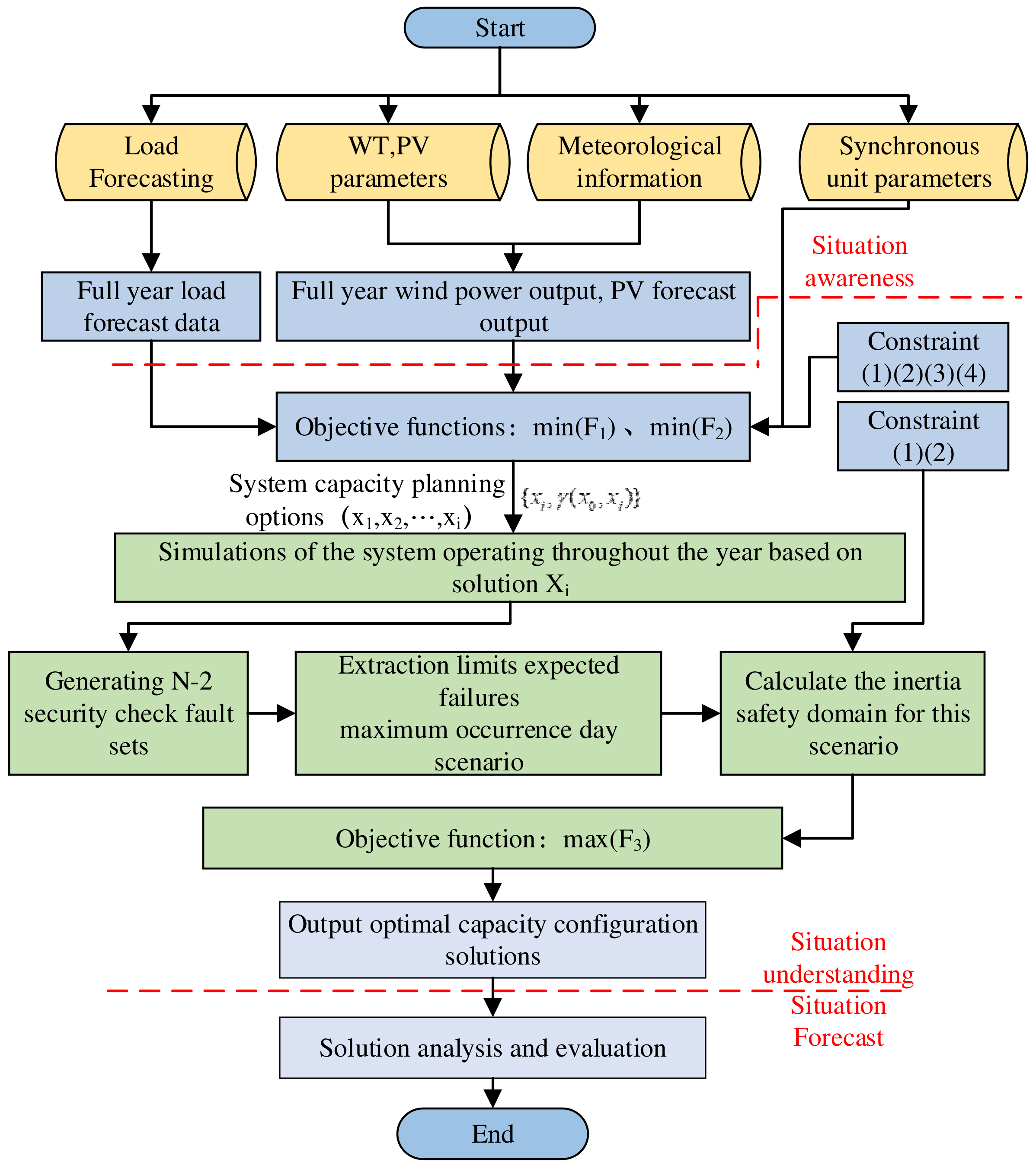
2.4. Situation Awareness Model for Capacity Planning of Wind-Photovoltaic-Thermal Power System

Applying the situation awareness approach to the planning of multiple power sources in the context of new power systems [13], the situation awareness-based capacity planning model is divided into four stages: situation awareness, situation understanding, situation prediction, and assisted decision-making [20]. Using situation awareness → situation understanding → situation prediction → assisted decision making → situation awareness to form a closed loop to fully grasp the system state and improve the accuracy of capacity allocation. The wind-photovoltaic-thermal power system capacity planning situation awareness model is shown in Figure 3.

(1)

Situation awareness: This is the stage of obtaining relevant data. This stage is mainly used to obtain equipment parameters, meteorological data, and user data in system power capacity planning through system measurement techniques, meteorological information prediction techniques, and load-side data prediction techniques.

(2)

Situation understanding: This is the stage of data analysis, which aims at understanding and mining the data obtained during the situation awareness stage, taking into account system stability, economy, environmental protection, etc., and analyzing the system operating dynamics of different capacity planning scenarios.

(3)

Posture prediction: This is the state prediction phase. For the capacity planning of multiple power systems, posture prediction is a comprehensive evaluation and analysis of different capacity planning options.

(4)

Assisted decision-making: Output the optimal solution, providing an effective basis for decision-making by relevant professionals.

3. Bi-Level Model for Optimal Capacity Allocation of Wind-Photovoltaic-Thermal Power Systems

3.1. Upper Level Model for Multi-Objective Optimal Configuration Considering the Environmental Friendliness and Economy of the System

The upper-level model is based on the objective of minimizing carbon emissions and total system cost over the whole life cycle of the system. The system capacity planning scheme is optimized based on the system power balance constraint, installed capacity constraint, generation unit output constraint, and thermal unit climbing constraint, and the decision variables are wind, PV, and thermal power output at each time.

3.1.1. Objective Functions

In this paper, the annual equivalent carbon emissions of wind power, photovoltaic power generation, and thermal power generation are calculated separately for the whole life cycle. The carbon emissions from wind, photovoltaic and thermal power plants are apportioned to the power generation process according to the carbon accounting model. The optimization objective is to minimize the annual carbon emissions of the wind-photovoltaic-thermal power system [21].

$$\begin{array}{l}\min F_1=\min \left\{{\displaystyle \sum _{\begin{array}{c}t=1\\ i\in N_{wind}\end{array}}^{8760}{P}_{wind,i}(t)R_{wind}{N}_{wind}{K}_{wind,i}}\right.+{\displaystyle \sum _{\begin{array}{c}t=1\\ j\in N_{pv}\end{array}}^{8760}{P}_{pv,j}(t)R_{pv}{N}_{pv}{K}_{pv,j}}\\ \left.\hspace{1em}\hspace{1em}\hspace{1em}\hspace{1em}\hspace{1em} +{\displaystyle \sum _{\begin{array}{c}t=1\\ k\in N_{SG}\end{array}}^{8760}{P}_{SG,k}(t)R_{SG}{N}_{SG}{K}_{SG,k}}\right\}\end{array}$$

(3)

where $R_{wind}$, $R_{pv}$, and $R_{SG}$ are the carbon emission factors of wind, photovoltaic and thermal power respectively for the whole life cycle of the system; $P_{wind,i}(t)$, $P_{pv,j}(t)$, $P_{SG,k}(t)$ represent the output power of the first wind turbine; $N_{wind}$, $N_{pv}$, and $N_{SG}$ are the number of wind turbines, photovoltaic cells, and synchronous machines respectively; $K_{wind,i}$, $K_{pv,j}$, and $K_{SG,k}$ are the switching states of wind turbines, photovoltaic cells, and synchronous units respectively.

Carbon emission factors can be calculated based on the Carbon Accounting Model [22,23].

Considering the economy, the total cost of the wind-photovoltaic-thermal power system consists of four parts: investment cost, operation cost, replacement cost, and maintenance cost. In this paper, only the operating costs of thermal power units are considered, and the operating costs of wind power and photovoltaic are approximated to be zero. The optimization objective is to minimize the total cost of the system.

$$\min F_2=\min \left\{P_{wind}+P_{pv}+P_{SG}\right\}$$

(4)

$$P_{wind}={\displaystyle \sum _{i=1}^{N_{wind}}(C_{wind,i}+\frac{C_{wind,r,i}}{{(1+r_1)}^{T_{wind,i}}}+{\displaystyle \sum _{t=1}^{Tt}\frac{C_{wind,m,i}}{{(1+r_1)}^t}})}$$

(5)

$$P_{pv}={\displaystyle \sum _{i=1}^{N_{pv}}(C_{pv,i}+\frac{C_{pv,r,1}}{{(1+r_2)}^{T_{pv}}}+{\displaystyle \sum _{t=1}^{Tt}\frac{C_{pv,m,i}}{{(1+r_2)}^t}})}$$

(6)

$$P_{SG}={\displaystyle \sum _{i=1}^{N_{SG}}(C_{SG,i}+\frac{C_{SG,r,i}}{{(1+r_3)}^{T_{SG}}}+{\displaystyle \sum _{t=1}^{Tt}\frac{C_{SG,m,i}}{{(1+r_3)}^t}}}+T_{SG}{\displaystyle \sum _{t=1}^{8760}\left[a_i{P}_{SG,i}{(t)}^2+b_i{P}_{SG,i}(t)+c_i\right]})$$

(7)

where $P_{wind}$, $P_{pv}$, and $P_{SG}$ are the total costs of wind, photovoltaic, and thermal power plants, respectively; $P_{SG,i}(t)$ is the output of thermal power unit i at time t; $C_{wind,i}$, $C_{pv,i}$, and $C_{SG,i}$ are the installed prices of a single wind turbine, a single photovoltaic cell unit, and a single synchronous machine, respectively; $N_{wind}$, $N_{pv}$, and $N_{SG}$ are the number of wind turbines, photovoltaic cells, and synchronous machines, respectively; $C_{wind,r,i}$, $C_{wind,m,i}$ are the replacement and maintenance costs of wind turbines, respectively; $C_{pv,r,i}$, $C_{pv,m,i}$ are the replacement and maintenance costs of photovoltaic cells, respectively; $C_{SG,r,i}$, $C_{SG,m,i}$ are the replacement and maintenance costs of thermal power units, respectively. The cost of replacement and maintenance of thermal units. The life cycle of the wind turbine, PV cell, and thermal unit, respectively; the project life and discount rate, respectively. The consumption characteristics of the thermal units are shown in $a_i$, $b_i$ and $c_i$ respectively.

3.1.2. Conditions of Constraint

(1)

Power balance constraints

Without considering the system network loss, the power generated by the system is equal to the power consumed by the load.

$$P_{LO}(t)={\displaystyle \sum _{i=1}^{N_{wind}}{P}_{wind,i}(t)K_{wind,i}}+{\displaystyle \sum _{j=1}^{N_{pv}}{P}_{pv,j}(t)K_{pv,j}}+{\displaystyle \sum _{k=1}^{N_{SG}}{P}_{SG,k}(t)K_{SG,k}}$$

(8)

where $P_{LO}(t)$ represents the power consumed by the load; $P_{wind,i}(t)$, $P_{pv,j}(t)$, and $P_{SG,k}(t)$ represents the output power of the i-th wind turbine, the j-th photovoltaic cell, and the k-th synchronous machine, respectively; $N_{wind}$, $N_{pv}$, and $N_{SG}$ is the number of wind turbines, photovoltaic cells, and synchronous machines, respectively; $K_{wind,i}$, $K_{pv,j}$, and $K_{SG,k}$ is the switching state of the wind turbine, photovoltaic cell, and synchronous unit, respectively.

(2)

Installed capacity constraint

Wind-photovoltaic-thermal power systems should have a certain amount of spare capacity, taking into account the possibility of failure of turbines, photovoltaics, synchronous machines, or unknown sudden increases in load in the system.

$${\displaystyle \sum _{i=1}^{N_{wind}}{P}_{wind,i}}+{\displaystyle \sum _{j=1}^{N_{pv}}{P}_{pv,j}}+{\displaystyle \sum _{k=1}^{N_{SG}}{P}_{SG,k}}\ge \lambda P_{LO,\max }$$

(9)

where $P_{wind,i}$, $P_{pv,j}$, and $P_{SG,k}$ represent the rated power of the i-th wind turbine, the j-th PV cell, and the k-th synchronous machine respectively; $P_{LO,\max }$ is the maximum load power; $\lambda$ is the load power factor.

(3)

Generator output constraints

The output of wind, photovoltaic and thermal power units should fluctuate within a certain range.

$$0\le P_{wind,i}(t)\le P_{wind,i,m}$$

(10)

$$0\le P_{pv,j}(t)\le P_{pv,j,m}$$

(11)

$$0\le P_{SG,k}(t)\le P_{SG,k,m}$$

(12)

where $P_{wind,i}(t)$, $P_{pv,j}(t)$, and $P_{SG,k}(t)$ represent the output power of the i-th wind turbine, the j-the photovoltaic cell, and the k-th synchronous machine respectively; $P_{wind,i,m}$, $P_{pv,j,m}$, and $P_{SG,k,m}$ represent the maximum output power of the wind turbine, the photovoltaic cell, and the synchronous machine respectively.

(4)

Climbing constraints for thermal power units

Thermal power units are required to meet a creep constraint, where the rate of change in power cannot exceed the creep rate during normal operation and can break the creep rate limit during start-up and shut-down.

$$-V_L{P}_{SG,i,m}\le P_{SG,i}(t)-P_{SG,i}(t-1)\le V_h{P}_{SG,i,m}$$

(13)

where $V_h$, $V_L$ are the maximum upward and downward climbing rates, respectively; $P_{SG,i,m}$ is the maximum output of thermal power unit i.

3.1.3. A Pareto Optimal Solution Set Decision Method Based on Grey Relativity Analysis

Grey relativity analysis (GRA) is a method of measuring the degree of association between factors based on the degree of similarity or dissimilarity of trends between them [24]. As the upper level optimization model is multi-objective optimization and it is difficult for the configuration solution to satisfy multiple objectives optimally at the same time [25]. The traditional method of using compromise weighting factors to transform into a single-objective function solution will inevitably affect the decision result of the configuration solution. To accurately evaluate the effect of multi-objective solution sets without destroying the integrity of the original solution set, this paper proposes a grey correlation method based on the Pareto optimal solution set evaluation method.

Firstly, GRA is used to calculate the correlation value between the Pareto optimal solution set and the ideal solution, and to establish a mapping between the Pareto optimal solution set and the correlation value to provide a basis for the lower level optimization model. The correlation value represents the degree of correlation between the solution set and the ideal solution. When evaluating the upper level model capacity configuration solution, the higher the correlation degree value, the greater the degree of correlation between the configuration solution and the ideal solution, and the better the configuration solution.

Assume that the set of optimal solutions of the upper level optimization model Pareto is $\left\{x_1,x_2,\dots ,x_n\right\}$, where $x_i=\{F_1,F_2\},i\in n$, $x_i$ denotes the set of objective values of configuration scheme i. Let the ideal solution $x_0=\left\{\min \right\{F_1\},\min \{F_2\left\}\right\}$, the correlation coefficient between the optimal solution set and the ideal solution can be solved using the GRA algorithm to construct the set of capacity configuration scheme-correlation mappings, $\{x_i,\gamma (x_0,x_i)\}$. $x_i$ is the capacity allocation solution i, $\gamma (x_0,x_i)$ is the correlation of $x_i$ based on the ideal solution, characterized as a label for the superiority or inferiority of solution $x_i$. The larger $\gamma (x_0,x_i)$, the better the solution.

3.2. Solving a Multi-Objective Configuration Upper Level Optimization Model for Systems Considering Environmental Friendliness and Economy

As the optimization upper-level optimization model is a multi-objective solution problem, the fast and elite mechanism of the non-dominated ranking multi-objective genetic algorithm (NSGA-II) has the advantages of efficiency and directness and is an effective method for solving multi-objective optimization problems [26].

The INSGA2-DS algorithm based on dominance strength uses (1) an improved fast sorting method based on dominance strength, (2) a novel distance algorithm that introduces the consideration of variance, and (3) a strategy of adaptive elite retention based on the NSGA-II algorithm. The improved algorithms can effectively improve the convergence and distribution problems of the NSGA-II algorithm. The introduction of the INSGA2-DS algorithm in this paper can effectively improve the distributivity and accuracy of the system capacity allocation scheme, avoid the flooding of good data, reduce the solution time, and improve the solution efficiency of the algorithm. Figure 4 shows the flow chart of the upper optimization model solution.

3.3. Optimal Configuration of the Lower Level Model Considering System Stability

To improve the frequency stability of the system, the upper model configuration scheme is further optimized based on the upper optimized model, taking into account the level of inertia margin of the system. The power system time-series operation simulation method [27] is introduced to simulate the time-series operation of all the planning solutions derived from the upper model in turn to find the inertia security region for each solution. The optimal capacity planning scheme is then optimized with the objective of combining the best system stability and economic and environmental characteristics. The optimization variables are the different capacity planning solutions output by the upper model.

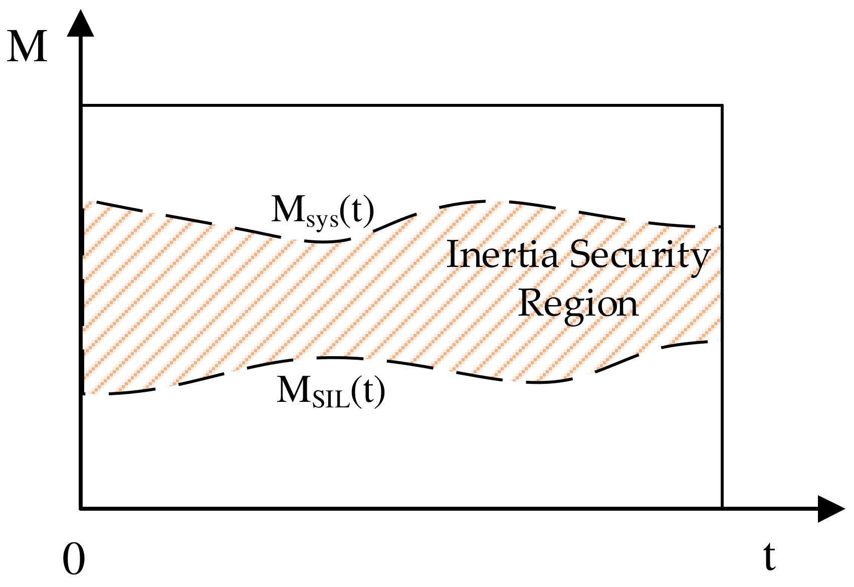
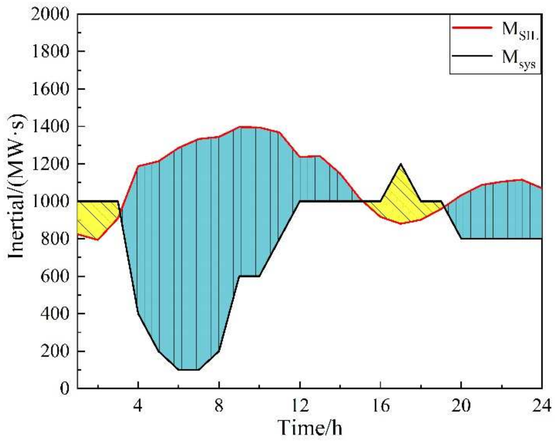
3.3.1. Inertia Security Region Model of the System

Inertia is the inherent ability of a power system to maintain frequency stability [28]. When the system is subjected to unpredictable power disturbances, frequency fluctuations occur within the system, when the rotational inertia present in the system helps to suppress rapid fluctuations in frequency and keep the frequency stable within a tolerable range [29,30]. Therefore, the inertia level of the system effectively reflects the frequency stability of the system.

According to the safety and stability standards proposed in the literature “Technical Guidelines for Safety and Stability Control of Power Systems”, the minimum inertia required to ensure system frequency stability under N-2 faults in power systems relying only on primary frequency regulation and second line of defense safety and stability control measures is the safety critical inertia value under this fault scenario. When the actual inertia of the system is less than the safe critical inertia, the occurrence of a serious fault within the system will trigger the system’s third line of defense safety device to act, and the system will be exposed to the risk of large area cut-off and load shedding. In this paper, the inertia value corresponding to the most severe failure scenario in the N-2 safety calibration of the system in the operating scenario is defined as the system safety critical inertia value $M_{SIL}$ [6].

$$M_{SIL}=\max \{M_{SIL,F_{12}},\dots ,M_{SIL,F_{ij}}\}$$

(14)

where $M_{SIL,F_{ij}}$ is the safety critical inertia corresponding to the failure of component i, j; $i\ne j$ and $i,j\le N_t$; $N_t=N_{SG}+N_w+N_p$; $N_t$ is the total number of components; $N_{SG}$ is the number of thermal power plants; $N_w$ is the number of wind farms; $N_p$ is the number of photovoltaic plants.

To quantify the system inertia level, the relative magnitude of the actual system inertia value to the safety critical system inertia value is defined as the system inertia margin.

$$K_m=\frac{M_{sys}-M_{SIL}}{M_{SIL}}\times 100\%$$

(15)

where $K_m$ is the system inertia margin; $M_{sys}$ is the actual system inertia value; $M_{SIL}$ is the system safety critical inertia value $K_m$ is the system inertia margin at a certain time. According to the operating characteristics of the power system, the system inertia margin varies at different times and is not continuous. The system Inertia security region is shown in Figure 5.

Considering continuous operation periods, define the inertia security region of the system, which is the area of the system inertia margin over a length of time T.

$$K_M={\displaystyle {\int }_0^T\left[M_{sys}(t)-M_{SIL}(t)\right]}dt$$

(16)

where $M_{sys}(t)$, $M_{SIL}(t)$ are the actual inertia and the safety critical inertia of the system at time t, respectively, and T is the length of time.

When the system inertia is the inertia security region, the system inertia can mitigate sudden changes in frequency caused by a potentially large disturbance fault in the system, avoiding large cuts in the system and load shedding.

In order to improve the calculation efficiency of the model, the rotational inertia of the system is considered in this paper. The rotational inertia of the turbine is ignored because the rotational kinetic energy provided by the turbine is related to the operating conditions, there are more variable factors, and it has less influence on the inertia of the system. Therefore, only the rotational inertia provided by the thermal power unit is considered.

The formula for calculating the actual inertia of the system:

$$M_{sys}={\displaystyle \sum _{i=1}^{N_{SG}}{H}_i{P}_i{K}_i}$$

(17)

where $M_{sys}$ is the actual inertia value of the generation system; $H_i$ is the time constant of inertia of the thermal unit i; $P_i$ is the rated power of the thermal unit i; $K_i$ is the switching state of the thermal unit. When the thermal unit is on, $K_i=1$, and when it is off, $K_i=0$.

In the case of a power generation system, the actual inertia value of the system can be solved using the system operating scenario for the thermal power unit and its parameters.

The following equation for calculating the safe critical inertia value of the system is derived. Typically, when active disturbances occur in the system, ignoring damping effects, the equation of motion for the system equivalent rotor is:

$$2\frac{M_{\mathrm{sys}}}{f_N}\frac{df(t)}{dt}=P_m(t)-P_e(t)$$

(18)

where $f_N$ is the nominal frequency; $P_m(t)$ is the total mechanical power of the system at time t; $P_e(t)$ is the total electromagnetic power of the system at time t; $f(t)$ is the system frequency at time t.

In the event of an active disturbance in the system, $\left|RoCoF\right|$ reaches a maximum at the moment of the disturbance $t_{0+}$ because frequency control measures act immediately to reduce the unbalanced power:

$$RoCoF(t_{0+})=-\frac{f_N\Delta P}{2(M_{SIL}-M_{loss})}$$

(19)

where $RoCoF(t_{0+})$ is the rate of change of system frequency for the most severe fault in the system N-2 safety calibration fault set; $f_N$ is the nominal frequency; $\Delta P$ is the active power disturbance from the limit expected fault; and $M_{loss}$ is the loss of inertia due to the limit expected fault.

According to Equations (18) and (19), the system safety critical inertia is obtained:

$$M_{SIL}=\max \left\{\begin{array}{c}{M}_{loss}-\frac{f_N\Delta P}{2RoCo{F}_{\min }} , \Delta P>0\\ M_{loss}-\frac{f_N\Delta P}{2RoCo{F}_{\max }} , \Delta P<0\end{array}\right.$$

(20)

where $RoCo{F}_{\max }$ is the upper limit of the rate of change of the system frequency; $RoCo{F}_{\min }$ is the lower limit of the rate of change of the system frequency.

3.3.2. Objective Functions

To measure the degree of economy and environmental friendliness of the capacity allocation scheme of the upper level optimization model, a correlation factor ${\mu }_i$ is proposed. The correlation factor is calculated as:

$${\mu }_i=\frac{{\gamma }_i}{\overline{\gamma }}$$

(21)

$$0<{\gamma }_i\le 1$$

(22)

where ${\gamma }_i$ is the correlation of option $x_i$; $\overline{\gamma }$ is the average of the correlation of all options ${\gamma }_i$ characterizes the combined economic and environmental performance of option $x_i$. The larger ${\gamma }_i$ is, the greater the correlation between option $x_i$ and the ideal option, and the better the combined level of economy and environmental friendliness.

The correlation factor ${\mu }_i$ measures the degree of economy and environmental friendliness of the upper model capacity configuration. It is known that $K_M$ is the system inertia security region. Obviously, the larger the system inertia safety domain is, the more beneficial to system stability. In order to improve the efficiency of the solution and make the decision scheme informative, the scenario of the maximum occurrence of the system limit expected failure day in one year is selected as a typical day, and the inertia safety domain of the typical day $K_{M1}$ is defined:

$$K_{M1}={\displaystyle {\int }_0^{24}\left[M_{sys,i}(t)-M_{SIL,i}(t)\right]}dt$$

(23)

where $M_{sys,i}(t)$ is the actual inertia of the system at time t for scenario $x_i$ on a typical day; $M_{SIL,i}(t)$ is the critical inertia of the system at time t for scenario $x_i$ on a typical day; and ${\mu }_i$ is the correlation factor for scenario $x_i$.

Based on the configuration scheme of the upper level optimization model, the objective function is established by considering the economy, environmental protection, and stability of the system:

$$\max F_3=\max \left\{{\mu }_i{K}_{M1}\right\}$$

(24)

3.3.3. Conditions of Constraint

(1)

System inertia and rate of change of frequency constraints

The inertia and rate of change of frequency of the system shall be maintained within a range of:

$$M_{\min }\le M_{SIL}\le M_{\max }$$

(25)

$$M_{sys}(t)\ge M_{SIL}(t)$$

(26)

where $M_{\max }$ and $M_{\min }$ are the upper and lower limits of the system inertia, respectively.

(2)

System frequency rate of change constraint

$$RoCo{F}_{\min }\le RoCoF\le RoCo{F}_{\max }$$

(27)

where $RoCo{F}_{\max }$ and $RoCo{F}_{\min }$ are the upper and lower limits of the rate of change of the system frequency, respectively.

4. Bi-Level Model Solving for Optimal System Capacity Allocation

For system planning, the lack of actual output parameters for wind farms and photovoltaic power stations makes it difficult to perform direct calculations, so historical average meteorological data are used for output forecasting.

For the upper level model, the local historical average meteorological data information is combined with the predicted new energy output data based on the wind turbine and PV unit parameters, and the load data is predicted. As the upper optimization model is a multi-objective problem, INSGA2-DS is used to solve the algorithm and output the Pareto solution set for the upper model capacity configuration, and the Pareto optimal solution set evaluation method based on GRA is used to obtain the solution-correlation mapping set $\{x_i,\gamma (x_0,x_i)\}$ as input to the lower optimization model.

For the lower level model, first determine the various types of boundary conditions, introduce the power system time-series operation simulation method of literature [27], carry out year-round operation simulation based on the capacity configuration scheme of the upper level model, and then combine the system stability control strategy to generate N-2 safety check fault sets. Then, extract the system limit expected fault maximum occurrence day scenario, and solve the lower level optimization model [31,32].

Table 1. Bi-level model for optimal system capacity planning.

Project	Upper Optimization Model	Lower Optimization Model
Decision variables	Wind, PV and thermal power output	Upper model solving solutions
Conditions of constraint	(1)(2)(3)(4)	(5)(6)
Objective functions	minF1, minF2	max F3
Solution algorithms	INSGA2-DS	Cplex solvers
Optimization objectives	Minimal carbon emission and lowest total cost	Combination of economy, environmental friendliness, and stability

shows a Bi-level model for optimal system capacity planning. Figure 6 shows the framework for optimal capacity allocation of wind-photovoltaic-thermal power systems.

5. Case Study

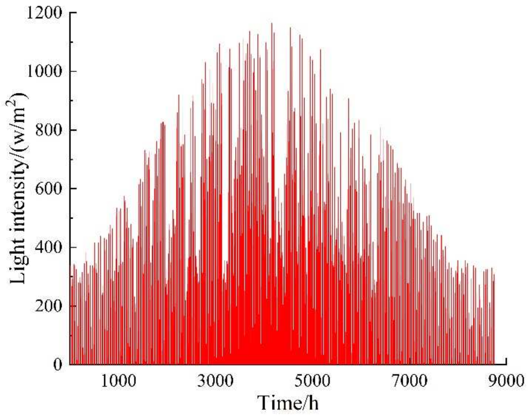
5.1. Date Preprocessing

This paper uses a method for simulating the time-series operation of power systems based on meteorological data, as the planned wind-light-fire system lacks actual output data and is difficult to apply directly in simulation tools.

Based on the local average historical meteorological data information and historical load data for a region of the country, predictions are made including annual wind speed, temperature, light intensity, and annual load data, as shown in Figure 7, Figure 8, Figure 9 and Figure 10. Suitable wind turbine, PV cell, and thermal power unit parameters are selected based on the load demand and meteorological data. The carbon emission factor parameters for the full life cycle of the system are shown in

Table A1. Thermal power unit parameters.

Parameters	Number
Power rating/MW	40
Maximum power/MW	40
Minimum power/MW	10
a/(¥/MWh)	0.024
b/(¥/MWh)	78
c/¥	960
Inertia time constant/s	5
R/(kg/kWh)	0.95

,

Table A2. Wind turbine parameters.

Parameters	Number
Power rating/MW	1.5
Cut-in wind speed Vin/(m/s)	3
Rated wind speed Vn/(m/s)	10
Cut-out wind speed Vout/(m/s)	30
R/(kg/kWh)	0.012

and

Table A3. Photovoltaic cell parameters.

Parameters	Number
Ps/(kWh)	0.2
Gs/lx	1000
γ/(%/°C)	−0.5
Tτ/°C	25
R/(kg/kWh)	0.035

in Appendix A. The cost and life cycle of each part of the system are shown in

Table A4. System component costs and life cycle.

Parameters	Thermal Power Units	Wind Turbines	Photovoltaic Cells
Investment cost/(¥)	1.125 × 108	1.097 × 107	1242
Replacement cost/(¥)	1.125 × 108	1.097 × 107	1242
Maintenance cost/(¥/yr)	1.125 × 106	1.097 × 105	12.42
Life cycle/(yr)	15	20	30

in Appendix A. The INSGA2-DS algorithm was set to 100 iterations and run 10 times to obtain stable results for the algorithm. The Pareto optimal solution set for 60 sets of capacity allocation scenarios was obtained after the upper level model optimization solution, and the scenario-correlation mapping set was established and imported into the lower level optimization model for the solution.

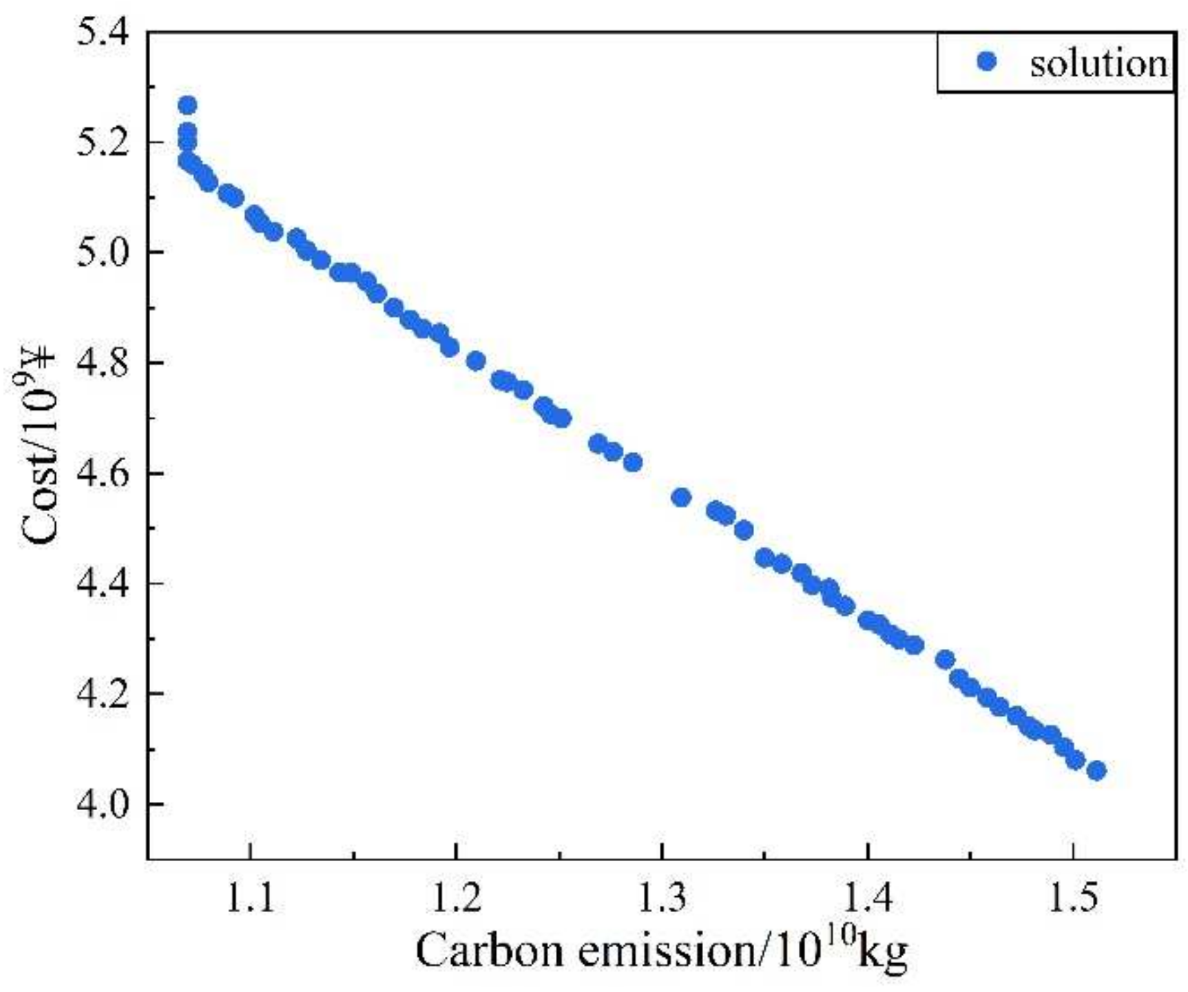
5.2. Optimal Capacity Configuration Solution

The upper model is solved using the INSGA2-DS algorithm and the lower model is solved using the MATLAB software solver.

Table 2. Optimal capacity configuration solution.

Configuration Solutions	Number
Number of WT	51
Number of PV cells	104,354
Number of thermal power units	8
Costs/¥	4.95 × 109
Carbon emission/kg	1.16 × 1010
Inertia security region/MW·s2	10,308.2
Correlation factor	1.38
Installed capacity of thermal power generation/MW	320
Installed capacity of wind power/MW	76.5
Installed capacity of photovoltaic power/MW	20.9

shows the optimal capacity configuration of the wind–photovoltaic–thermal power system that meets the requirements. Figure 11 shows the set of Pareto scenarios for the capacity configuration of the upper model.

To verify the rationality of the optimal capacity allocation scheme, three different schemes are arbitrarily selected from the output scheme class of the upper optimization model for comparison and analysis. Option 1 is the optimal capacity allocation solution.

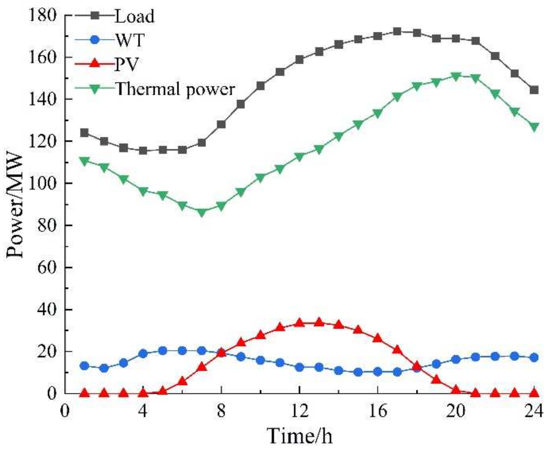
5.3. Simulation Analysis of the Timing Operation of Different Planning Scenarios

This paper uses a modified IEEE-39 node system as a research case. Figure 12 shows the modified IEEE-39 node network topology.

The IEEE-39 node arithmetic example is built on the MATLAB platform, with 1–8 connected to synchronous machines, 9 to an equivalent wind farm, and 10 to an equivalent PV plant. As the single generator output accounts for a relatively high total load, each limit expected fault type is either a synchronous unit tripping or a new energy field station going off-grid. The scenario of the maximum occurrence day of the limit scenario fault is selected for analysis. $R_{\max }$ and $R_{\min }$ are 2 Hz/s and −2 Hz/s respectively.

Scenario 1 is the optimal capacity allocation solution derived from the lower level model. During a typical day, 6 thermal units are expected to be on at moments 1–10; 8 thermal units are expected to be on at the remaining moments. As can be seen from Figure 13, during periods 1–3 and 12–24 on a typical day, the wind power output is less than the rated power because the actual wind speed is lower than the rated wind speed of the wind turbine, and the photovoltaic units can only generate power during the day, making it necessary for the thermal units to increase their power output to meet the power demand at the load side while satisfying the boundary conditions. During the 4–9 period, the wind power output reaches its maximum, and due to the low load demand at this time, the thermal power units must reduce their output by reducing the number of units on in order to reduce wind and light abandonment.

As can be seen from Figure 14, the moment of occurrence of the limit fault of the system in Scenario 1 is t = 5–9, the actual inertia of the system at all times during a typical day is greater than the value of the system safety critical inertia, and the inertia margins are all positive. The inertia of the system under the limit expected fault is sufficient to support the frequency fluctuation, which can effectively reduce the risk of a major outage accident.

The typical daily inertia security region for scenario 1 is K_M1 = 10,308.2 MW·s², ${\mu }_i$ = 1.38 and F₃ = 14,225.316 MW·s². As the system operating state varies with time, the system limit failure varies from moment to moment, exhibiting the time-varying nature of the system safety critical inertia values. When t = 3, t = 4, and t = 10, the system corresponds to a smaller limit expected failure with a smaller inertia requirement, when the system inertia is more abundant. In contrast, when t = 5–9, the actual inertia of the system is close to the system’s safe critical inertia, and the system is at a low inertia level at this time.

Scenario 2 is the capacity allocation option with the largest correlation factor, and the specific capacity allocation can be seen in

Table 3. Different capacity configuration solutions.

Solution Configuration	Scenario 1	Scenario 2	Scenario 3	Scenario 4
Number of WT	51	71	15	74
Number of PV cells	104,354	104,525	103,790	104,739
Number of thermal power units	8	7	9	7

.

As can be seen in Figure 15, Scenario 2 has a different share of wind, PV and thermal power output due to the different number of installed thermal, wind and PV units compared to Scenario 1. In the periods 2–12 and 20–24 on a typical day, wind power output is higher due to the higher installed capacity of the turbines. Especially in the 3–12 period, wind power output is much higher than thermal power output. At this time, the number of thermal units must be reduced to meet the load demand.

As can be seen in Figure 16, the typical daily inertia security region for scenario 2 is K_M1 = −8614.6 MW·s², ${\mu }_i$ = 1.55, F₃ = −13,352.63 MW·s².At moments 3–14 and 19–24, the actual system inertia is lower than the system safety critical inertia value, with the system inertia deficit reaching a maximum of 1233 MW·s at moment 7, when the system faces a very high risk of frequency destabilization. This is due to the low thermal power output and the high proportion of new energy sources. When a major fault occurs in the system, such as a new energy source going off-grid, the system frequency will be destabilized due to the lack of sufficient inertia support, which will result in a large-scale power outage. The length of time that the actual inertia of the system is below the system safety critical inertia value is 517 h throughout a year.

Scenario 3 is the least costly option to consider, with a typical daily inertia security region of K_M1 = 16,802 MW·s², ${\mu }_i$ = 0.74, and F₃ = 12,433.48 MW·s². As can be seen from Figure 17, the system has a higher share of thermal power output and a smaller peak-to-valley differential. In the period 8–17, the combined share of wind and PV output is higher, peaking at around 26%. Figure 18 shows a typical daily inertia security region for Scenario 3.

Scenario 4 is the case where carbon emissions are considered to be minimal. As shown in Figure 19, the typical daily output characteristics of scenario 4 are similar to those of scenario 2 due to the similarity between the capacity configuration scheme of scenario 2 and that of scenario 4. The typical daily inertia security region K_M1 = −8871.2 MW·s², ${\mu }_i$ = 1.49, and F₃ = −13,218.09 MW·s². The length of time during a year when the actual system inertia is below the system safety critical inertia value is greater than in Scenario 2, amounting to 780 h. Figure 20 shows a typical daily inertia security region for Scenario 4.

In summary, the system is able to ensure continuous and stable power supply on a typical day for all capacity configuration options, subject to constraints, such as meeting load demand and weather forecast data.

5.4. Comprehensive Characterisation of Different Configuration Scenarios

A comprehensive analysis of the economy, environmental friendliness, and stability of the four scenarios.

As can be seen from Figure 21, the inertia security region for scenarios 2 and 4 is negative, which is because the new energy output is higher during a typical day and the thermal units are in a lower output state, resulting in the actual inertia level of the system is lower than the system safety critical inertia value, and therefore scenarios 2 and 4 have a frequency stability risk. As the typical day is the maximum day scenario of the yearly limit expected fault occurrence, the inertia security region of scenarios 1 and 3 are 10,308.2 MW·s² and 16,802 MW·s² respectively, so there are no negative inertia margin operation scenarios for scenarios 1 and 3 during the yearly operation.

The economic analysis of different scenarios shows that scenario 3 has the lowest total cost, which is because the unit price of new energy is higher than that of thermal units per unit of capacity, while scenario 3 has the smallest total amount of new energy installed and the system generation output is mainly borne by thermal units, thus the total cost of scenario 3 is low. In addition, scenario 1 also has a lower total cost of CNY 4.951 × 10⁹, which is 4.18% and 6% lower than scenarios 2 and 4 respectively.

For the carbon emissions analysis, the carbon emissions from electricity generation are smaller for scenarios 2 and 4 due to their larger installed new energy capacity. The difference in carbon emissions between scenarios 1, 2, and 4 is not significant, within 7%. As the installed capacity of thermal power units is higher and the installed capacity of new energy is lower, the carbon emissions from scenario 3 are the largest, with scenario 1 emitting 3.514 × 10⁹ kg less carbon than scenario 3, or approximately 23.25%.

An analysis of the characteristics of the different options shows that as the correlation factor increases, the carbon emissions of the system gradually decrease, while the total cost does not change much. Therefore, the correlation factor can be used to effectively evaluate the merits of the capacity allocation options. Scenario 2, with the highest correlation factor, is the best capacity allocation option if the system stability is not considered and only the system economy and environmental protection are taken into account. However, the actual inertia of the system will be lower than the safety critical inertia of the system during the operation of scenario 2, which will lead to low frequency load shedding or high cycle cut-off of the grid in case of serious failure. Therefore, the capacity configuration of scenario 2 requires an appropriate increase in the number of synchronous machines to increase the inertia of the system, while the number of turbines and PV units should be reduced to reduce wind and light abandonment and to enhance the economy of the system.

In summary, scenario 1 takes into account system economy, environmental friendliness, and stability. Scenario 1 can therefore be used as the best capacity configuration for the system.

5.5. Impact of Optimization Algorithms on Capacity Planning

To verify the superiority of INSGA2-DS in solving capacity planning problems, the NSGA-II algorithm was used for comparative analysis. As shown in Figure 22, the Pareto frontier solution is more widely distributed and can effectively avoid getting trapped in a local optimum.

A comparison of the operational characteristics of the two algorithms is shown in

Table 4. Comparison of NSGA-II and INSGA2-DS characteristics.

Algorithms	Population Size/Unit	Number of Convergence Iterations/Time	Calculation Efficiency/s
NSGA-II	300	120	101
INSGA2-DS	300	100	84

. For the same number of populations, INSGA2-DS has a shorter computation time than NSGA-II and converges at a faster rate, with a computational efficiency improvement of about 17%. Therefore, INSGA2-DS is more suitable for the problem of capacity optimization allocation of wind-light-fire systems.

6. Conclusions

This paper proposes a situation awareness-based capacity optimization strategy for wind–photovoltaic–thermal power systems. A bi-level model is established for the optimal allocation of system capacity. The upper model takes into account the carbon emissions and total system cost of the whole life cycle of the system and ensures the effectiveness and practicality of the upper model through the system power balance constraint, installed capacity constraint, generator output constraint, and thermal unit climbing constraint. The Pareto-based capacity allocation scheme is solved using the INSGA2-DS algorithm, and the Pareto optimal solution set evaluation method based on GRA is used to establish the scheme-relation degree mapping set, which is used as the input of the lower model. The lower model integrates the maximum inertia security region of the system, the best economy, and environmental protection as the optimization objectives to optimize the capacity allocation scheme. Finally, the effectiveness of the proposed strategy and algorithm is verified by means of an arithmetic example.

This provides new practical ideas and methods for planning the capacity allocation of wind–photovoltaic–thermal power systems in the context of new power systems, and is a guide to the problem of planning the capacity of power sources in the context of the new power system. The wind–photovoltaic–thermal power system capacity optimization model developed in this paper can ensure the best system stability and minimize carbon emissions and total costs within a certain range.

The method proposed in the paper focuses on three forms of power sources, namely wind, light, and fire, and will be followed by subsequent studies to include multi-energy matching of systems, such as hydropower and energy storage.

References

1. Bistline, J.E.T.; Brown, M.; Siddiqui, S.A.; Vaillancourt, K. Electric sector impacts of renewable policy coordination: A multi-model study of the North American energy system. Energy Policy 2020, 145, 111707. [Google Scholar] [CrossRef]
2. Helisto, N.; Kiviluoma, J.; Holttinen, H.; Lara, J.D.; Hodge, B.-M. Including operational aspects in the planning of power systems with large amounts of variable generation: A review of modeling approaches. Wiley Interdiscip. Rev.-Energy Environ. 2019, 8, 341. [Google Scholar] [CrossRef]
3. Xu, Y.; Tu, J.; Yin, Z. The capacity selection of wind photovoltaic power generations based on KELM method. Electr. Meas. Instrum. 2019, 56, 73–80. [Google Scholar]
4. Tang, H.; Yang, G.; Wang, P.; Li, Q.; Zhang, L.; Liu, S.; Qin, J. Capacity Optimal Configuration of Wind/PV Hybrid Power System Based on Carbon Dioxide Emission. Electr. Power Constr. 2017, 38, 108–114. [Google Scholar]
5. Xu, Y.; Lang, Y.; Wen, B.; Yang, X. An Innovative Planning Method for the Optimal Capacity Allocation of a Hybrid Wind-PV-Pumped Storage Power System. Energies 2019, 12, 2809. [Google Scholar] [CrossRef] [Green Version]
6. Liu, J.; He, D. Profit Allocation of Hybrid Power System Planning in Energy Internet: A Cooperative Game Study. Sustainability 2018, 10, 388. [Google Scholar] [CrossRef] [Green Version]
7. Ye, C.-J.; Liu, W.-D.; Fu, X.-H.; Wang, L.; Huang, M.-X. Capacity allocation of hybrid solar-wind energy system based on discrete probabilistic method. Turk. J. Electr. Eng. 2015, 23, 1913–1929. [Google Scholar] [CrossRef]
8. Xu, M.; Zhuan, X. Optimal planning for wind power capacity in an electric power system. Renew. Energy 2013, 53, 280–286. [Google Scholar] [CrossRef]
9. Emmanuel, M.; Doubleday, K.; Cakir, B.; Markovic, M.; Hodge, B.-M. A review of power system planning and operational models for flexibility assessment in high solar energy penetration scenarios. Sol. Energy 2020, 210, 169–180. [Google Scholar] [CrossRef]
10. Dhaliwal, N.K.; Bouffard, F.; O’Malley, M.J. A Fast Flexibility-Driven Generation Portfolio Planning Method for Sustainable Power Systems. IEEE Trans. Sustain. Energy 2021, 12, 368–377. [Google Scholar] [CrossRef]
11. Lin, X.; Wen, Y.; Yang, W. Inertia Security Region: Concept, Characteristics, and Assessment Method. Proc. CSEE 2021, 41, 3065–3079. [Google Scholar]
12. Wen, Y.; Lin, X. Minimum Inertia Requirement Assessment of Microgrids in Islanded and Grid-connected Modes. Proc. CSEE 2021, 41, 2040–2053. [Google Scholar]
13. Basu, C.; Padmanaban, M.; Guillon, S.; Cauchon, L.; De Montigny, M.; Kamwa, I. Situational awareness for the electrical power grid. IBM J. Res. Dev. 2016, 60, 7384562. [Google Scholar] [CrossRef]
14. Yang, J.; Zhang, P.; Xu, X.; Xu, T. Research Status of Power Grid Situation Awareness Technology in China and Abroad. East China Electr. Power. 2013, 41, 1575–1581. [Google Scholar]
15. Ge, L.; Li, Y.; Chen, Y. Key Technologies of Situation Awareness and Implementation Effectiveness Evaluation in Smart Distribution Network. High Volt. Eng. 2021, 47, 2269–2280. [Google Scholar]
16. Oree, V.; Hassen, S.Z.S.; Fleming, P.J. Generation expansion planning optimisation with renewable energy integration: A review. Renew. Sustain. Energy Rev. 2017, 69, 790–803. [Google Scholar] [CrossRef]
17. Wang, Z.; Shi, Y.; Tang, Y.; Men, X.; Cao, J.; Wang, H. Low Carbon Economy Operation and Energy Efficiency Analysis of Integrated Energy Systems Considering LCA Energy Chain and Carbon Trading Mechanism. Proc. CSEE 2019, 39, 1614–1626. [Google Scholar]
18. Ardente, F.; Beccali, M.; Cellura, M.; Lo Brano, V. Energy performances and life cycle assessment of an Italian wind farm. Renew. Sustain. Energy Rev. 2008, 12, 200–217. [Google Scholar] [CrossRef]
19. Luo, W.; Khoo, Y.S.; Kumar, A.; Low, J.S.C.; Li, Y.; Tan, Y.S.; Wang, Y.; Aberle, A.G.; Ramakrishna, S. A comparative life-cycle assessment of photovoltaic electricity generation in Singapore by multicrystalline silicon technologies. Sol. Energy Mater. Sol. Cells 2018, 174, 157–162. [Google Scholar] [CrossRef]
20. Oladeji, I.; Zamora, R.; Lie, T.T. An online security prediction and control framework for modern power grids. Energies 2021, 14, 6639. [Google Scholar] [CrossRef]
21. Yang, B.; Guo, Y.; Xiao, X.; Tian, P. Bi-level Capacity Planning of Wind-PV-Battery Hybrid Generation System Considering Return on Investment. Energies 2020, 13, 3046. [Google Scholar] [CrossRef]
22. Kumar, I.; Tyner, W.E.; Sinha, K.C. Input-output life cycle environmental assessment of greenhouse gas emissions from utility scale wind energy in the United States. Energy Policy 2016, 89, 294–301. [Google Scholar] [CrossRef]
23. Kadiyala, A.; Kommalapati, R.; Huque, Z. Characterization of the life cycle greenhouse gas emissions from wind electricity generation systems. Int. J. Energy Environ. Eng. 2017, 8, 55–64. [Google Scholar] [CrossRef] [Green Version]
24. Li, C.; Zhao, G.; Meng, J.; Zheng, Z.; Yu, S. Multi-Objective Optimization Strategy Based on Entropy Weight, Grey Correlation Theory, and Response Surface Method in Turning. Int. J. Ind. Eng.-Theory 2021, 28, 490–507. [Google Scholar]
25. Tan, Y.-Y.; Jiao, Y.-C.; Li, H.; Wang, X.-K. A modification to MOEA/D-DE for multiobjective optimization problems with complicated Pareto sets. Inf. Sci. 2012, 213, 14–38. [Google Scholar] [CrossRef]
26. Verma, S.; Pant, M.; Snasel, V. A Comprehensive Review on NSGA-II for Multi-Objective Combinatorial Optimization Problems. IEEE Access 2021, 9, 57757–57791. [Google Scholar] [CrossRef]
27. Liu, X.; Lu, X.; Lou, Y.; Zhao, Y.; Wei, L.; Zhao, W. Optimal setting of wind-thermal-bundled capacity ratio based on chronological operation simulation. Power Syst. Prot. Control 2021, 49, 53–62. [Google Scholar]
28. Rezkalla, M.; Pertl, M.; Marinelli, M. Electric power system inertia: Requirements, challenges and solutions. Electr. Eng. 2018, 100, 2677–2693. [Google Scholar] [CrossRef] [Green Version]
29. Gu, H.; Yan, R.; Saha, T.K.; Muljadi, E. System Strength and Inertia Constrained Optimal Generator Dispatch under High Renewable Penetration. IEEE Trans. Sustain. Energy 2020, 11, 2392–2406. [Google Scholar] [CrossRef]
30. Wang, B.; Yang, D.; Cai, G. Review of Research on Power System Inertia Related Issues in the Context of High Penetration of Renewable Power Generation. Power Syst. Technol. 2020, 44, 2998–3007. [Google Scholar]
31. Wang, J.; Dong, F.; Ma, Z.; Chen, H.; Yan, R.; Klemes, J.J. Multi-objective optimization with thermodynamic analysis of an integrated energy system based on biomass and solar energies. J. Clean. Prod. 2021, 324, 129257. [Google Scholar] [CrossRef]
32. Li, J.; Xu, W.; Cui, P.; Qiao, B.; Feng, X.; Xue, H.; Wang, X.; Xiao, L. Optimization configuration of regional integrated energy system based on standard module. Energy Build. 2020, 229, 110485. [Google Scholar] [CrossRef]
Figure 1. Wind-photovoltaic-thermal power system characteristics.
Energies 15 03298 g001
Figure 2. Trends in carbon emissions, rotational inertia, and proportion of thermal power.
Energies 15 03298 g002
Figure 3. Situation awareness model for capacity planning of wind-photovoltaic-thermal power systems.
Energies 15 03298 g003
Figure 4. Flow chart of the upper optimization model solution.
Energies 15 03298 g004
Figure 5. Inertia security region of the system.
Energies 15 03298 g005
Figure 6. Framework for optimal capacity allocation of wind-photovoltaic-thermal power systems.
Energies 15 03298 g006
Figure 7. Full year wind speed forecast curve.
Energies 15 03298 g007
Figure 8. Full year temperature forecast curve.
Energies 15 03298 g008
Figure 9. Full year light intensity prediction curve.
Energies 15 03298 g009
Figure 10. Full year load forecast curve.
Energies 15 03298 g010
Figure 11. Pareto frontage diagram.
Energies 15 03298 g011
Figure 12. Modified IEEE-39 node network topology.
Energies 15 03298 g012
Figure 13. Typical daily power curve for scenario 1.
Energies 15 03298 g013
Figure 14. Typical daily inertia security region for scenario 1.
Energies 15 03298 g014
Figure 15. Typical daily power curve for scenario 2.
Energies 15 03298 g015
Figure 16. Typical daily inertia security region for scenario 2.
Energies 15 03298 g016
Figure 17. Typical daily power curve for scenario 3.
Energies 15 03298 g017
Figure 18. Typical daily inertia security region for scenario 3.
Energies 15 03298 g018
Figure 19. Typical daily power curve for scenario 4.
Energies 15 03298 g019
Figure 20. Typical daily inertia security region for scenario 4.
Energies 15 03298 g020
Figure 21. Characteristics of different scenarios.
Energies 15 03298 g021
Figure 22. NSGA-II and INSGA2-DS optimization results.
Energies 15 03298 g022