Article

Three-Dimensional Numerical Characterization of High-Temperature Superconductor Bulks Subjected to Rotating Magnetic Fields

1
Faculty of Engineering and IT, University of Technology Sydney, Sydney, NSW 2007, Australia
2
School of Electrical and Information Engineering, University of Sydney, Sydney, NSW 2006, Australia
3
School of Electrical and Information Engineering, Tianjin University, Tianjin 300072, China
4
Electrical Engineering Division, University of Cambridge, Cambridge CB3 0FA, UK
*
Authors to whom correspondence should be addressed.
Energies 2022, 15(9), 3186; https://doi.org/10.3390/en15093186
Submission received: 23 March 2022 / Revised: 17 April 2022 / Accepted: 25 April 2022 / Published: 27 April 2022
(This article belongs to the Special Issue New Advances in Permanent Magnet Electrical Machines)

Abstract

:
High-temperature superconductor (HTS) bulks have shown very promising potential for industrial applications due to the ability to trap much higher magnetic fields compared to traditional permanent magnets. In rotating electrical machines, the magnetic field is a combination of alternating and rotating fields. On the contrary, all studies on electromagnetic characterization of HTS presented in the literature so far have only focused on alternating AC magnetic fields and alternating AC loss due to the unavailability of robust experimental techniques and analytical models. This paper presents a numerical investigation on the characterization of HTS bulks subjected to rotating magnetic fields showing AC loss, current density distribution in three-dimensional axes, and trapped field analysis. A three-dimensional numerical model has been developed using H-formulation based on finite element analysis. An HTS cubic sample is magnetized and demagnetized with two-dimensional magnetic flux density vectors rotating in circular orientation around the XOY, XOZ, and YOZ planes.

1. Introduction

Over three decades, high-temperature superconductors have shown promising capabilities and possibilities for high-performance large-scale electrical machines [1]. HTS bulks fabricated from RE–Ba–Cu–O (RE stands for rare-earth element) by top-seeded melt growth technique have the ability to trap much higher magnetic fields at low temperatures, unlike traditional permanent magnets. The magnetic field strength trapped in HTS permanent magnets can be significantly increased with the sample size and value of critical current density. Currently, HTS magnets hold the world record of 17.9 T of the trapped magnetic field [2]. This distinctive property makes these trapped field magnets suitable candidates for designing compact, lightweight, and energy-efficient electrical machines having outstanding high-power densities [3,4] ranging from high-performance electrical motors [5] to HTS magnetic levitation [6]. Besides their applications in electrical machines, there have been significant advancements in superconducting electronics such as antennae and resonators, as well as active elements such as Josephson junctions and superconducting quantum interference devices (SQUIDS) [7]. Moreover, with developments in flexible electronics [8,9], the applications of HTS materials have been extended to future flexible electronics for superconductor-based devices [10,11]. Furthermore, a recent study has also reported a possible application of superconducting materials in high-efficiency magnetic refrigerators [12].
However, there is a significant challenge to preserving cryogenic temperature to maintain its superconducting state, which is often achieved using liquid nitrogen (LN2) in type-II superconductors. The commercialization of HTS is also handicapped due to dissipative interactions that occur during exposure of the superconductor to an alternating magnetic field. This phenomenon is referred to as superconducting alternating current (AC) loss, which is produced due to the movement of vortices inside the superconducting material; such heat can create an additional burden on the cryogenic cooling system. This power dissipation is variable with different factors such as the geometry of the material, the direction of the applied magnetic field, and the current density distribution inside the material. Therefore, it is essential to investigate the electromagnetic properties of HTS bulks to safeguard the feasibility of these materials.
When used in rotating machines, HTS permanent magnets can be exposed to alternating as well as rotating magnetic fields. However, most of the electromagnetic investigations in the literature cover the characterization of HTS bulks subjected to the one-dimensional alternating magnetic field. Various experimental methods reported in the literature, mainly on AC loss, also focus only on one-dimensional exposure due to the unavailability of a robust HTS rotating magnetic property testing system. There are only a few studies reported in the literature which shed some light on magnetic movements [13,14] and levitational force [15], but a comprehensive investigation of AC loss, current density distribution in three-dimensional axes, and trapped field analysis under rotating magnetic fields are still required. Therefore, the detailed electromagnetic characterization of HTS bulks under rotating magnetic fields remains unclear and must be investigated in order to fully understand the electromagnetic properties for the efficient design of HTS rotating machines.
This paper presents a three-dimensional (3D) numerical investigation based on finite element analysis (FEA) for the characterization of HTS bulks subjected to rotating magnetic fields, mainly focusing on current density distribution, AC loss, and trapped field analysis when an HTS sample is exposed to various rotating magnetic flux density patterns in XOY, XOZ, and YOZ planes.

2. Numerical Modeling Framework

Numerical modeling tools are essential for the development and commercialization of HTS applications. These models provide the opportunity to predict and reveal all the features and material properties of superconducting materials without rigorous experimental needs, which take a lot of time and financial resources. In this study, we have adopted a 3D H-formulation which has proved to be one of the most reliable numerical models based on finite element analysis. Three-dimensional models have an advantage over two-dimensional (2D) models in terms of higher degrees of freedom to cross-sectional planes in a complete 3D mesh. The model has been developed using the commercial FEA-based software COMSOL Multiphysics with a cubic geometry 10 × 10 × 10 mm3 assuming the sample is cooled to its critical temperature. The geometry of the sample is presented in Figure 1.

2.1. H-Formulation Model

There are various finite element-based numerical models which can be used to simulate the electromagnetic behavior of HTS, such as A–V formulation [16] based on magnetic vector potential, T–Φ formulation [17] based on current vector potential, and the most commonly used magnetic field-based H-formulation [18] which uses magnetic field strength as the dependent variable and nonlinear resistivity for considering specific electrical characteristics of superconductors. H-formulation has been widely used by most researchers around the world to model a variety of HTS topologies due to its accuracy, excellent convergence, reasonable computing time, and strong consistency with experimental results [19,20]. In this study, we have used the well-studied FEA-based H-formulation model.
The H-formulation model is a combination of Maxwell–Ampere’s law (1), Faraday’s law (2), constitutive law (3), Ohm’s law (4), and E–J power law (5), as follows:
× H = J
× E = B t
  B = μ 0 μ r H
  E = ρ J
where J is the current density, E is the electric field strength, ρ is the resistivity, B is the magnetic flux density, μ0 is the permeability of free space, and μr is the relative permeability. For the conventional material, the resistivity is constant in (4), but in terms of superconductors, it depends on the current density. Normally, it assumes the form of power law, as follows:
  ρ = E 0 J J J c n 1
where E0 is the characteristic electric field strength, Jc is the critical current density, and n represents the steepness of the shift from superconducting to normal state, usually called power factor. As n reaches infinity, the power law approaches the critical state model [21], which is commonly known as Bean’s critical state model. Combining (1)–(5), one obtains the partial differential equation (PDE) in terms of the variable H, as follows:
μ 0 μ r H t + × ρ × H = 0
which can be solved in the finite element program.
The application of an external magnetic field can be set up around the boundary of the sample at the air domain using Dirichlet boundary conditions. Moreover, when J has a parallel component to B, the critical current density is affected by the direction of the current density relative to the magnetic field, resulting in force-free effects. As a result, high-accuracy models with Jc(B) and anisotropy dependency are essential. In order to consider such an isotropic behavior, Kim’s model is also incorporated to account for Jc(B) dependence, as follows (7):
J c B = J c 0 1 + B B 0 m
In order to compute the AC loss, power dissipation E J is integrated over the domain of interest, as follows:
Q = 2 T 0.5 T T E · J   d d t  
where Ω represents the domain for calculating AC loss and T is the period of AC signal. The other relevant parameters used in the model are listed in Table 1.

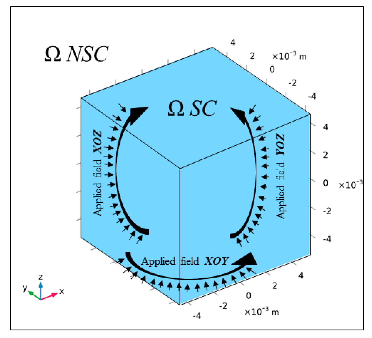
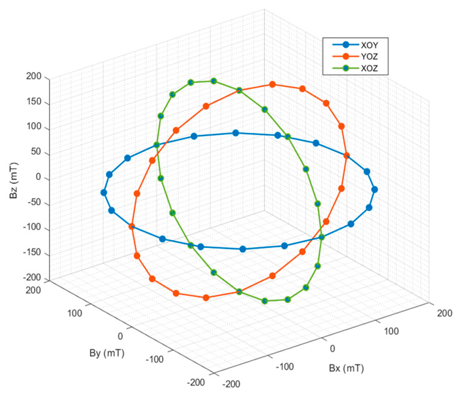
2.2. Rotating Magnetic Fields

The magnetic flux density vector B is typically restricted from flowing in the same direction as the magnetic field intensity H in 1D magnetic fields. In rotating electrical devices, however, the magnetic field rotates in a 2D plane, with B and H vectors that may or may not be in the same direction. The magnetic field is applied to the superconducting domain’s boundaries in this scenario. In the case of a 1D alternating field, a sine wave of the desired amplitude is introduced. The applied rotating magnetic field in the case of 2D rotating magnetization, on the other hand, is just a combination of sine waveforms at the boundaries of two separate axes, as per the testing criteria which may be expressed using the following equations:
                                    B 1 D a l t = B 0 sin ω t
B 2 D r o t = B 0 sin ω t                                                                                       B 0 sin ω t ± ( 1 exp t τ )  
where B 0 is the amplitude of the magnetic field, ω is the angular frequency, represents the phase shift angle, and τ is the time constant which is set as 0.05 s. A purely circular rotating field is created, which is usually obtained by shifting the phase angle of the second source by 90 degrees (i.e., π/2).
It should be noted that when a phase angle is moved along the axis, the magnetic field’s starting value is not equal to zero, causing an issue with the initial values in FEA and preventing the model from converging. As a result, in order to produce a transitory start, an exponential step function is applied in the second field source in Equation (10). In order to explore the electromagnetic properties of HTS bulks subjected to rotating magnetic fields, various 2D rotating flux density vectors in the XOY, XOZ, and YOZ planes are used in this study. At 200 mT, a purely circular rotating magnetic field surrounding the sample can be seen in Figure 2, which depicts the B Loci of various flux density patterns utilized in this investigation.

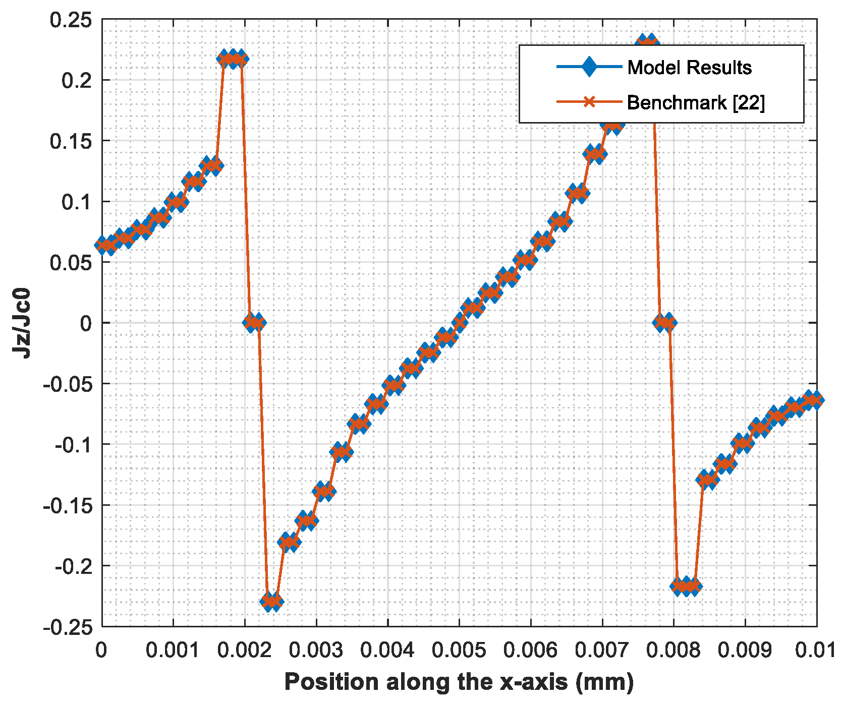
2.3. Model Validation

The same geometry was employed to perform this investigation in continuation with the benchmark study since the benchmark model of the cubic HTS sample is available for magnetization of the cubic sample on the z-axis. In order to validate the model, a sinusoidal magnetic field with an amplitude of 100 mT and frequency of 50 Hz is applied on the z-axis of the sample. The critical current density of the bulk superconductor is set as Jc0 = 108 A/m2. The current density ratio Jz/Jc0 along the x-axis at y = 2.07 mm and z = 1.1 mm is presented in Figure 3. As it can be observed, the simulation results are in good agreement with the benchmark solution [22]. Hence, the 3D modeling approach used in this article is thought to be accurate.

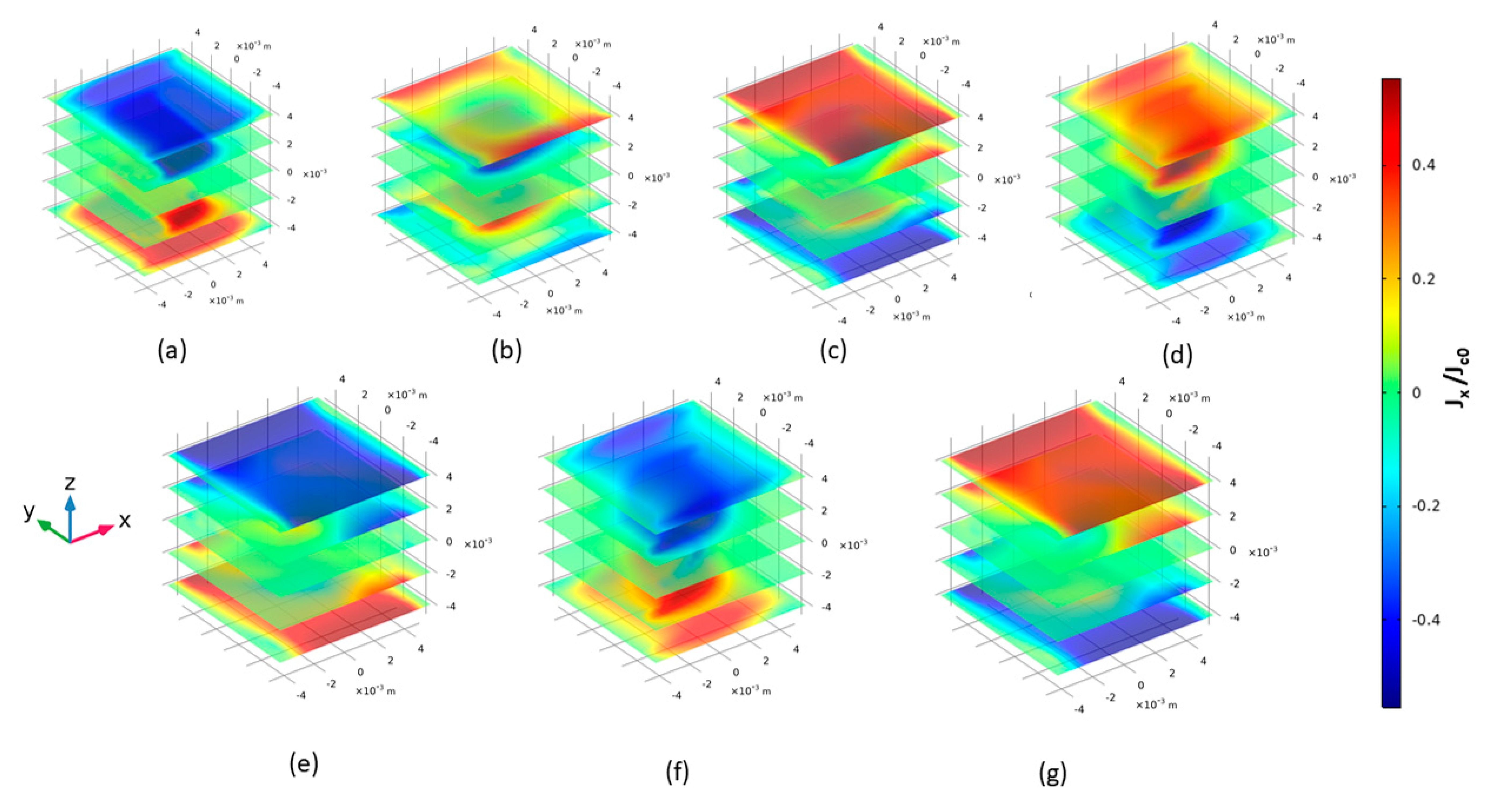
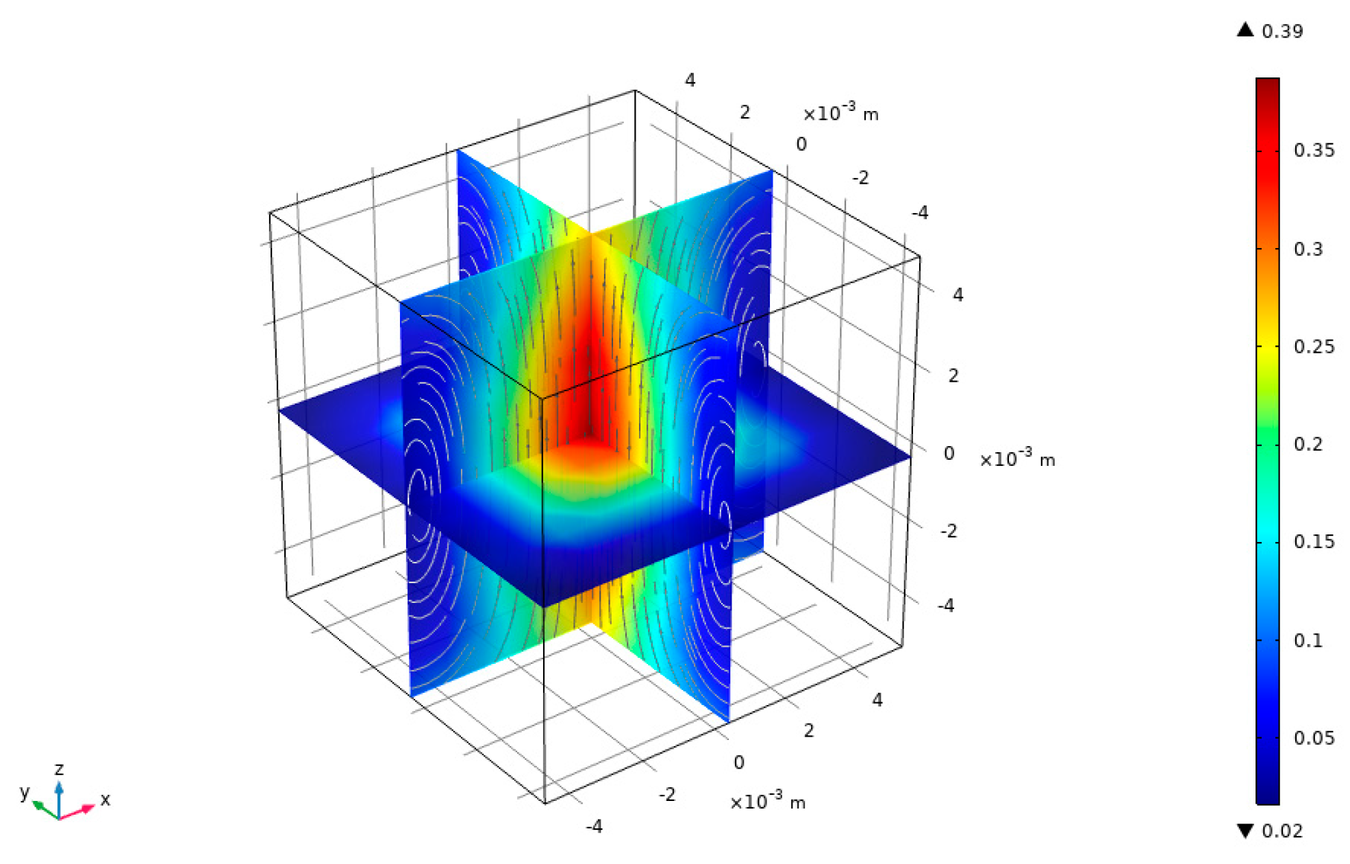
3. Magnetization of HTS

HTS trapped field magnets are alternative to permanent magnets but its investigation under rotating magnetic fields is not explicitly mentioned in the literature. Therefore, a thorough investigation of the movement of screening currents is indeed necessary. This study considers all finite-size effects with many layers of cells in the thickness. Since the 3D model technique allows current to flow in all three dimensions (x, y, and z), consequently, there is J for all three components (Jx; Jy; Jz).
In this section, the electromagnetic response of the HTS bulk subjected to rotating magnetic fields in XOY, XOZ, and YOZ with an amplitude of 200 mT is calculated using the model parameters mentioned in Section 2.

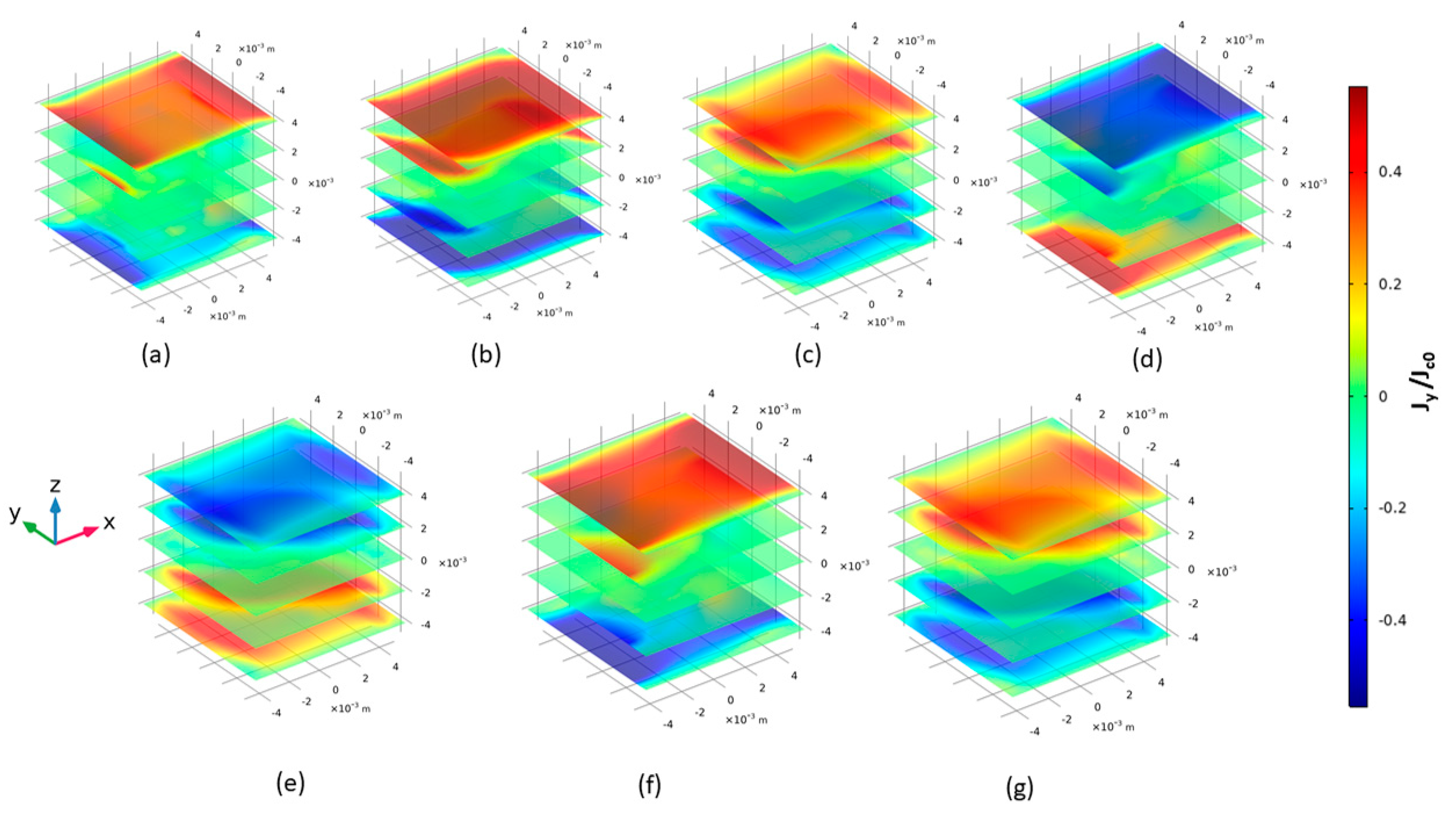
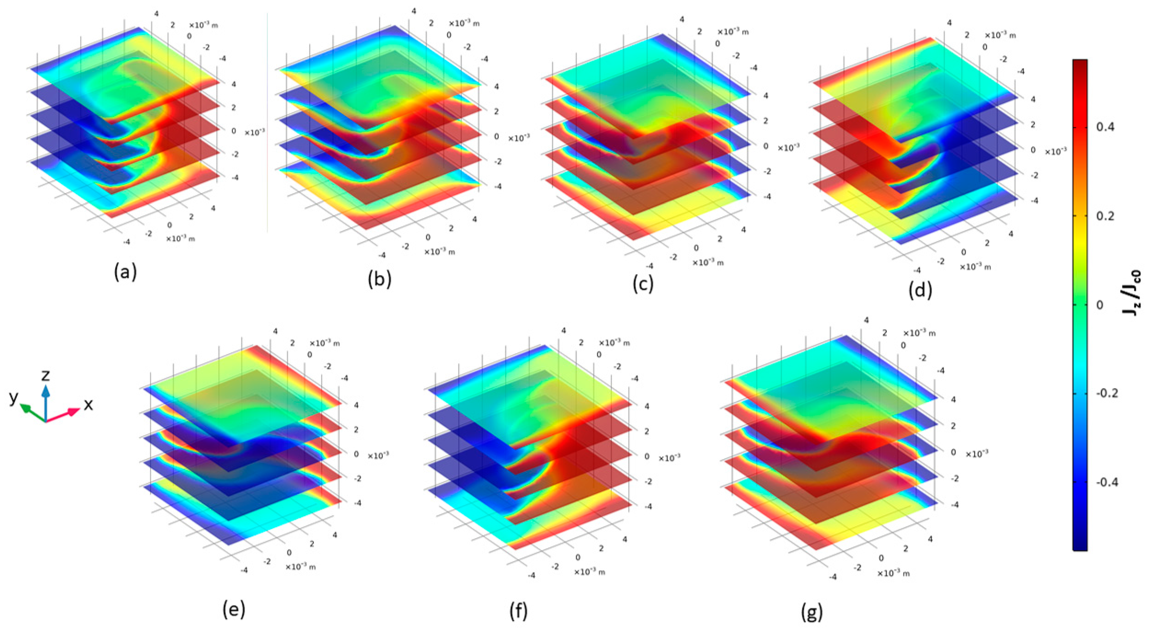
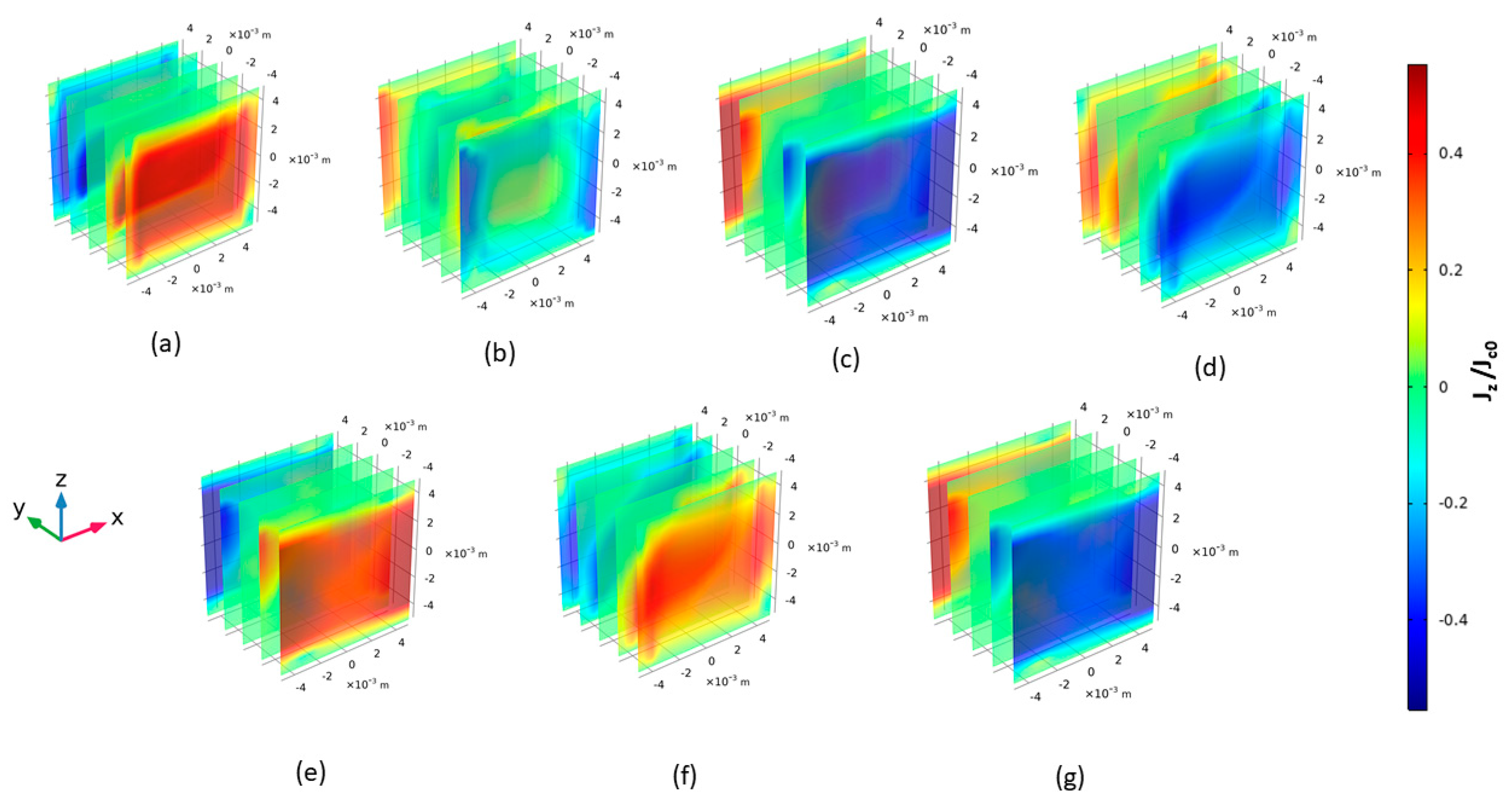
3.1. Magnetic Field Applied in XOY Plane

Figure 4, Figure 5 and Figure 6 show the 3D current density patterns when a rotating magnetic field of 20 mT in circular orientation is rotated in the XOY plane. The Jx component starts to penetrate from the z-axis of the sample and goes up to z = 20 mm at 15 ms with screening currents circulating in the radius of 20 mm. However, it settles at z = 40 mm with a value almost equal to 0.5 Jc0. Jy mostly remains on the surface around the z-axis, and a small current is penetrated up to 20 mm on the z-axis. Moreover, Jy is zero at z = 0 mm throughout the magnetizing process. The real rotating effect can be seen in the case of Jz where it starts from the surface of the y-axis and rotates all the way to z = 0 mm. The current density, in this case, is completely penetrated in the sample in a circular orientation, where the radius is decreased to zero along the magnetizing process.

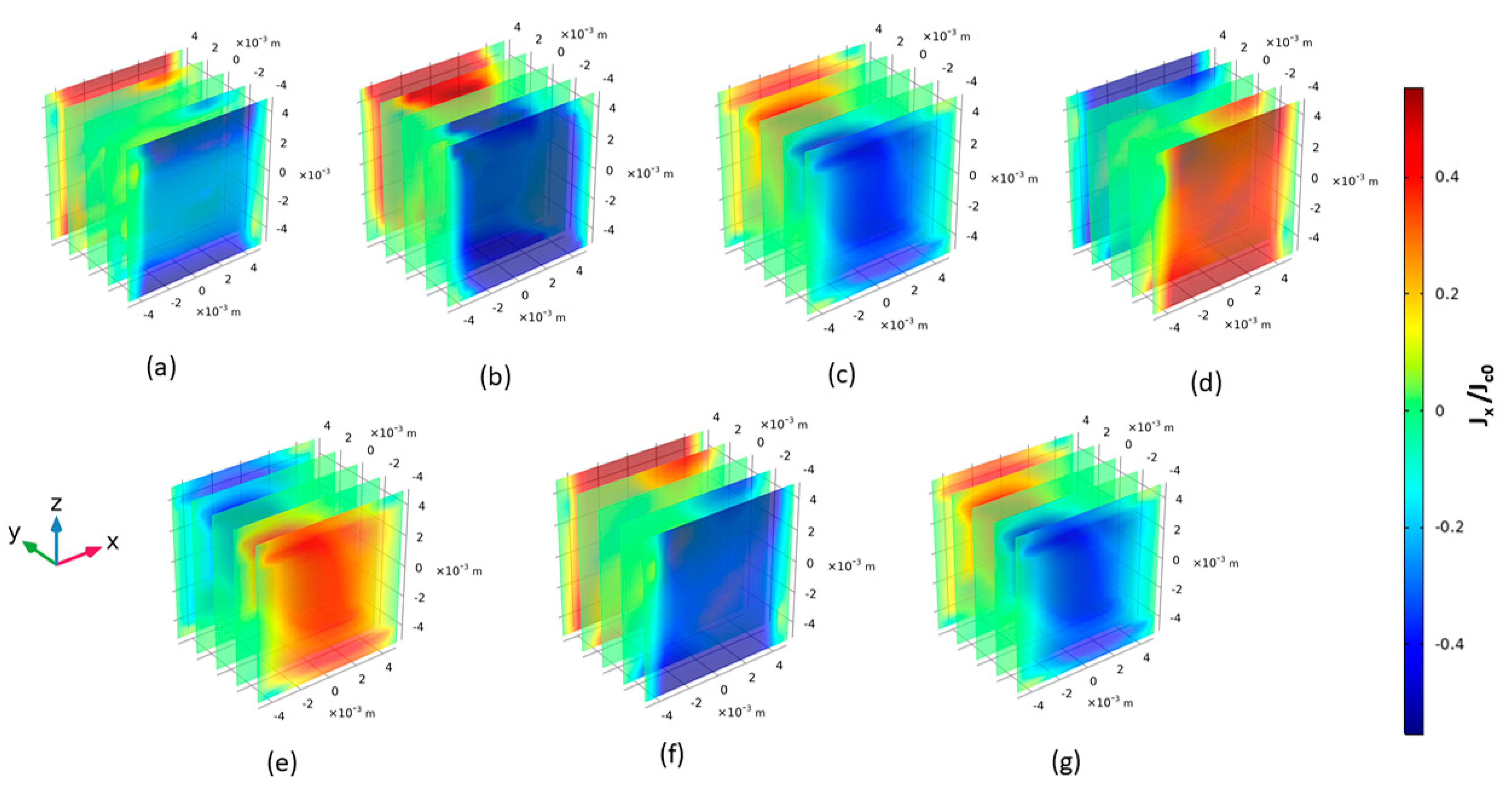
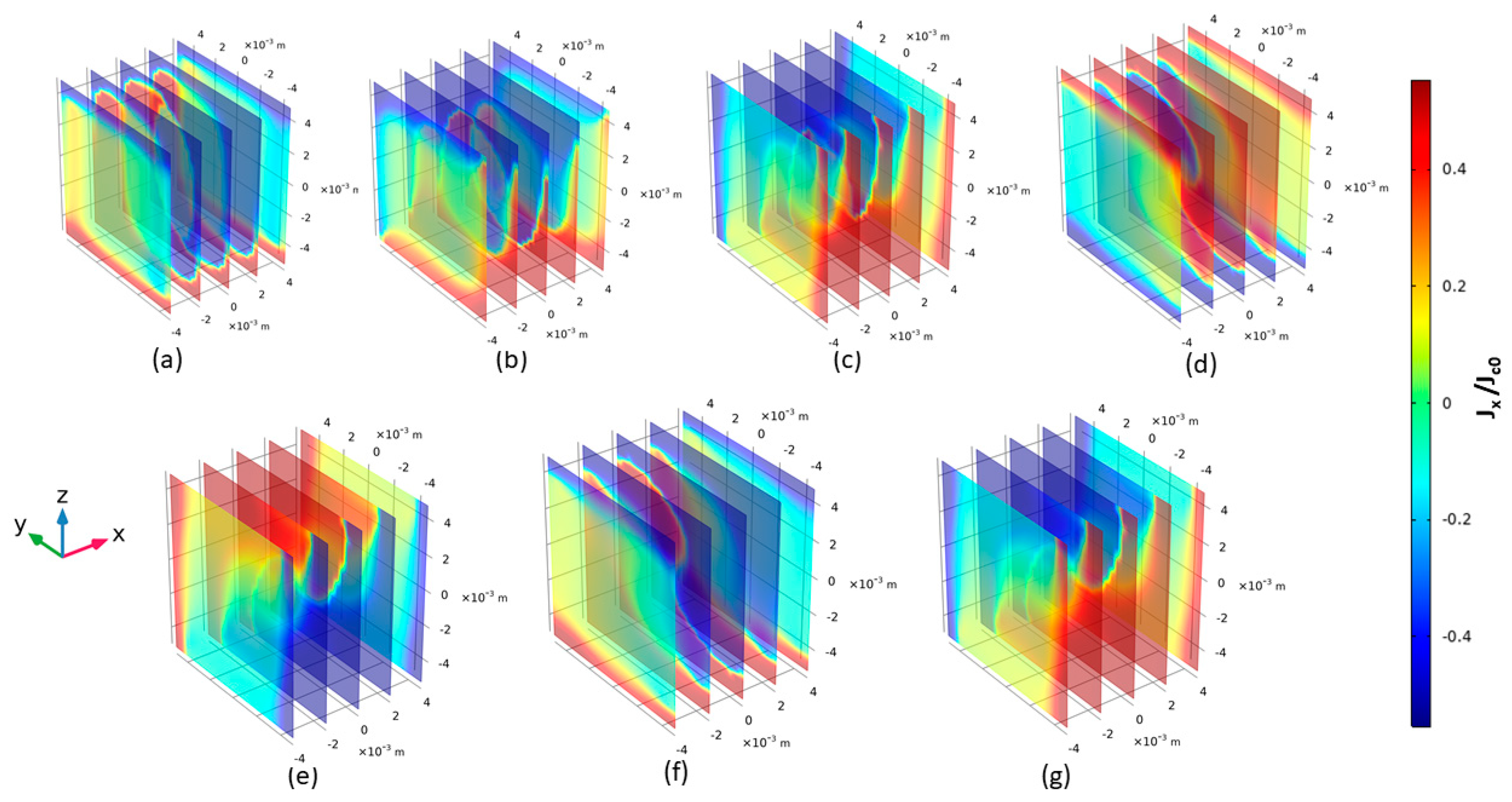
3.2. Magnetic Field Applied in XOZ Plane

Figure 7, Figure 8 and Figure 9 show the 3D current density patterns when a rotating magnetic field of 20mT in circular orientation is rotated in the XOZ plane. The Jx component shows a similar distribution pattern as Jx in XOY, but here, it starts to penetrate from the y-axis of the sample and goes up to y = 20 mm at 15 ms. However, it settles at y = 40 mm with a value almost equal to 0.5 Jc. Here, Jy mainly rotates around the X–Z plane, starting from the sides of the x-axis and settling on the sides of the z-axis. In this case, the screening currents are rotated in a circular orientation, but they do not completely penetrate inside the middle of the sample, unlike Jz in XOY. Jz stays mostly at the surface of the y-axis and penetrates only up to y = 20 mm.

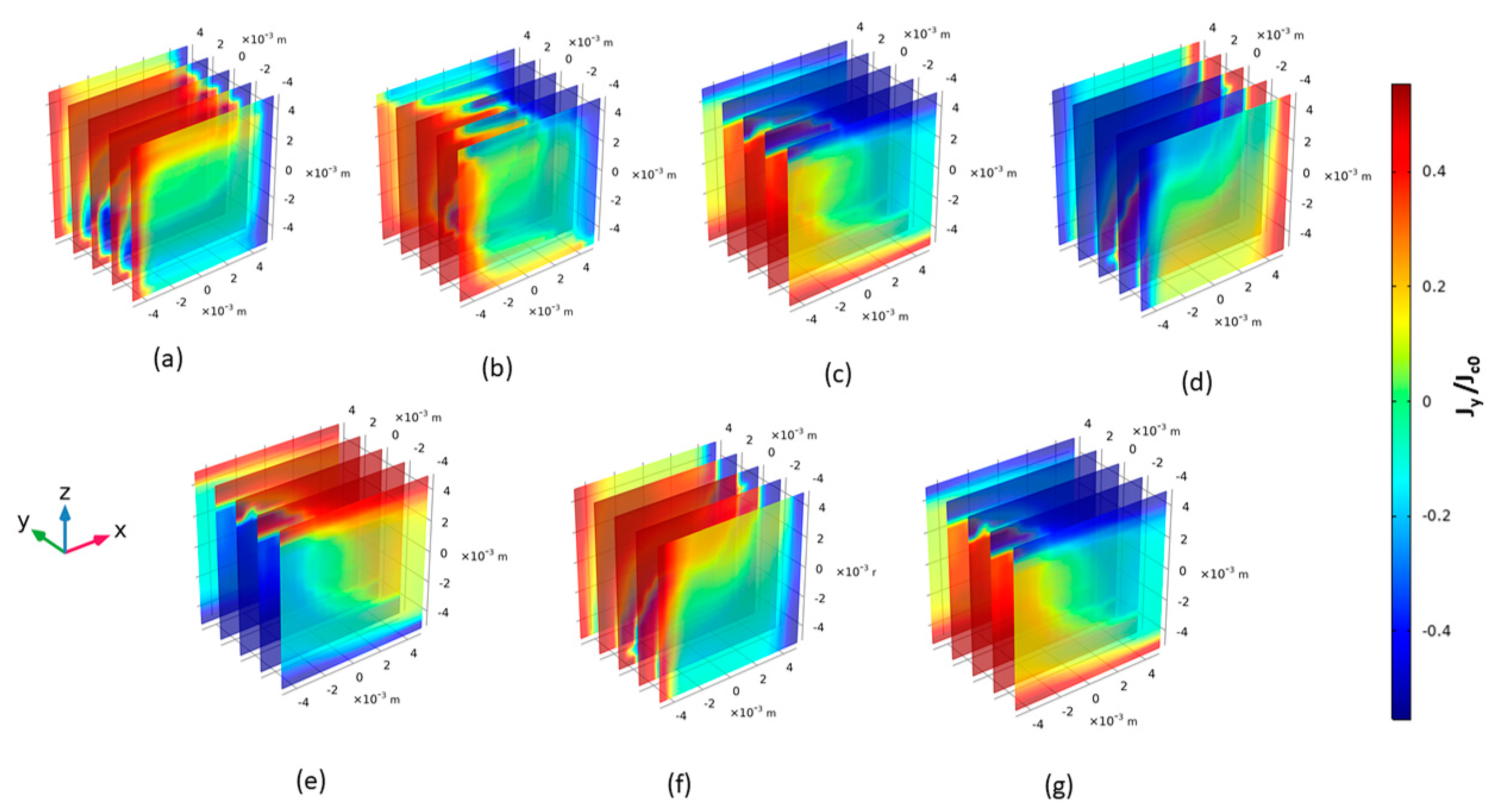
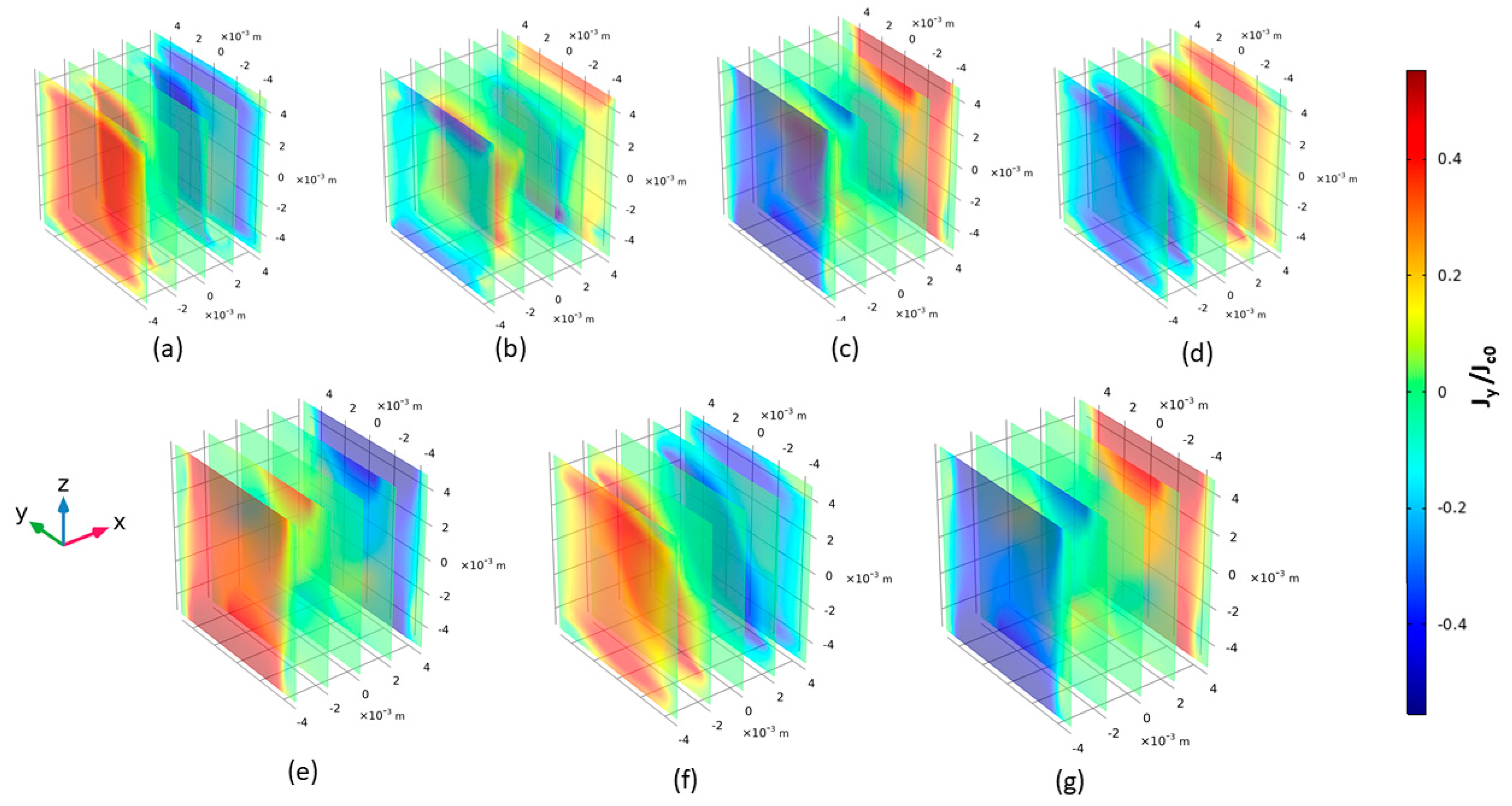
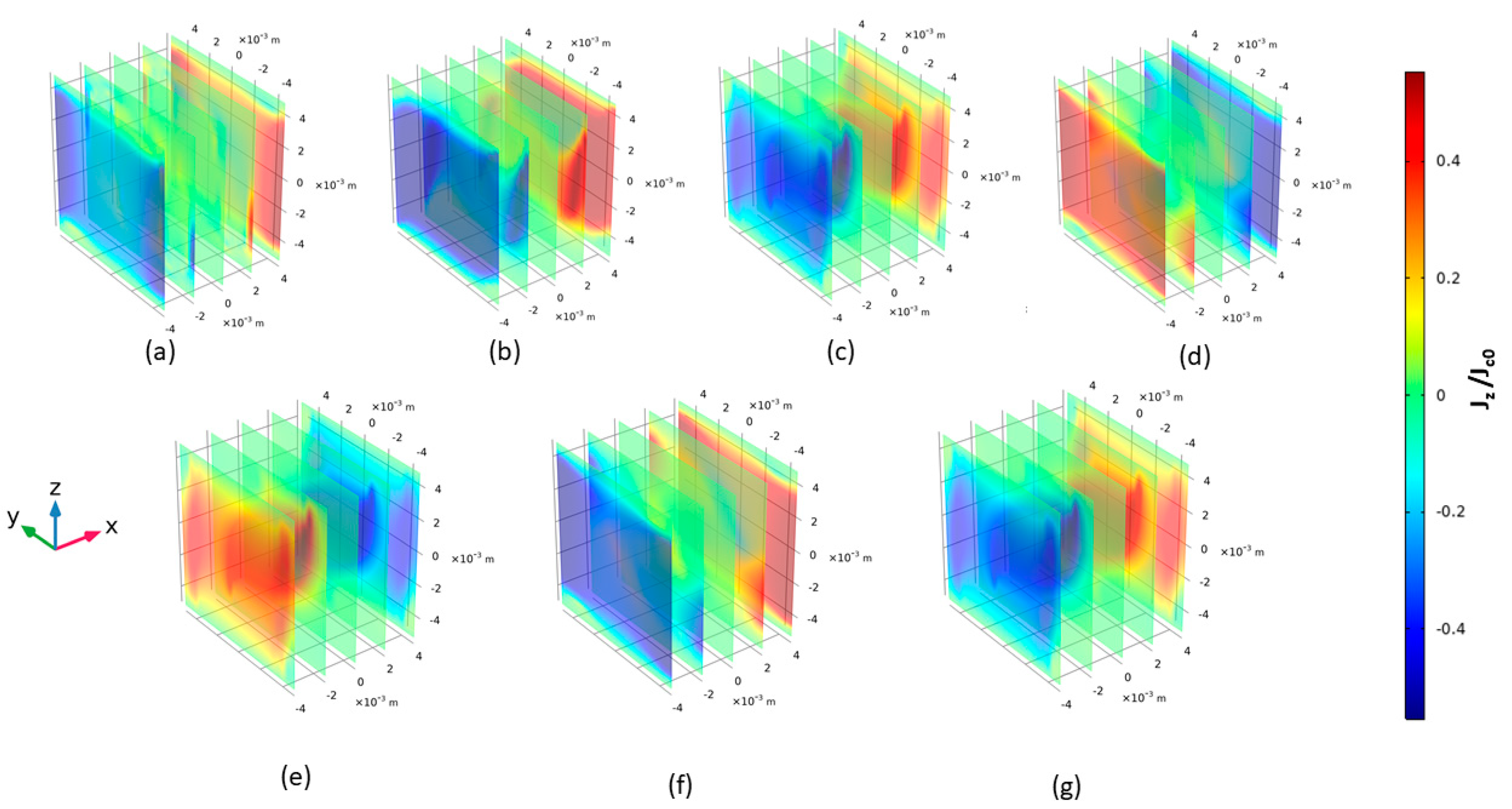
3.3. Magnetic Field Applied in YOZ Plane

Figure 10, Figure 11 and Figure 12 show the 3D current density patterns when a rotating magnetic field of 20 mT in circular orientation is rotated in the YOZ plane. Here, Jx mainly rotates around the Y–Z plane, starting from the sides of the z-axis and settling on the sides of the y-axis; the screening currents are rotated in a circular orientation, but they do not completely penetrate inside the middle of the sample, unlike Jz in XOY. The Jy component remains mostly on the sides of the x-axis. However, the Jz component starts to penetrate from the x-axis of the sample, goes up to z = 20 mm, and ultimately settles at z = 40 mm with a value almost equal to Jc. Jz mostly remains on the surface around the z-axis and shows exactly the same penetrating behavior as Jx in XOY.

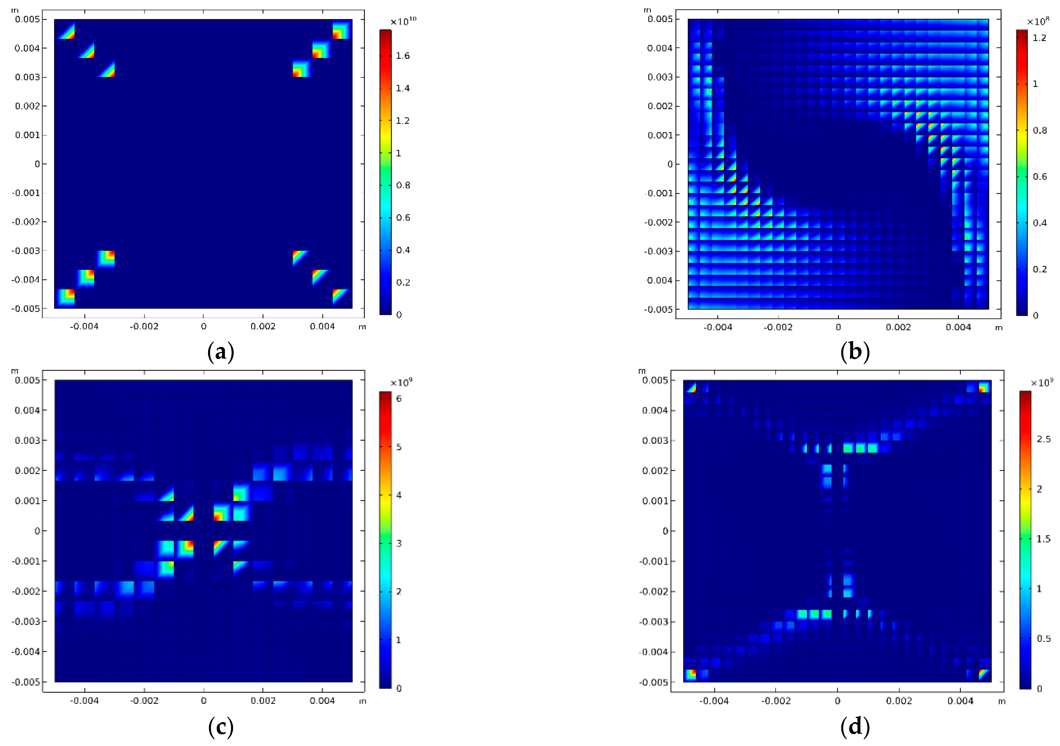
3.4. AC Loss Distribution

Figure 13 shows the AC loss distribution in the HTS bulk cubic sample when subjected to a rotating magnetic field of 20 mT. In order to compare the results, the AC loss of 1D magnetization in the z-axis is also mentioned in Figure 13a, followed by XOY, XOZ, and YOZ in (b), (c), and (d), respectively, at z = 5 mm. The AC loss in 1D magnetization appears mainly in the sample’s diagonals up to 3 mm from each corner. The AC loss is circulated along the sides of the sample when the magnetic field is applied in XOY. However, the AC loss seems to be distributed in the middle of the sample as well as in the case of XOZ and YOZ. From the distribution patterns it can be analyzed that the AC loss is increased significantly when the HTS bulk sample is subjected to rotating magnetic fields in comparison with the one-dimensional alternating magnetic field. It should be noted that the loss distribution is captured at the same geometrical orientation to understand the pattern of distribution upon magnetizing in different axes. A detailed analysis of AC loss under various amplitudes and orientations of rotating magnetic fields is presented in [23].

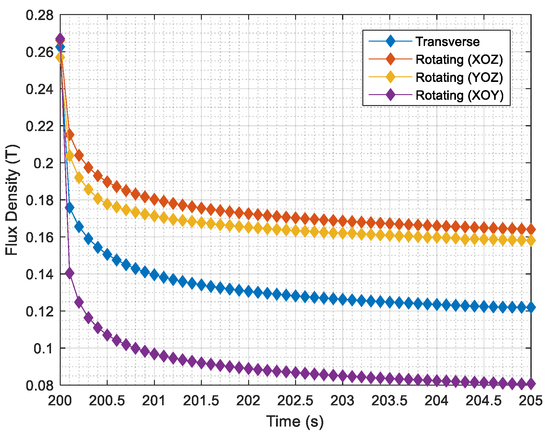
4. Demagnetization of HTS Trapped Field Magnets

HTS trapped field magnets have shown promising applications to be used as a substitute for permanent magnets in various large-scale applications. However, the application of external magnetic fields on HTS permanent magnets significantly decreases the trapped field. There are a lot of demagnetization studies published on demagnetization through transverse or cross-field demagnetization, but demagnetization through rotating magnetic fields is not reported anywhere. In this section, we have investigated the demagnetization behavior of HTS permanent magnets under applied rotating magnetic fields in various orientations. The 3D model can produce accurate results by considering a finite sample size including end effects. The demagnetization investigation has two parts. The first part is very important, where the sample will be magnetized to trap the magnetic field in order to become a trapped field magnet. In the second part, the trapped field magnet is demagnetized by rotating magnetic fields in different orientations.
For the first part of the study, the cubic sample is magnetized by field cooling method, considering the sample is already cooled to its critical temperature [24]. The initial applied magnetic field is 1 T with a ramp-down rate of 10 mT/s. Afterward, a relaxation time is initiated to stabilize the trapped magnetic field. Figure 14 shows the magnetic field trapped in the HTS bulk sample after the relaxation time. The trapped magnetic field of the sample is 0.27 T, which is computed at the center of the top surface, similar to the Hall probe measurement. Parameters specific for demagnetization are mentioned in Table 2. The rest of the modeling parameters remain the same as per Table 1.
Once the magnetic field is stabilized in the sample after relaxation time, the sample is exposed to various patterns of external magnetic fields of 0.1 T to see the demagnetizing effect. In order to compare the demagnetization through 1D magnetic fields, a transverse magnetic field is also applied in the y-direction. The effect of demagnetization is presented in Figure 15.
When the magnetic field is applied in the transverse direction, the sample is demagnetized to 0.12 T. The rotating magnetic fields in XOZ and YOZ orientations result in 0.17 T and 0.16 T, which is slightly higher than the transverse direction. This may be due to the fact that the sample is already magnetized in z-orientation, and the applied magnetic field could be parallel to the direction of the trapped field. However, when the field is rotated around the XOY plane, there is a significant decrease up to 0.8 T in the trapped field, mainly due to the application of a magnetic field perpendicular to the trapped magnetic field.

5. Conclusions

In this study, we have analyzed and characterized the electromagnetic properties of HTS bulks using 3D numerical modeling techniques under the exposure of rotating magnetic fields in XOY, XOZ, and YOZ planes. To explain all finite-size effects, complete 3D computational methods for nonlinear superconducting materials are required. Since power devices are finite in size, the finite-size effects aid in understanding and optimizing superconductors in power applications. The interpretation of characterization and measurement is also influenced by finite-size effects. The 3D numerical model provides realistic predictions considering all finite-size effects with a huge number of degrees of freedom. The typical current density distribution J and AC loss distribution profiles are presented for all three components (Jx; Jy; Jz) under the influence of a rotating magnetic field in different orientations. The demagnetization subjected to similar rotating fields is also investigated to see how the HTS trapped field magnets are demonized, which is also a very important characteristic for their applications as alternate candidates to permanent magnets. The performance of the model has been verified with the available benchmark of the HTS cubic bulk sample. The electromagnetic data presented in this study will provide a comprehensive understating of the material properties of HTS when subjected to rotating magnetic fields.
Although numerical models are powerful tools to predict the performance of HTS materials, experimental techniques are also really important for the investigation of HTS electromagnetic properties. Nevertheless, there is lack of robust experimental methods for predicting material properties under rotating magnetic fields, especially AC loss. In future work, such an experimental technique shall be proposed to predict the rotating AC loss mechanism in order to fully understand the material properties.

Author Contributions

Conceptualization, W.A.S., Y.G. and J.Z.; Methodology, W.A.S., B.S.; Software, W.A.S., B.S.; Supervision, Y.G. and H.L.; Visualization, W.A.S., Y.G., J.Z.; Writing—original draft, W.A.S. and Y.G.; Writing—review & editing, H.L., J.Z., J.J. and B.S. All authors have read and agreed to the published version of the manuscript.

Funding

This research was funded by Australian Research Council Discovery Project DP180100470.

Institutional Review Board Statement

Not applicable.

Informed Consent Statement

Not applicable.

Data Availability Statement

Not applicable.

Conflicts of Interest

The authors declare no conflict of interest.

References

  1. Soomro, W.A.; Guo, Y.; Lu, H.Y.; Jin, J.X. Advancements and Impediments in Applications of High-Temperature Superconducting Material. In Proceedings of the 2020 IEEE International Conference on Applied Superconductivity and Electromagnetic Devices (ASEMD), Tianjin, China, 16–18 October 2020; pp. 1–4. [Google Scholar] [CrossRef]
  2. Zhang, M. A new world record for a superconducting trapped field magnet. Supercond. Sci. Technol. 2019, 32, 070502. [Google Scholar] [CrossRef]
  3. Zhou, D.; Izumi, M.; Miki, M.; Felder, B.; Ida, T.; Kitano, M. An overview of rotating machine systems with high-temperature bulk superconductors. Supercond. Sci. Technol. 2012, 25, 103001. [Google Scholar] [CrossRef]
  4. Bause, R.; Ainslie, M.D.; Corduan, M.; Boll, M.; Filipenko, M.; Noe, M. Electromagnetic design of a superconducting electric machine with bulk HTS material. arXiv 2019, arXiv:1903.08906. [Google Scholar]
  5. Moon, H.; Kim, Y.-C.; Park, H.-J.; Park, M.; Yu, I.-K. Development of a MW-Class 2G HTS Ship Propulsion Motor. IEEE Trans. Appl. Supercond. 2016, 26, 5203805. [Google Scholar] [CrossRef]
  6. Chen, W.; Xu, Y.; Wang, Z.; Ren, L.; Shi, J.; Tang, Y. Levitation Force Computation of HTS/PM System Based on $H$ -Formulation. IEEE Trans. Magn. 2018, 54, 7402805. [Google Scholar] [CrossRef]
  7. Braginski, A.I. Superconductor Electronics: Status and Outlook. J. Supercond. Nov. Magn. 2018, 32, 23–44. [Google Scholar] [CrossRef] [Green Version]
  8. Zan, G.; Wu, T.; Zhu, F.; He, P.; Cheng, Y.; Chai, S.; Wang, Y.; Huang, X.; Zhang, W.; Wan, Y.; et al. A biomimetic conductive super-foldable material. Matter 2021, 4, 3232–3247. [Google Scholar] [CrossRef]
  9. Zan, G.; Wu, T.; Zhang, Z.; Li, J.; Zhou, J.; Zhu, F.; Chen, H.; Wen, M.; Yang, X.; Peng, X.; et al. Bioinspired Nanocomposites with Self-Adaptive Stress Dispersion for Super-Foldable Electrodes. Adv. Sci. 2021, 9, 2103714. [Google Scholar] [CrossRef]
  10. Smith, J.P.; Mazin, B.A.; Walter, A.B.; Daal, M.; Bailey, J.I.; Bockstiegel, C.; Zobrist, N.; Swimmer, N.; Steiger, S.; Fruitwala, N. Flexible Coaxial Ribbon Cable for High-Density Superconducting Microwave Device Arrays. IEEE Trans. Appl. Supercond. 2020, 31, 2500105. [Google Scholar] [CrossRef]
  11. Huang, J.; Wang, H.; Wang, H.; Zhang, B.; Qian, X.; Wang, H. Superconducting Iron Chalcogenide Thin Films Integrated on Flexible Mica Substrates. IEEE Trans. Appl. Supercond. 2019, 29, 7500604. [Google Scholar] [CrossRef]
  12. Gimaev, R.; Spichkin, Y.; Kovalev, B.; Kamilov, K.; Zverev, V.; Tishin, A. Review on magnetic refrigeration devices based on HTSC materials. Int. J. Refrig. 2019, 100, 1–12. [Google Scholar] [CrossRef]
  13. Vanderbemden, P.; Hong, Z.; Coombs, T.A.; Ausloos, M.; Babu, N.H.; Cardwell, D.A.; Campbell, A.M. Remagnetization of bulk high-temperature superconductors subjected to crossed and rotating magnetic fields. Supercond. Sci. Technol. 2007, 20, S174–S183. [Google Scholar] [CrossRef]
  14. Qiu, M.; Lin, L.; Zhang, G.; Wang, Y.; Xiao, L. Flux dynamic behavior inside HTS bulks under rotating magnetic field. IEEE Trans. Appl. Supercond. 2002, 12, 1163–1166. [Google Scholar] [CrossRef]
  15. Qiu, M.; Huo, H.; Xu, Z.; Xia, D.; Lin, L. Electromagnetic Phenomena in HTS Bulk Subjected to a Rotating Field. IEEE Trans. Appl. Supercond. 2004, 14, 1898–1901. [Google Scholar] [CrossRef]
  16. Lousberg, G.P.; Ausloos, M.; Geuzaine, C.; Dular, P.; Vanderbemden, P.; Vanderheyden, B. Numerical simulation of the magnetization of high-temperature superconductors: A 3D finite element method using a single time-step iteration. Supercond. Sci. Technol. 2009, 22, 055005. [Google Scholar] [CrossRef]
  17. Amemiya, N.; Murasawa, S.-I.; Banno, N.; Miyamoto, K. Numerical modelings of superconducting wires for AC loss calculations. Phys. C Supercond. 1998, 310, 16–29. [Google Scholar] [CrossRef]
  18. Escamez, G.; Sirois, F.; Lahtinen, V.; Stenvall, A.; Badel, A.; Tixador, P.; Ramdane, B.; Meunier, G.; Perrin-Bit, R.; Bruzek, C.-E. 3-D Numerical Modeling of AC Losses in Multifilamentary MgB2Wires. IEEE Trans. Appl. Supercond. 2016, 26, 4701907. [Google Scholar] [CrossRef]
  19. Shen, B.; Grilli, F.; Coombs, T. Overview of H-Formulation: A Versatile Tool for Modeling Electromagnetics in High-Temperature Superconductor Applications. IEEE Access 2020, 8, 100403–100414. [Google Scholar] [CrossRef]
  20. Shen, B.; Grilli, F.; Coombs, T. Review of the AC loss computation for HTS using H formulation. Supercond. Sci. Technol. 2020, 33, 033002. [Google Scholar] [CrossRef] [Green Version]
  21. Bean, C.P. Magnetization of Hard Superconductors. Phys. Rev. Lett. 1962, 8, 250–253. [Google Scholar] [CrossRef]
  22. HTS MODELLING WORKGROUP. Available online: http://www.htsmodelling.com/ (accessed on 10 January 2022).
  23. Soomro, W.A.; Guo, Y.; Lu, H.Y.; Zhu, J.G.; Jin, J.X.; Shen, B. Numerical Investigation of AC Loss in HTS Bulks Subjected to Rotating Magnetic Fields. In Proceedings of the 2021 31st Australasian Universities Power Engineering Conference (AUPEC), Perth, Australia, 26–30 September 2021; pp. 1–5. [Google Scholar] [CrossRef]
  24. Zou, S.; Zermeno, V.M.R.; Grilli, F. Simulation of Stacks of High-Temperature Superconducting Coated Conductors Magnetized by Pulsed Field Magnetization Using Controlled Magnetic Density Distribution Coils. IEEE Trans. Appl. Supercond. 2016, 26, 8200705. [Google Scholar] [CrossRef] [Green Version]
Figure 1. Geometry of the HTS bulk sample. Ω SC is the superconducting region, and Ω NSC is the non-superconducting air domain. The magnetic fields are applied in XOY, XOZ, and YOZ planes.
Energies 15 03186 g001
Figure 2. Loci of flux density for flux density vectors XOY, XOZ, and YOZ.
Energies 15 03186 g002
Figure 3. Jz/Jc0 along the x-axis at y = 2.07 mm and z = 1.1 mm for the benchmark cubic bulk superconductor model and the model built in this study. The benchmark solution is obtained using MEMEP and the relevant data are extracted from benchmark [22].
Energies 15 03186 g003
Figure 4. Component of current density Jx subjected to 200 mT in XOY plane at (a) 1 ms, (b) 3 ms, (c) 5 ms, (d) 10 ms, (e) 15 ms, (f) 20 ms, and (g) 25 ms.
Energies 15 03186 g004
Figure 5. Component of current density Jy subjected to 200 mT in XOY plane at (a) 1 ms, (b) 3 ms, (c) 5 ms, (d) 10 ms, (e) 15 ms, (f) 20 ms, and (g) 25 ms.
Energies 15 03186 g005
Figure 6. Component of current density Jz subjected to 200 mT in XOY plane at (a) 1 ms, (b) 3 ms, (c) 5 ms, (d) 10 ms, (e) 15 ms, (f) 20 ms, and (g) 25 ms.
Energies 15 03186 g006
Figure 7. Component of current density Jx subjected to 200 mT in XOZ plane at at (a) 1 ms, (b) 3 ms, (c) 5 ms, (d) 10 ms, (e) 15 ms, (f) 20 ms, and (g) 25 ms.
Energies 15 03186 g007
Figure 8. Component of current density Jy subjected to 200 mT in XOZ plane at (a) 1 ms, (b) 3 ms, (c) 5 ms, (d) 10 ms, (e) 15 ms, (f) 20 ms, and (g) 25 ms.
Energies 15 03186 g008
Figure 9. Component of current density Jz subjected to 200 mT in XOZ plane at at (a) 1 ms, (b) 3 ms, (c) 5 ms, (d) 10 ms, (e) 15 ms, (f) 20 ms, and (g) 25 ms.
Energies 15 03186 g009
Figure 10. Component of current density Jx subjected to 200 mT in YOZ plane at (a) 1 ms, (b) 3 ms, (c) 5 ms, (d) 10 ms, (e) 15 ms, (f) 20 ms, and (g) 25 ms.
Energies 15 03186 g010
Figure 11. Component of current density Jy subjected to 200 mT in YOZ plane at (a) 1 ms, (b) 3 ms, (c) 5 ms, (d) 10 ms, (e) 15 ms, (f) 20 ms, and (g) 25 ms.
Energies 15 03186 g011
Figure 12. Component of current density Jz subjected to 200 mT in YOZ plane at (a) 1 ms, (b) 3 ms, (c) 5 ms, (d) 10 ms, (e) 15 ms, (f) 20 ms, and (g) 25 ms.
Energies 15 03186 g012
Figure 13. AC loss distribution in (a) 1-D z-axis, (b) XOY plane, (c) XOZ plane, and (d) YOZ plane.
Energies 15 03186 g013
Figure 14. The trapped field in HTS permanent magnet.
Energies 15 03186 g014
Figure 15. Demagnetization in HTS trapped field subjected to rotating magnetic field.
Energies 15 03186 g015
Table 1. Model Parameters.
ParameterSymbolValue
Permeability of free spaceμ04π × 10−7 H.m−4
Power Factorn25
Critical Current DensityJc0108 A.m−2
Characteristic Electric FieldE010−4 V m−1
Kim’s Model Arbitary ParameterB00.0041 T
Kim’s Model Arbitary Parameterm0.5
Table 2. Model Parameters.
ParameterValue
Magnetizing Field1 T
Ramp down rate of magnetizing0.01 T/s
Magnetizing time100 s
Time to allow for flux creep (Relaxation time)100 s
Demagnetizing time5 s
Publisher’s Note: MDPI stays neutral with regard to jurisdictional claims in published maps and institutional affiliations.

