Post-Optimum Sensitivity Analysis with Automatically Tuned Numerical Gradients Applied to Swept Wind Turbine Blades

Abstract

Post-Optimum Sensitivity Analysis (POSA) extends numerical design optimization to provide additional information on how the design and performance would change if various parameters and constraints were varied. POSA is challenging since it typically requires accurate gradients and gradient-based optimization problems that provide Lagrange multipliers. To overcome this problem, this paper introduces a technique to automatically tune gradients with statistical methods and algorithms to calculate the Lagrange multipliers after an optimization. This allows these methods to be applied to problems with noisy gradients or problems solved with gradient-free optimization algorithms. These methods have been applied to swept wind turbine blades. Swept blades can reduce wind turbine loads by twisting out of the wind when the wind speed increases. The methods have shown that introducing design freedom in the sweep, blade root flap-wise bending moments and blade tip deflection has a weaker influence on the design. Instead, blade root torsion moment and material failure become the driving constraints.

1. Introduction

Numerical design optimization has been successfully applied to wind turbine blade design within the research community several times [1,2,3,4]. In all of these cases, the focus of the analysis was on the optimal design itself and not on the optimization problem. Any given optimization problem is based on a set of chosen constraint limits and assumed parameter values that, in turn, reflect previous design decisions. For example, the choice of material defines the strength limits, the choice of wind conditions affects both the production and the loads. Thus, numerical design optimization must still be embedded within a human-driven design process, where questions on how the different constraints and parameters affect the design can be just as important as the final design itself. Knowledge of the most important constraints and parameters can help guide design engineers and researchers towards improvements that will have the most impact on the design in the larger human-driven design process. To help guide this process, POSA can inform design engineers on how changes to the optimization problem may affect the final outcome.

POSA has already been established within the optimization community [5]. Furthermore, Sobieszczanski-Sobieski et al. [6] applied POSA to aerospace optimization problems in 1982. POSA is also commonly applied for structural optimization problems in civil engineering to obtain more effective solutions (e.g., Nishat et al. [7]). Yet POSA is rarely used within the wind energy community. So this paper aims to introduce POSA with an optimum wind turbine blade design. In the most basic application, post-sensitivity analysis shows how the objective would change with changes in the constraint limits, which can be used to judge what constraints are most important. Typically, constraint limits are not the only set of chosen constants, various parameters are also used (e.g., different wind classes, assumptions on tilt and coning). Furthermore, understanding how design solution itself changes with respect to parameters and constraint limits may be more important than changes in the objective value. POSA can also be extended to determine how both the objective and the design solution would change with respect to both constraint limits and assumed parameter values.

The basic application of POSA is based on the Lagrange multipliers in the Karush-Kuhn-Tucker (KKT) conditions, which in some cases is part of the output in the optimization. Yet, gradient-free optimization and surrogate-based optimization methods [8] do not provide this information readily. The review article by Sawant et al. [9] cites a large body of work that use gradient-free methods that could benefit from additional POSA post-processing methods. Furthermore, extending POSA to include sensitivity of the design solution and sensitivity with respect to parameters requires additional analysis beyond the Lagrange multipliers given by the optimization itself [10]. This paper introduces an extended POSA method that can be applied after the optimization.

An additional challenge in applying POSA is that it requires accurate gradients, fully converged optimal solutions, and in some cases, second-order gradient information [5]. However, many of the analysis tools within wind energy do not provide design sensitivity analysis. Instead, many optimization frameworks rely on inaccurate numerical gradients like the finite difference. The consequences of inaccurate gradients within wind energy have been discussed by many authors [11,12,13], showing that these errors can lead to poor convergence. In finite difference, one must choose a step parameter; if this parameter is too small, a round-off error is introduced, and if too large, a truncation error is introduced. For problems with very large Jacobians, it is impractical to tune the step size manually. The problem of tuning finite difference step-size has recently received attention from the machine learning community, where methods for stochastic gradient descent methods have been developed by Castera et al. [14] along with adaptive methods by Mahmood et al. [15]. Instead, this paper introduces a more generic approach based on statistical methods for automatically tuning the finite difference gradients.

In wind turbine rotor design, the objective maximizes energy production without exceeding load limits. Typically if one can reduce the loads, production can be improved by extending the rotor. Accordingly, much research has been applied to two different passive load alleviation techniques. The first leverages the anisotropy of fiber-reinforced materials to achieve bend-twist coupling, with many examples within literature [16,17,18,19,20,21,22]. The second leverages swept blade geometry to achieve bend-twist coupling, with additional examples in the literature [23,24,25,26,27]. A few studies have tried to compare these methods [20,21]. Recently the authors of this paper have applied numerical design optimization on a 100 kW rotor to show that there is greater potential in swept blades over elastically coupled blades [28].

Most of the research into load alleviation has not applied POSA to understand how the larger design problem has been affected by the new design freedom. Engineering design is a matter of trade-offs, which cannot always be apparent with a single optimal design. With POSA, one can see how the different trade-offs are changed by introducing new design freedom to the problem. This paper will demonstrate POSA on both the straight and swept blade optimization solutions of [28], to understand how the design drivers change when sweeping is introduced.

This paper is organized as follows: First, much of the analysis is based on the optimization given by McWilliam et al. [28], so the paper starts with a very short summary of this work in Section 2 to give context to the following examples. Then, the paper introduces statistical techniques that were used to automatically tune the finite difference gradients in Section 3. These gradients were only used in the subsequent POSA and not in the optimization. The POSA methods are given in Section 4. Finally, the results of these methods on straight and swept designs are compared in Section 5.

2. Rotor Blade Optimization

This work is based on the optimization results taken from McWilliam et al. [28]. This section is meant to give only the details that are relevant for the analysis in this work. In the original optimization study, three different 100 kW blade optimization problems were solved, a conventional straight blade, a material coupled blade, and a swept blade. Only the preliminary straight and swept blade results were analyzed in this work.

In both optimizations, the objective was to maximize the Annual Energy Production (AEP), without increasing the loads. The design variables were composed of a mix of aerodynamic planform variables, internal structural variables, and control variables. The design variables of interest in this work are the blade length, chord, twist, relative thickness, sweep, pre-bend, pitch axis, spar-cap laminate thickness, spar-cap width, trailing edge panel uniaxial laminate thickness, leading-edge panel uniaxial laminate thickness. The constraints of interest in this work were the blade root flap-wise bending moment, thrust, blade tip deflection, mass, blade failure, torsion, and a geometric constraint on the maximum allowed sweep. The optimization also had a large number of simple geometric constraints to avoid degenerate configurations (e.g., maximum chord, avoiding negative thicknesses). The optimization was based on a large collection of input data that was held constant in the optimization. The analysis presented in this work looked at the impact of varying airfoil drag, the maximum lift of the airfoils, material stiffness characteristics, gust strength used in the loads’ analysis, and material failure properties.

More details about the optimal designs can be found in [28].

3. Finite Difference Gradient Tuning

Gradients are needed in both post-optimum sensitivity analysis and gradient-based optimization, yet typically engineering analysis codes do not provide these gradients. Instead, these gradients are estimated with finite difference, for example the first order backwards differencing, second-order central differencing and first-order forward differencing in Equations (1)–(3), respectively. These schemes are based on a step length parameter h, while at the same time subject to round-off error for small values of h and truncation error for large values of h. Thus, estimating an accurate gradient requires selecting the correct step length where the combined effect of these errors is minimized.

$$\frac{df}{dx}\approx \frac{f\left(x\right)-f(x-h)}{h}$$

(1)

$$\frac{df}{dx}\approx \frac{f(x+h)-f(x-h)}{2h}$$

(2)

$$\frac{df}{dx}\approx \frac{f(x+h)-f\left(x\right)}{h}$$

(3)

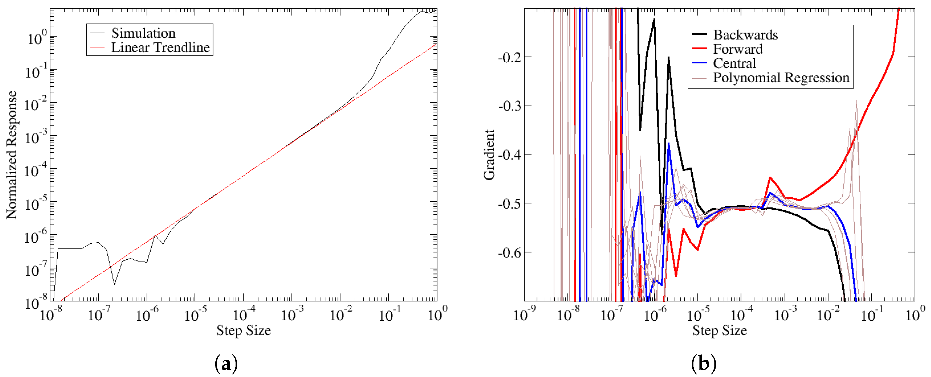
Figure 1a shows the blade failure constraint values with respect to perturbations to the spar-cap uniaxial laminate thickness. The response is normalized according to $\overline{r}=|r-r_0|$ where r is the perturbed response value, $r_0$ is the response value of the unperturbed design. The corresponding finite-difference gradients are shown in Figure 1b, along with additional estimates from polynomial regression (see below for details on the polynomial regression). From these figures, it is obvious that the best estimation occurs when the different numerical gradient schemes give good agreement with each other. Without analytic gradients, the exact error in the numerical gradients cannot be determined. Instead, we assume the accuracy of numerical gradients improves when the agreement between multiple numerical gradients is achieved.

Figure 1b can be used to tune the optimal step size, but this is only feasible for small problems. For the typical problems in wind energy, the Jacobian has the order of 10,000 or more terms. Thus, statistical methods that can be automated are needed to identify the optimal step size. The key element in this work is to find a robust statistical measure that can be used to identify accurate gradients. As stated before, good agreement between numerical gradients is assumed to indicate accurate gradients. This work tried to use the standard deviation of a population of gradient estimates as a measure of gradient quality. However, this approach breaks down when the underlying gradient approaches zero. Thus, a more robust measure was needed.

To this end, an important insight is the fact that finite different schemes are based on the assumption that the response can be well described by low-order polynomials. So this work turned to polynomial regression to quantify the degree to which these polynomials can describe the variance in the model. To understand how these methods are applied, this discussion will first describe how the model is sampled and how points are selected for regression. Then the equations for polynomial regression are given next. This paper explains how regression provides a coefficient of determination to measure the quality of the fit. The paper then demonstrates how this metric is a good predictor for good agreement between numerical gradients, which is already assumed to be a predictor of accurate gradients.

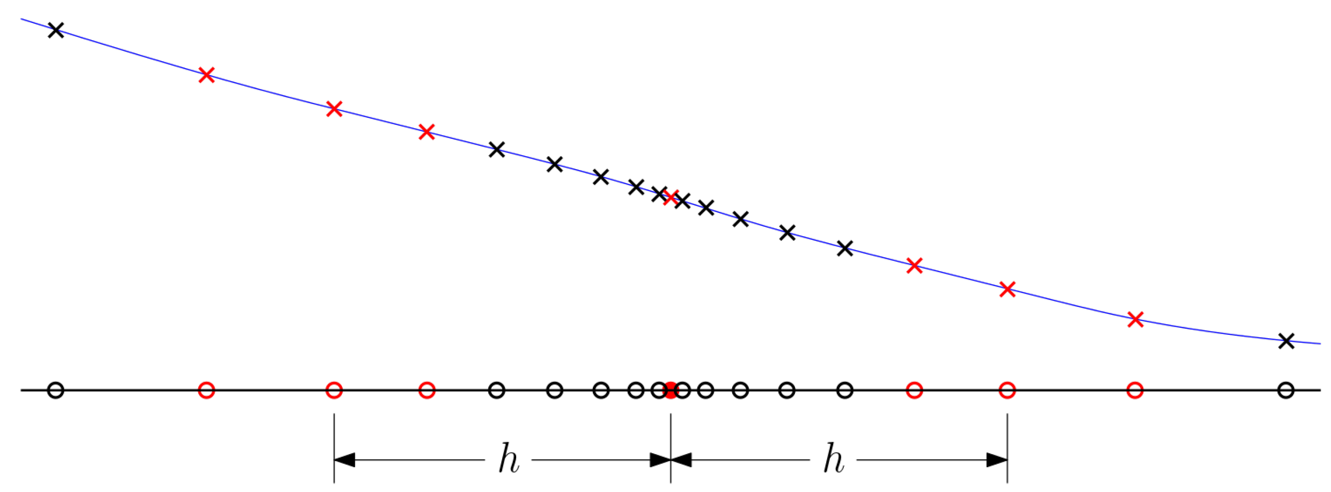
The gradient analysis is based on a centered parameter study within the design space. The study is centered around a given point, in this case, the solution given for the optimization problem (These methods can also be used to tune the gradients before an optimization, in this case, the centered parameter study would be focused around the initial design). Along the ordinates, the model is sampled with geometric spacing (i.e., increasing step length) to generate a set of points (i.e., $(x_1,y_1),(x_2,y_2),\dots ,(x_m,y_m)$, where x is a design variable and y is a response). This is sufficient to give all the finite difference estimates given in Equation (3). The polynomials were fit to the same data as well and all polynomials included the central point and two groups of points on either side of the central point. The step length associated with a given polynomial is based on the central point within these two side groups. Figure 2 gives an example of how 7 points can be used for a polynomial curve associated with a step length of h.

The polynomial regression is based on selecting m points as shown in Figure 2. An $n\mathrm{th}$-order polynomials shown in Equation (4) are fit to the data by solving Equation (5), where $n<(m+1)$. It is important to ensure that the polynomial fit is over-determined (i.e., fitting to more points than polynomial order) to quantify the quality of the fit and, subsequently, the gradient quality. In this work, linear, quadratic, and cubic polynomials were fit with 7, 9, and 11 points to give 9 polynomials in total for each step-size. These polynomial curves are shown as thin brown lines, along with the finite difference gradients in Figure 1.

$$y_i\approx f\left(x_i\right)=P_0+P_1{x}_i+P_2{x}_i^2+\dots +P_n{x}_i^n$$

(4)

$$\left[\begin{array}{cccc}{\displaystyle \sum _1^m}1& {\displaystyle \sum _1^m}{x}_i& \cdots & {\displaystyle \sum _1^m}{x}_i^n\\ {\displaystyle \sum _1^m}{x}_i& {\displaystyle \sum _1^m}{x}_i^2& \cdots & {\displaystyle \sum _1^m}{x}_i^{n+1}\\ ⋮& ⋮& \ddots & ⋮\\ {\displaystyle \sum _1^m}{x}_i^n& {\displaystyle \sum _1^m}{x}_i^{n+1}& \cdots & {\displaystyle \sum _1^m}{x}_i^{2n}\end{array}\right]\left[\begin{array}{c}{P}_0\\ P_1\\ ⋮\\ P_n\end{array}\right]=\left[\begin{array}{c}{\displaystyle \sum _1^m}{y}_i\\ {\displaystyle \sum _1^m}{y}_i{x}_i\\ ⋮\\ {\displaystyle \sum _1^m}{y}_i{x}_i^n\end{array}\right]$$

(5)

The coefficient of determination, defined in Equation (6), can be interpreted as the amount of variance in the samples that are captured by the fitted polynomial. As $R^2$ approaches 1, the polynomial fit can predict all the variance; when it reaches 1, the polynomial is a perfect fit passing through all the sample points. Figure 3 shows an example of the $1-\overline{R^2}$, which is based on the average coefficient of determination (For every step size, 9 separate polynomial curve fits were generated, along with 9 corresponding coefficients of determination. Instead of plotting all 9 coefficients of determination, we give the mean and standard deviation of these estimates in the plot.) over all the polynomial fits a given step size, along with the estimated gradients. Figure 3a shows that the best agreement between gradient estimates is achieved around a step size of 0.0001. Similarly, Figure 3b indicates the best quality-of-fit around the same step size. Furthermore, as the disagreement between estimates grows over the other step sizes in Figure 3a, we also see that the coefficient of determination statistics deteriorates at the corresponding step sizes in Figure 3b. For the sake of brevity, we only show one comparison between the gradient estimates and coefficient-of-determination. However, this work reviewed all the available data to ensure that the coefficient of the determinant was a robust measure for predicting good agreement between numerical gradients.

$$R^2=1-\frac{\sum {\left(y_i-f\left(x_i\right)\right)}^2}{\sum {\left(y_i-\overline{y}\right)}^2}$$

(6)

Assuming that the agreement between numerical gradient estimates corresponds to accurate gradients, we can then assume that gradient accuracy also corresponds to high values for the coefficient of determination. Thus, the optimal step size can be selected based on the step size that produces the maximum coefficient of determination (or minimum $1-\overline{R^2}$). Figure 3 shows that the standard deviation of the coefficient determination can also predict gradient quality. Furthermore, the blue curve combines both the mean and standard deviation of $R^2$ to give a hybrid measure of gradient quality.

Once the optimal step size is identified, the gradient can be estimated by a number of methods (It should be noted that each term in the Jacobian (i.e., unique pair of input and output scalar) has its own unique optimal step size. This has implications in tuning the gradients for finite difference as, at best, one selects only one step size for each input. However, if the different outputs give better gradients at different step sizes, the error is introduced using a single fixed step size. This error can only be eliminated by evaluating the gradients for each input over a range of step sizes.). In the POSA performed in this work, we assumed that the average over all the gradient estimates (At any given step-size, there is an estimate for each finite difference formula, along with the different estimates from each of the polynomial curve fits) at the optimal step size is the best available estimate for the gradient value. This best overall estimated gradient value was used to compute the Lagrange multipliers and perform the post-optimum sensitivity analysis in Section 4.2 and Section 5, respectively.

It is not practical to use the same type of best overall gradient estimate within an optimization as it is based on approximately 100 samples per design variable. The computational requirements of this calculation are of the same order of magnitude as the original optimization itself with simple first-order finite difference gradients. Instead, the results of this analysis should be used to tune standard finite difference methods.

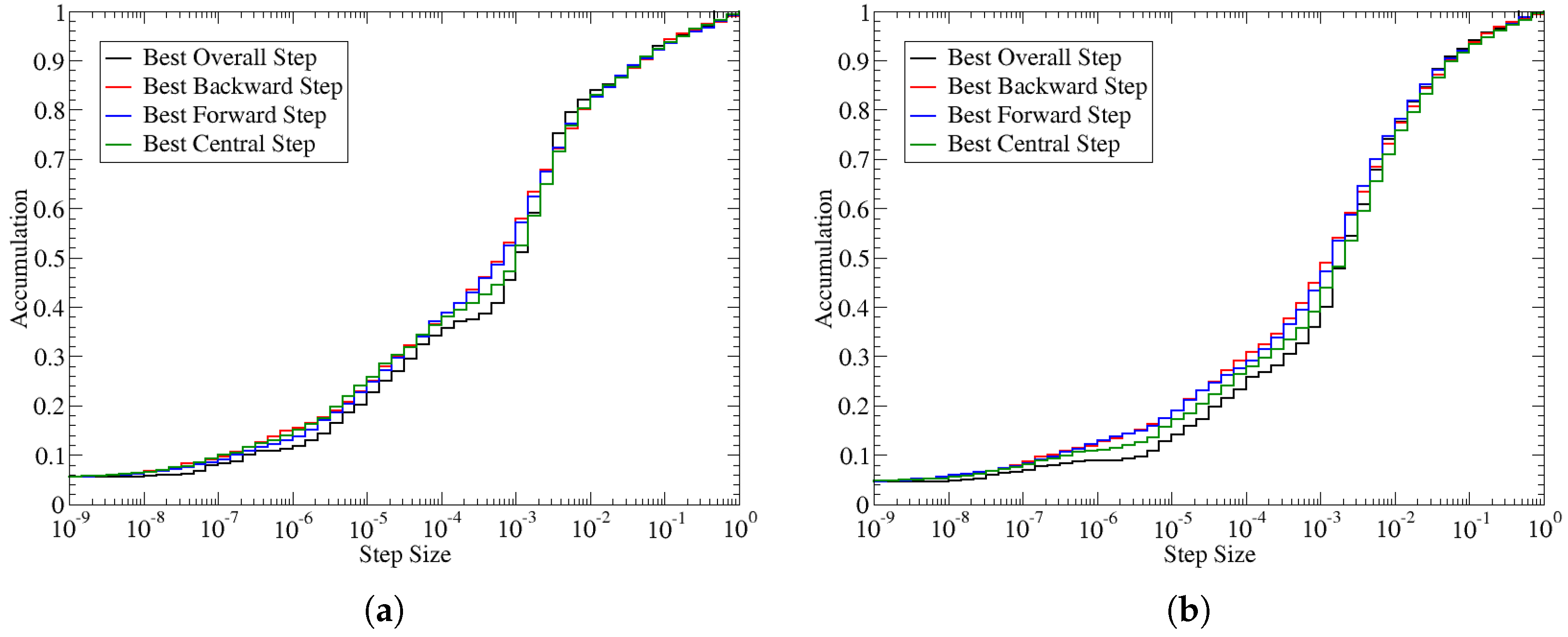
The coefficient of determination can be used to determine the best step size to take for each term in the Jacobian. As stated earlier, the optimal step size can be identified by the step-size that produces the smallest value for $1-mean\left(R^2\right)+stdev\left(R^2\right)$. Using this metric, we can collect an optimal step size for every term in the Jacobian. The statistics of the best step size are shown in the cumulative distribution in Figure 4. The frequency has been normalized such that a value of 1 represents all the available values. These statistics are based on selecting the best step size for each term within the Jacobian. However, within an optimization, only a single step size can be selected; according to the figure, a step size between 0.001 and 0.002 would represent the best compromise as an equal number of Jacobian terms would be optimal at either smaller or larger step values. Since the best step for an individual term is not necessarily consistent across all Jacobian terms, there is additional gradient error due to the spread in the optimal step size. The graph also shows that there is a wide variation in the optimal step size, suggesting that the error by selecting only a single step size could potentially be quite high.

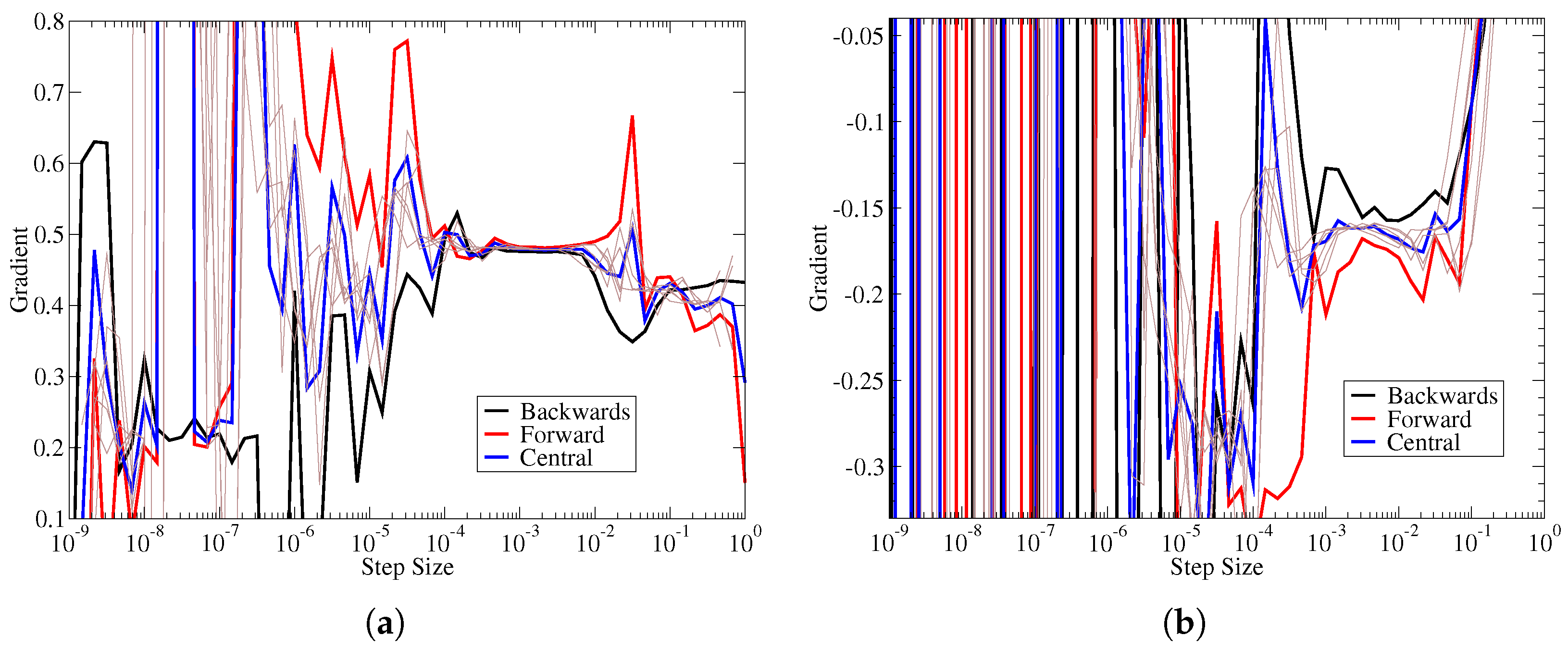
The coefficient of determination statistics also provides a measure of quality for the gradients. The quality measure used here was $1-mean\left(R^2\right)+stdev\left(R^2\right)$. Lower values of this measure reflect better quality gradients, as shown in Figure 3. For each input/output pair in the Jacobian, there was a minimum value achieved for the quality measure over all the step sizes. If that minimum value was quite small, it reflects that there is a step size where there is a high degree of agreement between the gradient estimates. Figure 5a shows that when the floor of the quality measure reaches $1\times {10}^{-5}$, there is a region with very good agreement between estimates. For the data in Figure 5a, it is achieved at around a step size of 0.002. However, if the floor of this quality measure for a given input/output pair cannot reach such small values, then the best agreement between numerical gradients is also worse. Figure 5b shows an example of gradient estimates when the quality measure reached a minimum of $1\times {10}^{-3}$ at a step size of 0.002. In Figure 5b there is approximately a $10\%$ difference between the gradients. For the sake of brevity, this paper only shows a couple of examples, however, this correspondence between best quality measurement and the degree of agreement between gradient estimates was consistent throughout all the data. Thus, one can estimate the overall gradient quality based on statistics of the quality measure. Our work shows that quality measure of $1\times {10}^{-3}$ likely contains some error, but should give acceptable results, while one should try to achieve a quality measure closer to $1\times {10}^{-5}$.

4. Post-Optimum Sensitivity Analysis

For the optimization problem in Equation (7), where $\mathit{x}$ contains the design variables, ${\mathit{x}}_l$ and ${\mathit{x}}_u$ are the lower and upper bounds on the design variables, $f(\mathit{x},\mathit{p})$ is the objective, $\mathit{g}(\mathit{x},\mathit{p})$ represents the inequality constraints and $\mathit{h}(\mathit{x},\mathit{p})$ the equality constraints. Similarly, ${\mathit{g}}_l$ and ${\mathit{h}}_l$ corresponding to the limit values for the inequality and equality constraints respectively. Finally, $\mathit{p}$ are the parameters that are held constant within the optimization, but could be varied in the larger design process.

$$\begin{array}{cc}\hfill \underset{\mathit{x}}{min}& f(\mathit{x},\mathit{p})\hfill \\ \hfill \mathrm{such}\mathrm{that}& \mathit{x}\ge {\mathit{x}}_l\hfill \\ \hfill & \mathit{x}\le {\mathit{x}}_u\hfill \\ \hfill & \mathit{g}(\mathit{x},\mathit{p})-{\mathit{g}}_l<\mathbf{0}\hfill \\ \hfill & \mathit{h}(\mathit{x},\mathit{p})-{\mathit{h}}_l=\mathbf{0}\hfill \end{array}$$

(7)

The KKT conditions [29] are given in Equations (8) to (18), where ${\mathbf{\mu }}_i$, ${\mathbf{\mu }}_e$, ${\mathbf{\mu }}_l$ and ${\mathbf{\mu }}_u$ are the Lagrange multipliers for the inequality, equality, lower bound and upper bound constraints respectively. Equation (8) is the stationary condition, Equations (9) to (12) are the primal feasibility conditions, Equations (13) to (15) are the dual feasibility conditions and Equations (16) to (18) are the complimentary conditions.

$$\nabla f(\mathit{x},\mathit{p})+{\left[\nabla \mathit{g}(\mathit{x},\mathit{p})\right]}^T{\mathbf{\mu }}_i+{\left[\nabla \mathit{h}(\mathit{x},\mathit{p})\right]}^T{\mathbf{\mu }}_e-\mathit{I}{\mathbf{\mu }}_l+\mathit{I}{\mathbf{\mu }}_u=\mathbf{0}$$

(8)

$$\mathit{x}\ge {\mathit{x}}_l$$

(9)

$$\mathit{x}\le {\mathit{x}}_u$$

(10)

$$\mathit{g}(\mathit{x},\mathit{p})-{\mathit{g}}_l<0$$

(11)

$$\mathit{h}(\mathit{x},\mathit{p})-{\mathit{h}}_l=0$$

(12)

$${\mathbf{\mu }}_l\ge 0$$

(13)

$${\mathbf{\mu }}_u\ge 0$$

(14)

$${\mathbf{\mu }}_i\ge 0$$

(15)

$${\mathbf{\mu }}_l^T({\mathit{x}}_l-\mathit{x})=0$$

(16)

$${\mathbf{\mu }}_u^T(\mathit{x}-{\mathit{x}}_u)=0$$

(17)

$${\mathbf{\mu }}_i^T(\mathit{g}(\mathit{x},\mathit{p})-{\mathit{g}}_l)=0$$

(18)

The primal feasibility conditions are true for any feasible design point and valid optimization solution. The consequence of the complimentary conditions is that the Lagrange multipliers for inactive inequality constraints are zero and do not need to be calculated. Finally, the dual feasibility conditions become important in estimating the Lagrange multipliers, as they serve as a constraint on valid values.

In engineering design, one may want to improve the design beyond the optimal solution. To achieve this, innovation is required to relax some of the constraints, for example a strength constraint can be overcome by using better materials. To improve the design in this way, the question arises: what constraints have the strongest impact on the design? Each of the constraints has two parts: one part that is a function of the design variables and a second part that is a constant corresponding to the limit. The Lagrange multipliers can then be interpreted as how the objective would change, with changes in the constraint limit [30]. Thus, the the Lagrange multipliers are a sensitivity of the optimal design performance with respect to the design limits.

The design also depends on a variety of parameters that do not represent design variables or constraint limits. Examples may include material properties, environmental parameters, airfoil polar data, and more. These parameters also reflect additional paths to improving the design. To include them into the post-optimal sensitivity analysis, these parameters should be treated as design variables in the sensitivity analysis, then constrained by equality constraints of the following form: ${\mathit{x}}_p-\mathit{p}=0$ [30]. The design variable ${\mathit{x}}_p$ is used in place of the parameters, while the constant $\mathit{p}$ takes the value that was used in the optimization. The Lagrange multipliers corresponding to these additional equality constraints reflect how the design would improve with changes in these parameters [30].

4.1. Determining the Active Set

The first step in estimating these Lagrange multipliers is to identify the active set. In this work, any constraint value within ${10}^{-3}$ of the limit was considered active. A vast majority of the active constraints were geometric constraints to avoid degenerate designs (e.g., negative thickness, minimum widths, etc.). These simple geometric constraints were included in the analysis, but excluded from the presentation. Since the optimization did not perfectly converge, additional constraints of interest were included if they were within 10%. These include the constraints that are typically driving the design like tip deflection or blade root flap-wise bending moments.

A consequence of including a large number of geometric constraints was that it introduced a lot of redundancy into the active set. To improve the analysis, a pre-processing step was carried out to filter out these redundant constraints. Figure 6 shows an example of redundant inequality constraints. The constraint boundaries are represented by lines, where the lines within the infeasible set are redundant since the optimization would be constrained before the redundant constraints would become active. Another consideration shown in the figure is that two active constraints can still span the same vector space but not be redundant if they happen to point in opposite directions. This is a consequence of the dual feasibility conditions.

The algorithm to filter redundant constraints starts by initializing the active set of constraints that we want to prioritize in the analysis. These include equality constraints that are always active and inequality constraints that we know are important for blade design (e.g., blade root flap-wise bending moment, tip deflection). Then the remaining constraints are sorted according to the distance to the constraint limit with increasing distance. Then in this order, each constraint is tested to determine whether it is redundant or not. If the constraint is not redundant, then the constraint is added to the active set. All subsequent tests will also test against this added constraint. By performing this test in order of increasing distance, we assume that any redundant constraint is already behind the constraint boundaries of active constraints and not active.

With this assumption in hand, we can identify the redundant constraints according to the angles with respect to the remaining constraints. If the angle between a candidate constraint and the current set of active constraints is less than a specified threshold; then it could be assumed that the candidate constraint is redundant and rejects it from the active set. The angle between two vectors can be calculated as shown in Equation (19), where vectors $\mathit{w}$ and $\mathit{x}$ are two arbitrary vectors.

$$\theta =arccos\left(\frac{\mathit{w}\times \mathit{x}}{{\parallel \mathit{w}\parallel }_2{\parallel \mathit{x}\parallel }_2}\right)$$

(19)

Following this definition, we can determine the angle between vector spaces. A vector space can be represented as a matrix of vectors ($\mathit{W}$), a Singular Value Decomposition (SVD) of that matrix can then be taken according to Equation (20). The properties of the SVD are that $\mathit{U}$ and ${\mathit{V}}^T$ define an orthonormal basis such that ${\mathit{U}}^T\mathit{U}=\mathit{I}$ and $\mathit{V}{\mathit{V}}^T=\mathit{I}$. Furthermore, the matrix $\mathit{S}$ is a diagonal matrix of singular values. The singular values are non-negative numbers, where the value 0 typically corresponds to the null space of the original matrix. The second definition in Equation (20) shows the SVD partitioned such that all the non-zero singular values are in ${\mathit{S}}_{w1}$ and the null space corresponds to the matrices ${\mathit{U}}_{w2}$ and ${\mathit{V}}_{w2}^T$.

$$\begin{array}{cc}\hfill \mathit{W}& ={\mathit{U}}_w{\mathit{S}}_w{\mathit{V}}_w^T\hfill \\ \hfill & =\left[\begin{array}{cc}{\mathit{U}}_{w1}& {\mathit{U}}_{w2}\end{array}\right]\left[\begin{array}{cc}{\mathit{S}}_{w1}& \mathbf{0}\\ \mathbf{0}& {\mathit{S}}_{w2}\end{array}\right]\left[\begin{array}{c}{\mathit{V}}_{w1}^T\\ {\mathit{V}}_{w2}^T\end{array}\right]\hfill \end{array}$$

(20)

The angle of the vector space $\mathit{X}$ against the vector space $\mathit{W}$ can be calculated by projecting $\mathit{X}$ onto the null space of $\mathit{W}$. This is shown in Equation (21).

$$\mathit{O}={\mathit{V}}_{x1}^T{\mathit{V}}_{w2}{\mathit{V}}_{w2}^T$$

(21)

It is then useful to determine the dominant directions of $\mathit{O}$ to find directions that have the largest angle against $\mathit{W}$. This can be identified by performing a SVD on $\mathit{O}$, by convention the singular values are sorted in decreasing order. Thus, the largest angle corresponds to the first singular value according to Equation (22) following by the next largest angle and so forth. When the vector space $\mathit{X}$ only contains a single vector, then there is only one angle between this vector and the vector space $\mathit{W}$.

$${\theta }_i=arcsin\left(S_{Oi}\right)$$

(22)

As the dual feasibility conditions do not apply to the equality constraints, we can use the definition in Equation (22) to define the angle between a candidate and the equality constraints.

For the inequality constraints within the active set, we need to consider that two parallel constraints pointing in opposite directions are not redundant. As the definition in Equation (22) ignores this dependence on direction, it cannot be used to test the angle against a set of inequality constraints. Instead the degree to which the active set can span a candidate vector can be determined by solving the optimization problem in (23), where $\mathit{W}$ is the active set, $\mathit{w}$ are a set of weights and $\mathit{x}$ is the candidate vector.

$$\begin{array}{cc}\hfill \underset{\mathit{w}}{min}& {\parallel \mathit{W}\mathit{w}-\mathit{x}\parallel }_2\hfill \\ \hfill \mathrm{s}.\mathrm{t}.& \mathit{w}\ge 0\hfill \end{array}$$

(23)

As there are small errors in $\mathit{W}$, it is helpful to condition the problem with a SVD and to normalize $\mathit{x}$ (denoted by $\widehat{\mathit{x}}$). This leads to the quadratic programming problem in Equation (24).

$$\begin{array}{cc}\hfill \underset{\mathit{x}}{min}& \frac{1}{2}{\mathit{w}}^T{\mathit{U}}_{w1}{\mathit{S}}_{w1}{\mathit{S}}_{w1}^T{\mathit{U}}_{w1}^T\mathit{w}-{\mathit{w}}^T{\mathit{U}}_{w1}{\mathit{S}}_{w1}{\mathit{V}}_{w1}^T\widehat{\mathit{x}}\hfill \\ \hfill \mathrm{s}.\mathrm{t}.& \mathit{w}\ge 0\hfill \end{array}$$

(24)

The optimal solution to Equation (24) is given as ${\mathit{w}}^{*}$, with this solution, the angle a candidate vector take against a set of inequality constraints can be defined as shown in Equation (25).

$${\theta }_i=arcsin\left(\parallel {\mathit{w}}^{*T}{\mathit{U}}_{w1}{\mathit{S}}_{w1}{\mathit{V}}_{w1}^T{-\mathit{x}\parallel }_2\right)$$

(25)

4.2. Estimating the Lagrange Multipliers

Estimating the Lagrange multipliers is based on minimizing the stationary conditions (i.e., Equation (8)), subject to the dual feasibility conditions (i.e., Equations (13) to (15)). This can be achieved in two steps. First, a set of Lagrange multipliers that minimize the stationary conditions is obtained by solving the quadratic programming problem in Equation (26).

$$\begin{array}{cc}\hfill \underset{{\mathbf{\mu }}_i,{\mathbf{\mu }}_e,{\mathbf{\mu }}_l,{\mathbf{\mu }}_u}{min}& \frac{1}{2}\left\{\begin{array}{cccc}{\mathbf{\mu }}_i& {\mathbf{\mu }}_e& {\mathbf{\mu }}_l& {\mathbf{\mu }}_u\end{array}\right\}\mathit{G}{\mathit{G}}^T\left\{\begin{array}{c}{\mathbf{\mu }}_i\\ {\mathbf{\mu }}_e\\ {\mathbf{\mu }}_l\\ {\mathbf{\mu }}_u\end{array}\right\}\hfill \\ \hfill & -\left\{\begin{array}{cccc}{\mathbf{\mu }}_i& {\mathbf{\mu }}_e& {\mathbf{\mu }}_l& {\mathbf{\mu }}_u\end{array}\right\}\mathit{G}\mathbf{\nabla }f(\mathit{x},\mathit{p})\hfill \\ \hfill \mathrm{s}.\mathrm{t}.& {\mathbf{\mu }}_i\ge \mathbf{0}\hfill \\ \hfill & {\mathbf{\mu }}_l\ge \mathbf{0}\hfill \\ \hfill & {\mathbf{\mu }}_u\ge \mathbf{0}\hfill \end{array}$$

(26)

The overall active constraint Jacobian ($\mathit{G}$) is defined by the Jacobians of the active constraints (denoted with a subscript ${•}_a$) as shown in Equation (27).

$$\mathit{G}=\left[\begin{array}{c}\mathbf{\nabla }{\mathit{g}}_a(\mathit{x},\mathit{p})\\ \mathbf{\nabla }{\mathit{h}}_a(\mathit{x},\mathit{p})\\ -{\mathit{I}}_a\\ {\mathit{I}}_a\end{array}\right]$$

(27)

The solution to Equation (26) is denoted by ${\mathbf{\mu }}_i^{+}$, ${\mathbf{\mu }}_e^{+}$, ${\mathbf{\mu }}_l^{+}$ and ${\mathbf{\mu }}_u^{+}$. This solution is not unique due to a null space over the constraint matrices. To make the solution unique, a second quadratic programming problem, shown in Equation (28), is solved to obtain the final set of Lagrange multipliers. This optimization problem is based on minimizing the magnitude of the Lagrange multipliers, the equality constraint ensures that the final solution is still a solution the minimizes the problem in Equation (26).

$$\begin{array}{cc}\hfill \underset{{\mathbf{\mu }}_i,{\mathbf{\mu }}_e,{\mathbf{\mu }}_l,{\mathbf{\mu }}_u}{min}& \frac{1}{2}\left\{\begin{array}{cccc}{\mathbf{\mu }}_i& {\mathbf{\mu }}_e& {\mathbf{\mu }}_l& {\mathbf{\mu }}_u\end{array}\right\}\left\{\begin{array}{c}{\mathbf{\mu }}_i\\ {\mathbf{\mu }}_e\\ {\mathbf{\mu }}_l\\ {\mathbf{\mu }}_u\end{array}\right\}\hfill \\ \hfill \mathrm{s}.\mathrm{t}.& {\mathbf{\mu }}_i\ge \mathbf{0}\hfill \\ \hfill & {\mathbf{\mu }}_l\ge \mathbf{0}\hfill \\ \hfill & {\mathbf{\mu }}_u\ge \mathbf{0}\hfill \\ \hfill & \mathit{G}\left\{\begin{array}{c}{\mathbf{\mu }}_i\\ {\mathbf{\mu }}_e\\ {\mathbf{\mu }}_l\\ {\mathbf{\mu }}_u\end{array}\right\}=\mathit{G}\left\{\begin{array}{c}{\mathbf{\mu }}_i^{+}\\ {\mathbf{\mu }}_e^{+}\\ {\mathbf{\mu }}_l^{+}\\ {\mathbf{\mu }}_u^{+}\end{array}\right\}\hfill \end{array}$$

(28)

5. Post-Optimal Sensitivity Study

A post-optimal sensitivity study looks at the Lagrange multipliers to determine the dominate constraints that are driving the design. The values taken directly from the optimization are not comparable, due to the different units of the different constraint equations. To compare the Lagrange multipliers, they are normalized by the constraint limit and the optimal objective value (i.e., AEP) as shown in Equation (29), where ${\mu }_i$ denotes a single Lagrange multiplier and $g_{li}$ the corresponding constraint limit and finally $f^{*}$ the optimal objective value. When normalized, the Lagrange multiplier can be interpreted as the relative improvement in objective with respect to relative change in the constraint limit. So a normalized Lagrange multiplier of 0.1 implies that if the constraint limit was increased by 10%, the AEP would improve by 1%.

$${\tilde{\mu }}_i=\frac{g_{li}{\mu }_i}{f^{*}}$$

(29)

The post-sensitivity analysis is given here in three sections. First, the Lagrange multipliers for the standard load constraints in the standard optimization problem are given in Section 5.1. Second, the Lagrange multipliers associated with selected parameters is given in Section 5.2. Finally, this work looked at how the optimal design itself would change by varying constraint limits and parameters in Section 5.3.

5.1. Sensitivity to Standard Load Constraints

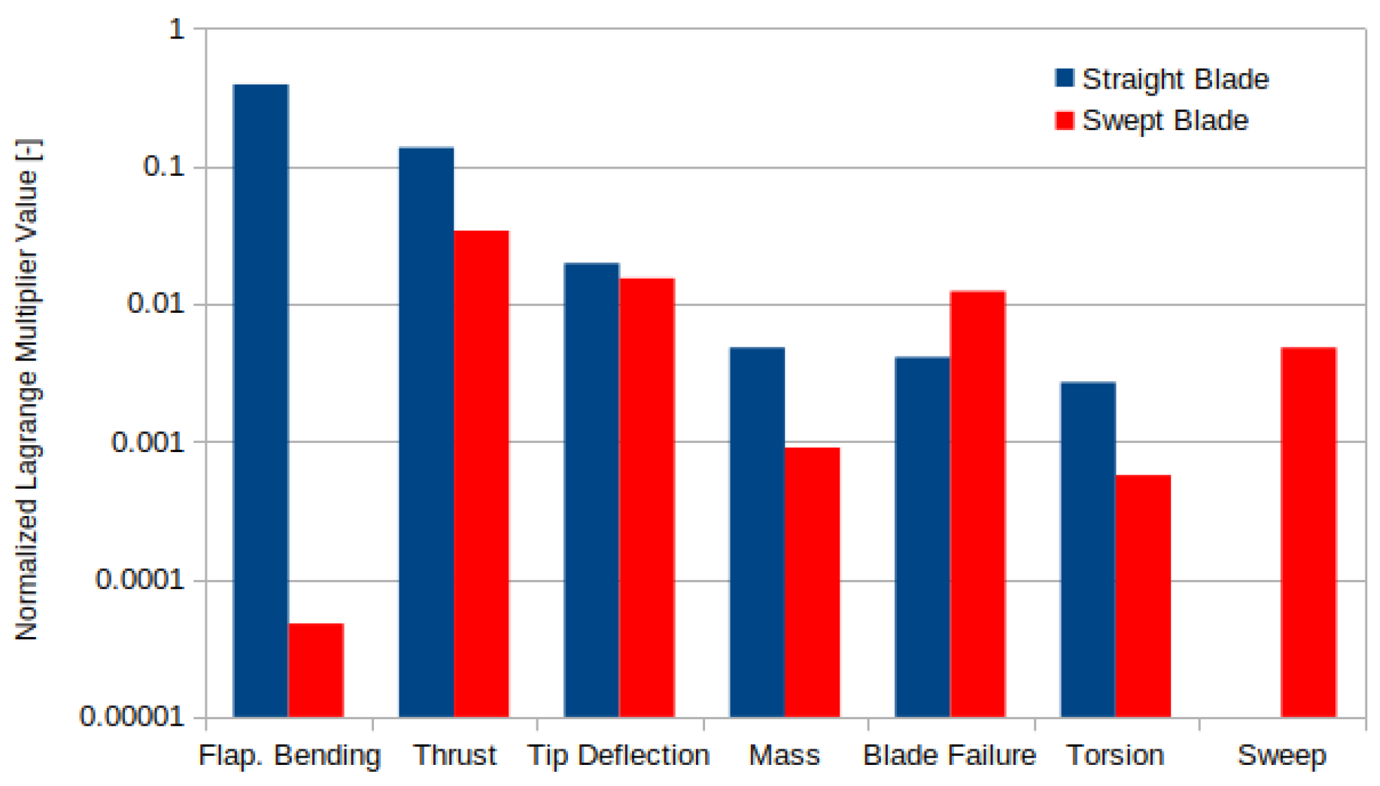
Figure 7 shows the Lagrange multipliers associated with the selected constraints. First, the straight blade Lagrange multipliers show that the conventional blade design is highly sensitive to the typical limiting load constraints. The design is dominated by blade root flap-wise bending moment, followed by thrust. The sensitivity to blade root flap-wise bending moment is expected since extending the blade both increases the thrust and the moment arm, while the limit on thrust indirectly limits the power (i.e., $P=TV$). Next the design is sensitive to tip deflection by an order of magnitude less than the load constraints, the reduced sensitivity to tip deflection is due to increased design freedom in controlling deflection (i.e., pre-bend and stiffness). The straight blade is still sensitive to blade failure and blade root torsion moment, but significantly less than the other constraints.

The swept blade results showed similar Lagrange multipliers as the straight blade, except that there is significantly less sensitivity in the blade root flap-wise bending moment constraint. This is due to the fact that the sweep reduces the loading at the outboard sections of the blade and thus reduces the bending moment. Furthermore, the increased design freedom of sweep shows that the design is moderately less sensitive to the remaining load constraints. However, since the load alleviation relies on blade deformation the design becomes increasingly more sensitive to material failure. The optimization did not include a cost model, so the mass constraint was added to avoid significant increases in the cost. The smaller Lagrange multipliers for this constraint in the swept blade optimization suggest that swept blades could be cheaper than conventional blades. Finally, the Lagrange multiplier on the sweep constraint is significant, suggesting that further improvement could be achieved if the blade was allowed to sweep more.

5.2. Sensitivity to Parameters

To gain further insights into the impact of sweep on the design problem, the post-optimum sensitivity study was extended to include important parameters. These parameters are included in the Lagrange multiplier estimation by introducing them as design variables and then using equality constraints to fix them to their nominal values. This creates the extended problem in Equation (30), where ${\mathit{p}}_c$ are the constant parameter values that were used to solve Equation (7). Equation (30) does not need to be solved because solutions to Equation (7) are still solutions to Equation (30). This extended problem gives insights into the impact of parameters by estimating the Lagrange multipliers associated with the equality constraints on the parameter values. Like other constraints, this shows how the objective will change with respect to changes in the parameter value.

$$\begin{array}{cc}\hfill \underset{\mathit{x},\mathit{p}}{min}& f(\mathit{x},\mathit{p})\hfill \\ \hfill \mathrm{s}.\mathrm{t}.& \mathit{x}\ge {\mathit{x}}_l\hfill \\ \hfill & \mathit{x}\le {\mathit{x}}_u\hfill \\ \hfill & \mathit{g}(\mathit{x},\mathit{p})-{\mathit{g}}_l<\mathbf{0}\hfill \\ \hfill & \mathit{h}(\mathit{x},\mathit{p})-{\mathit{h}}_l=\mathbf{0}\hfill \\ \hfill & \mathit{p}-{\mathit{p}}_c=\mathbf{0}\hfill \end{array}$$

(30)

The optimization problem here was extended with the material stiffness and failure properties were investigated to determine the influence of material selection. The optimization included a deterministic gust to simulate the effect of unsteady flow, the magnitude of this gust was also considered as an important parameter. The sensitivity to the gust magnitude should reflect a sensitivity to turbulence.

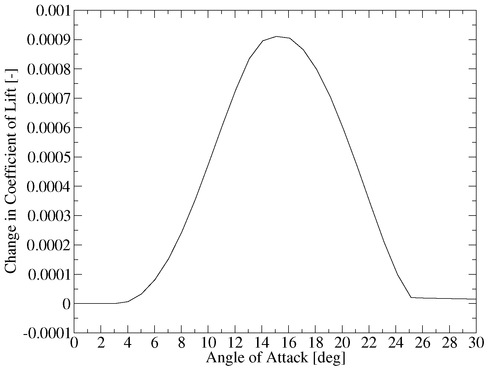
To explore the impact of detailed aerodynamic design, a synthetic airfoil polar generator was developed to model realistic improvements in lift and drag. Improvement in lift is parameterized as an improvement in the $C_l$ max by adding the perturbation function shown in Figure 8 to alter the $C_l$. The magnitude of the perturbation shown in Figure 8 gave the best quality gradients in this study. The improvement in drag was simulated by simply changing all the drag values accordingly.

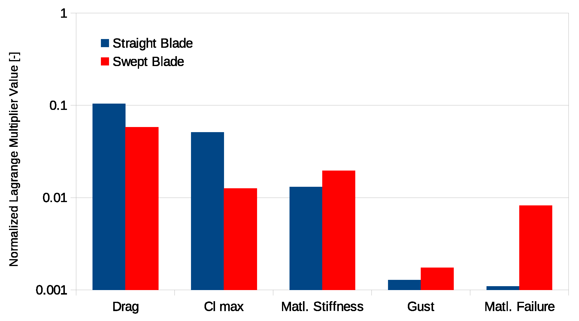
Figure 9 shows the Lagrange multipliers associated with the different parameters in the optimization. The parameters explored here look at the impact of cross section aerodynamics and material properties. The optimization did not simulate the impact of turbulence, instead a deterministic gust was used in-place of turbulence.

For conventional blade design, the cross section aerodynamics have a larger impact on the design than the material properties. This is because power is directly dependent on aerodynamic forces, whereas material properties have a less direct dependency on the power. However, in a swept blade design, blade deformation is utilized to reduce loads. In this case, the aerodynamic properties matter less and the material properties start to have equal importance as the aerodynamics. In both cases the optimization has low sensitivity to the gust parameter. Yet, in conventional blade design, turbulence levels have a strong influence on the loads. So this low sensitivity indicates that a gust does not fully capture effects of turbulence on blade design.

5.3. Impact of Relaxing Constraints on the Design

The first part of the post-optimal sensitivity quantified how the performance would improve if a given constraint was relaxed. This section provides an estimate to the changes in the design variables that would achieve the improvement if a given constraint was relaxed. This could be determined accurately by solving Equation (7) several times with different constraints relaxed. This approach is not attractive due to the cost of solving this problem for each constraint. Instead, this section acquires these estimates based on the gradient information alone without solving the optimization problem.

Castillo et al. [30] demonstrates how the KKT conditions can be used to estimate how the design variables would change with respect to changes in the various constraints and parameters. This analysis requires second order gradient information, which for the tools used here can only be calculated by finite difference. These second order gradients are significantly more expensive and more sensitive to numerical errors than the first order gradients. Instead, this research developed a different approach using only first order gradients. (Note, that an attempt was made by casting the problem as a linear programming problem using only the first order gradient information. Another attempt was made by solving a pseudo inverse of the stationary conditions of the KKT conditions. In both cases, the solution is highly sensitive to small numerical errors. These problems can be mitigated by pre-conditioning the constraint Jacobians, however, the solution was also sensitive to this pre-conditioning as well. So in the absence of accurate gradients a different approach is needed.)

The approached developed here is a geometric approach, that tries to determine how the set of feasible directions would change when constraints are relaxed. This is determined by the Jacobians of the active constraints as explained in Section 4.1. The active set is further reduced by rejecting constraints associated with Lagrange multipliers values approaching zero. For each relaxed constraint in consideration, this constraint Jacobian is partitioned into a Jacobian for the relaxed constraint (${\mathit{G}}_i$) and a constraint Jacobian without the relaxed constraint (${\mathit{G}}_{\backslash i}$). The assumption is that the design will change within the span of ${\mathit{G}}_i$ that is orthogonal to ${\mathit{G}}_{\backslash i}$. This space is defined by the span of ${\mathit{P}}_i$ defined in Equation (31), where ${\mathit{S}}_i$ is the span of ${\mathit{G}}_i$ and ${\mathit{N}}_{\backslash i}$ is the null space of ${\mathit{G}}_{\backslash i}$.

$${\mathit{P}}_i={\mathit{N}}_{\backslash i}{\mathit{N}}_{\backslash i}^T{\mathit{S}}_i$$

(31)

Then the direction the design would change is given by Equation (32) where ${\mathit{S}}_{pi}$ is the orthonormal span of ${\mathit{P}}_i$.

$$\mathit{q}=-{\mathit{S}}_{pi}{\mathit{S}}_{pi}^T\mathbf{\nabla }f(\mathit{x},\mathit{p})$$

(32)

The direction given in Equation (32) is only a direction and does not accurately show in magnitude how the design variables would change with respect to unit changes in the constraint limits. This rate could be estimated by multiplying $\mathit{q}$ by $\frac{\lambda }{\mathit{q}\times \mathbf{\nabla }f}$. Since $\mathit{q}$ and $\mathbf{\nabla }f$ are nearly orthogonal in most cases, this scaling is poorly conditioned and was not applied. Instead the design vector $\mathit{q}$ is normalized to have a unit length so the results show relatively what design variables are most sensitive to the different constraint limits.

Changes in the Design Due to Relaxed Constraints

Investigating the impact of relaxing constraints on the design itself generates a large amount of data; thus, we presented only the most interesting aspects of this work. Additionally, the methods to determine these changes only gives the direction in the design vector at the limit. Thus, the designs that are presented here are not realistic designs that would be generated from a full optimization, but more a general direction the optimization would take if a given constraint was relaxed.

The design direction calculated in Equation (32) has an entry that corresponds to how the blade length would change if a given constraint was relaxed. Recall that this vector is normalized to unit magnitude, so the magnitude of this entry indicates the degree to which a given constraint is limiting the blade length. These results are shown in

Table 1. The Effect of Constraints on Blade Length.

Constraint	Straight Blade	Swept Blade
Pre-bend	0.462	0.032
Tip Deflection	0.285	0.182
Thrust	0.267	0.320
Torsion	0.175	0.212
Mass	0.127	0.250

, they show that for the straight blade, the blade length is most strongly limited by the allowed pre-bend and the tip-deflection constraint. However, for a swept blade, these constraints are less important, instead the thrust, blade root torsion moment, and mass play a larger role. This demonstrates that the bend-twist coupling can be utilized to attenuate the impact of tip deflection constraints.

These design direction vectors can also be used to show how distributed quantities like chord and twist would change if different constraints were relaxed. Each of the different directions, calculated with Equation (32) for each constraint, were normalized to have a unit length. Then the optimal design were perturbed according to this normalized direction to generate updated blade designs shown below.

First, the updated blade designs indicated that the sweep limit and the blade root torsion moment constraint had the largest influence on the sweep. Figure 10 shows the direction that the sweep distribution would change if these two constraints were relaxed independently. The red curve shows how the sweep would change if the sweep limit was increased, while the blue shows how the sweep would change if the blade root torsion moment constraint was relaxed. When the sweep limit is increased, the sweep is increased accordingly without a major change in the shape (see the red curve in Figure 10). When the torsion constraint is relaxed, the optimization moves towards including a combination of both forwards and backward sweeps to increase the overall moment arm at intermediate sections of the blade (see the blue curve in Figure 10). Both changes would increase the bend twist coupling effect, thus, confirming that the blade performance could be improved with increased sweep.

Table 1 indicates that the blade length is most affected by the thrust constraint. However, relaxing the thrust constraint would also change other design variables. One can use similar plots to investigate these additional changes, as shown in Figure 11. The plots show that the optimization would move to increase the chord. This would increase both the aerodynamic loading and the stiffness of the blade. To compensate for the increased aerodynamic loading, the twist is reduced by approximately $0.5^{\circ }$ overall. The increased stiffness allows the optimization to choose thinner airfoils that are more flexible but also more aerodynamically efficient. Since the plots are based on a single constraint being relaxed, the longer blade must still respect the same blade root flap-wise bending moment and tip deflection constraints. To achieve this, the optimization would introduce a combination of forward and backward sweeps to increase the bend twist coupling.

6. Conclusions

This research has developed a statistical technique for automatically tuning numerical gradients based on polynomial regression and the coefficient of determination. This research has demonstrated how this method can be used to tune the step size for conventional low order numerical gradients, determine the best overall estimate of the gradient values and evaluate the overall quality of the numerical gradients.

This paper has applied these accurate gradients in a POSA to understand how various constraints and parameters affect the performance and design of the optimal solution. Generally, a basic application of POSA depends on optimization algorithms that produce accurate Lagrange multipliers. In this case, only the sensitivity with respect to load constraints can be evaluated. The method developed in this paper does not rely on the optimization algorithm and thus can be applied to solutions obtained by any optimization algorithm (i.e., gradient-free methods). The method presented here extends the basic application of POSA to show how the optimal solution would change with respect to parameters. The method is further extended to show how the optimal design solution itself would change with respect to relaxed constraints or changes in the parameters. The advantage of POSA is that design engineers can determine what changes to the optimization problem and/or innovations that are required further to improve the optimal design without running multiple optimization calculations.

The method developed here was applied to an optimal straight and swept blade. The POSA showed that the conventional straight blade was strongly sensitive to blade root-flap-wise bending moment, thrust, and tip deflection. However, once the optimization can introduce sweep (i.e., load alleviation via bend-twist coupling), the blade root-flap-wise bending moment was no longer driving the design. Furthermore, the optimization can utilize bend-twist coupling further to reduce the impact of thrust and tip-deflection constraints. However, as the load alleviation relies on deformation, the swept blade design becomes more sensitive to material failure.

The POSA was extended to investigate the impact of selected parameters. In the conventional straight blade, the optimization is more sensitive to the airfoil design than the material properties. However, in the swept blade optimization, the sensitivity to aerodynamic parameters is reduced. While the sensitivity to material properties starts to have similar importance to the aerodynamic properties. This makes sense considering that the swept blade relies on deformation to achieve load alleviation.

The POSA was also applied to estimate how the design itself would change by relaxing selected load constraints. For conventional straight blade optimization, the length of the blade is most sensitive to the allowed pre-bend and tip deflection. However, when the sweep is introduced, the overall thrust, blade root torsion moment and mass start to have a larger influence on the blade length. The same analysis also showed that the maximum allowed sweep constraint and the maximum blade root torsion moment constraint were the strongest drivers for the sweep design. The analysis showed that the optimization would increase the bend-twist coupling effect if either of these constraints were relaxed. Thus, further design improvement can be achieved by increasing sweep. Finally, as the thrust had the greatest effect on blade length for the swept blade, the POSA was applied to understand how the planform design variables would change when the thrust constraint is relaxed. The results showed that the chord would increase, twist decrease, more flexible and aerodynamically efficient airfoils are selected, while bend-twist coupling is increased.

Overall, this paper has developed methods for improving the accuracy of numerical gradients, additional methods for POSA and applied these methods to a straight and swept blade optimization. The paper has demonstrated how POSA can reveal how different aspects of the optimization can be improved, thus guiding the overall design process. Without POSA, this information could only be obtained by running multiple optimizations and thus very expensive. Hence the value of these contributions is increased information on the design without the computational burden of multiple optimizations.