1. Introduction
The electric power industry has been subject to constant changes. Utility companies have been aware of the threats and opportunities that arise as a result of this change. Climate action calls for the electric power industry to participate in the energy transition, once it is an important player in integrating more variable renewable energy sources and guaranteeing energy distribution for new needs, such as charging electrical vehicles, green hydrogen production, industrial heating electrification, and other opportunities for electrification all supported by renewable energy. The growing popularity of “behind the meter” on-site generation and storage, the new digital retail competitors that serve customers with bundle solutions towards energy-as-a-service business models, increased search for grid flexibility, and intense public and regulatory scrutiny are just some strengths that reinforce the need for more digitalization in the energy sector [
1,
2,
3,
4].
Data are an important asset that utilities have available today to support management decisions, excel in operational efficiency, and be more competitive. Moreover, data and technology to extract value from these data, generally addressed by artificial intelligence and machine learning, are no longer just a technological enabler, but rather an integrated part of the acceleration of the energy transition. The complex number of data sources along the value chain, led by higher levels of grid sensorization, has resulted in data streams whose value has not been fully explored.
Data-driven services within the energy sector pose challenges across regulatory, socioeconomic, and organizational (RSEO) aspects. The review [
5] states that the value of data from various sources must be clearly understood in order to overcome identified organizational barriers related to the lack of data compatibility between different sources, the complexity of the data, and the inability to recognize the value of the data in addition to the siloed application in which data are collected.
Smarts grid deployment has led the industry sector to recognize the inherent value of data besides the billing and settlement functions: asset monitoring, behavior profiling, customer classification, load curve classification, and many other uses to be considered using the same dataset. The study of pattern and knowledge extraction might therefore help to understand human activities as energy consumers, raising the general understanding about energy demand, and thus helping not only today’s power grid operations and decisions, but also define policies for tomorrow’s operations [
6]. By virtue of their function, smart grids gather data mostly in the form of time series, that is, observations of the same signal over time.
In the last decade, new series-based algorithms have been developed and new studies have analyzed the contribution of these algorithms to extract value and insights from series across various sectors. This includes sequential data such as sequences of numeric values, text, audio, and even image. If the sequence is time-stamped, the sequence is generally named a time series. Time series forecasting is an major area with extensive literature that infers or estimates further steps in the series [
7]. The clustering of time series seeks to discover temporal patterns with an unsupervised approach [
8]. On the other hand, with a supervised approach, time series classification considers discriminatory features dependent on the ordering to organize time series into predefined labels or classes [
9]. A set of data mining techniques for time series has also been developed: symbolic representation [
10], motifs [
11], discords [
11], shapelets [
11], time series chains [
12], snippets [
13], semantic segmentation [
14] and so on.
When considering the energy-specific domain in the application of those techniques, shapelets is one that was not extensively applied. From the literature review, shapelets were used for non-intrusive load monitoring (NILM) [
15], discovering customer weekend load patterns [
16], classification of district heating substations [
17], evaluation of voltage stability [
18,
19,
20], and clustering power curves [
21] with a modified version of shapelets to work as an unsupervised technique. Although with a few applications, it is evident that shapelets have not yet extensively assessed time series with a power load at the national level, as well as at primary and secondary substations. This paper aims to fill the gap in the literature on the energy domain, exploring the shapelet technique with four different goals with the same dataset. The dataset is related to the power load measured quarter-hourly at three levels: national, primary, and secondary substations. The data and the method are fully described in
Section 2.
Section 3 provides four use cases: (i) which pattern identifies weekend load curves from business days, (ii) which load pattern identifies Mondays from the rest of the business days, (iii) a classifier capable of identifying the load dynamics due to maneuvers across the grid, and (iv) a classifier capable of identifying the type of energy consumption from just the daily load curve. The study assesses whether shapelets are a technique capable of responding to the four challenges, and thus reinforces the value of smart grid data in addition to the siloed application in which data are gathered.
The most important added benefit provided by this study is the demonstration of the value and information that can be extracted as interpretable patterns from one of the most meaningful types of data collected in the energy sector, the load time series. Using appropriate machine learning techniques—in this case, shapelets—it is possible to extract value, which reinforces the importance of multi-source data-driven services within the energy sector and across its value chain.
Section 4 draws conclusions and discusses the results.
2. Materials and Methods
This section overviews the energy load time series, and introduces the methodology and key concepts used in the research.
2.1. Data Overview
A dataset of energy demand was used to perform the study of time series classification using shapelets. The dataset contains measurements that denote the national electricity demand (Mainland Portugal) between 2006 and the first quarter of 2014. These data also include measurements of electrical substations and secondary substations that represent two different levels in the hierarchy of the national power system. The energy consumption is dependent on human behavior and activities, and those reflect on the patterns of energy time series.
The time series resolution of the dataset is 15 min, i.e., a measurement for each 15 min. The longest time series—the national demand—are 8 years long: 288,768 points. The available substation measurements are 3 years long.
At the national level, the electricity demand follows a pattern with annual, weekly, and daily seasonality.
Figure 1 shows the demand for a week from Monday to Sunday, in winter and summer.
At the substation level, the electricity demand also follows a pattern with annual, weekly, and daily seasonality. However, due to the dynamics of the distribution grid and the possibility of shifting the power load from one substation to another according to the management of the grid operator, there exist high load peaks and periods where the substation is shut down and the measure values are zero, as shown in
Figure 2.
At the secondary substation level, seasonalities are generally kept. However, as the secondary substations feed a high-demand building, venue or industry, or even a residential neighborhood, the load curve is more unpredictable when compared with higher levels (power substations and national levels) and patterns might be found in accordance with the specific usage of electricity at that point of energy delivery. Generally, unpredictability and noise increases as we move down the level hierarchy (national, primary and secondary substations).
Additionally, a calendar dataset was available with the following information: (i) day of the week, (ii) public holidays of Portugal, (iii) local statutory holidays for Portugal’s municipalities, (iv) strike days, and its local disrupted services when applicable.
2.2. Definitions
A simple symbolic sequence is an ordered list of symbols of a given alphabet. The dataset used in the use cases is a sequence of real values. So, we are actually interested in classifying time series. Time series can be univariate or multivariate. We considered only the simplest.
Definition 1. A time series T is a sequence of real values typically ordered in ascending order by timestamp. For example, is a simple time series of length l that records data points from time to . A subsequence S of time series T is a sampling length of contiguous positions from T, that is, for .
Definition 2. The distance from a subsequence to a time series, , returns a non-negative value which is the Euclidean distance (or other distance function) between S and its best matching location somewhere in T, that is, where the distance is minimum.
Definition 3. A dataset D of length n is a set of time series and its class label . Formally, and , the set of possible labels. is the number of time series in class .
Definition 4. The entropy of the dataset D is defined as where is the probability of the class.
Definition 5. A split is a tuple of a subsequence S and a distance threshold θ (or separation gap) that separates the dataset into two smaller datasets, and . When a split separates the dataset with the maximum information gain, the subsequence S is denominated as a shapelet.
Definition 6. The information gain of a split strategy that divides D into two subsets and of length and is given by .
Classifying with a shapelet
S and its corresponding split gap
produces a binary decision node on whether a time series belongs to a certain class or not. The shapelets are embodied on the nodes of a decision tree to create a universal classifier. At each step of decision tree induction, the shapelet and the corresponding split gap are computed on the training subset considered in that step [
22].
2.3. Method
The four use cases follow a systematic method. First, a scenario is set that includes the question to be answered. The question is usually related to whether an interpretable pattern is discoverable by shapelets, which explains how two or more classes are discriminated. Second, the appropriate dataset is chosen with the respective data wrangling to set up the time series and its labels. Usually, the time series are transformed into daily load curves and chosen to balance the classes. For example, for the weekends use case, the daily national load curves are randomly selected within each class (weekend and business day). Daily curves that present outliers or missing data are kept out of the training and testing datasets. Third, the method applies the steps of the shapelet algorithm: (i) a pool of candidates is created from the time series inputs and minimum and maximum shapelet-length parameters, (ii) the best performing candidates are ranked using the information gain criterion over the target (or other prediction quality metrics like the Kruskal–Wallis or Mood’s median [
27], or F-Stats [
28]), (iii) the chosen best performing candidate is used as a tree node to create a tree-based model interactively, (iv) the time series input are split using the model built so far and a new iteration starts on each of the new leaves, (v) the algorithm stops when pruning parameters are met or a whole leaf time series corresponds to a class. Finally, it is checked if the shapelets were able to answer the initial question, and the performance of the resulting decision tree classifier is evaluated against the testing dataset through the accuracy metric,
, where
are the objects correctly classified by the true label
k, and
N is the number of objects.
3. Results
This section will describe four use cases based on energy load time series of different power levels. Four particular classification problems were studied in order to assess decision trees using shapelets applied to energy data.
3.1. Weekends
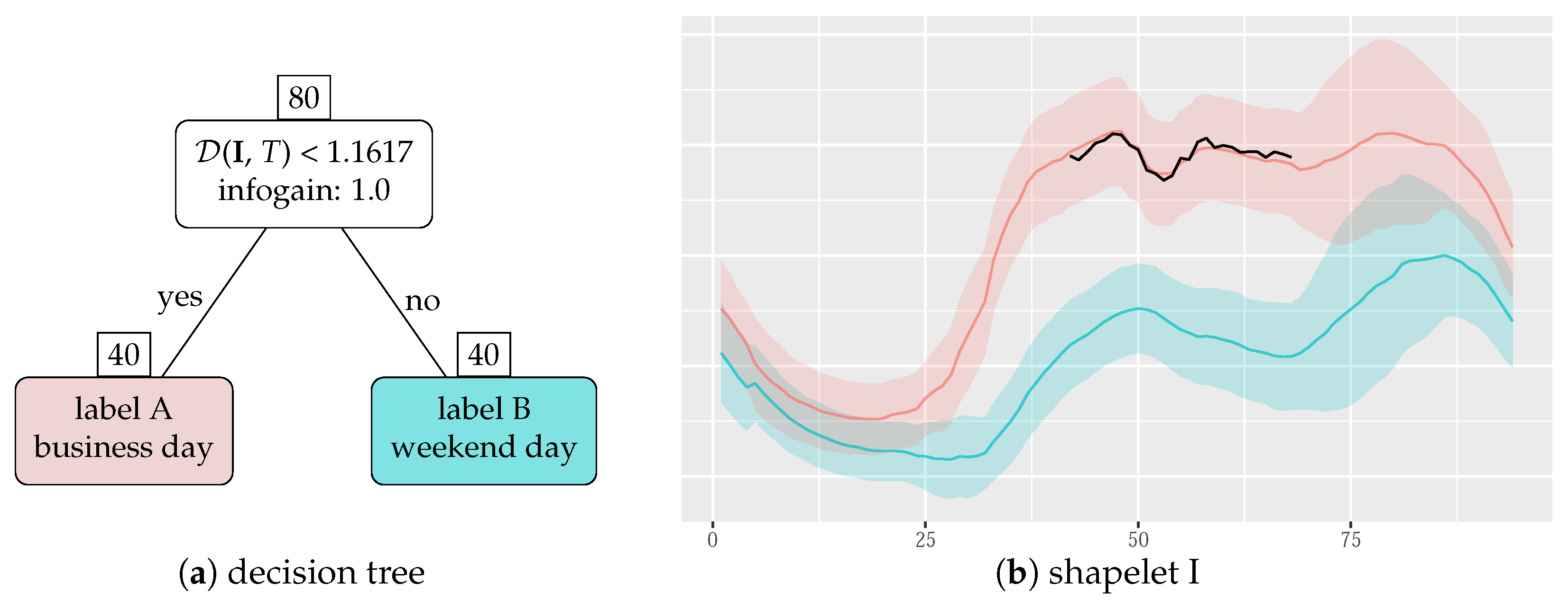
The first classification problem is related to the lower consumption that occurs on weekends. In this problem, the goal is to discover whether a 24 h time series corresponds to a weekend or a business day. As described above, the national load follows a very distinctive trend over the weekend, but even these are different over the year.
The input data are a set of time series of 96 points each (24 h with a quarter-hour resolution), extracted from the 8 year national load. Each time series has a binary classification that identifies whether it is from a business day (label A) or a weekend (label B)—
Table 1. Public holidays were separated.
Figure 3 shows us the training dataset. Note that demand throughout the daylight period is smaller on weekends, and the morning ascending occurs later and demand peaks appear at different times in the day. On the other hand, on business days, there is a demand break around lunch. We ask whether the discovery algorithm will find the best shapelet(s) to distinguish those time series.
For this scenario, the shapelet discovery algorithm is parameterized with a minimum and maximum shapelet length of 20 and 35 positions. This corresponds to shapelets between 5 and 8.75 h long, a length that we have assumed to be enough to find the shape of weekend consumption.
Figure 4 shows the decision tree obtained after the training phase. One shapelet proved to be enough to decide whether a time series
T is from a weekend or not. This results in an information gain of value 1.0 in the root node. Thus, during classification, all normalized subsequences of an arbitrary time series
T are compared with the shapelet I. If just one normalized subsequence exists whose distance to the shapelet is less than
, then the time series is classified as label A, a business day.
The resulting shapelet is 27 points long, and it is positioned in the middle of the time series, i.e., in the middle of the day. As one can see, the shapelet has grasped the demand break towards lunch—a trend which does not exist in the weekend time series. Note also that amplitude differences among the consumption time series, due to the effect of temperature or other human behavior, have not affected the accuracy of the decision tree.
Finally, the decision tree was evaluated with the testing dataset and it was found to perform with an accuracy of 96.77%.
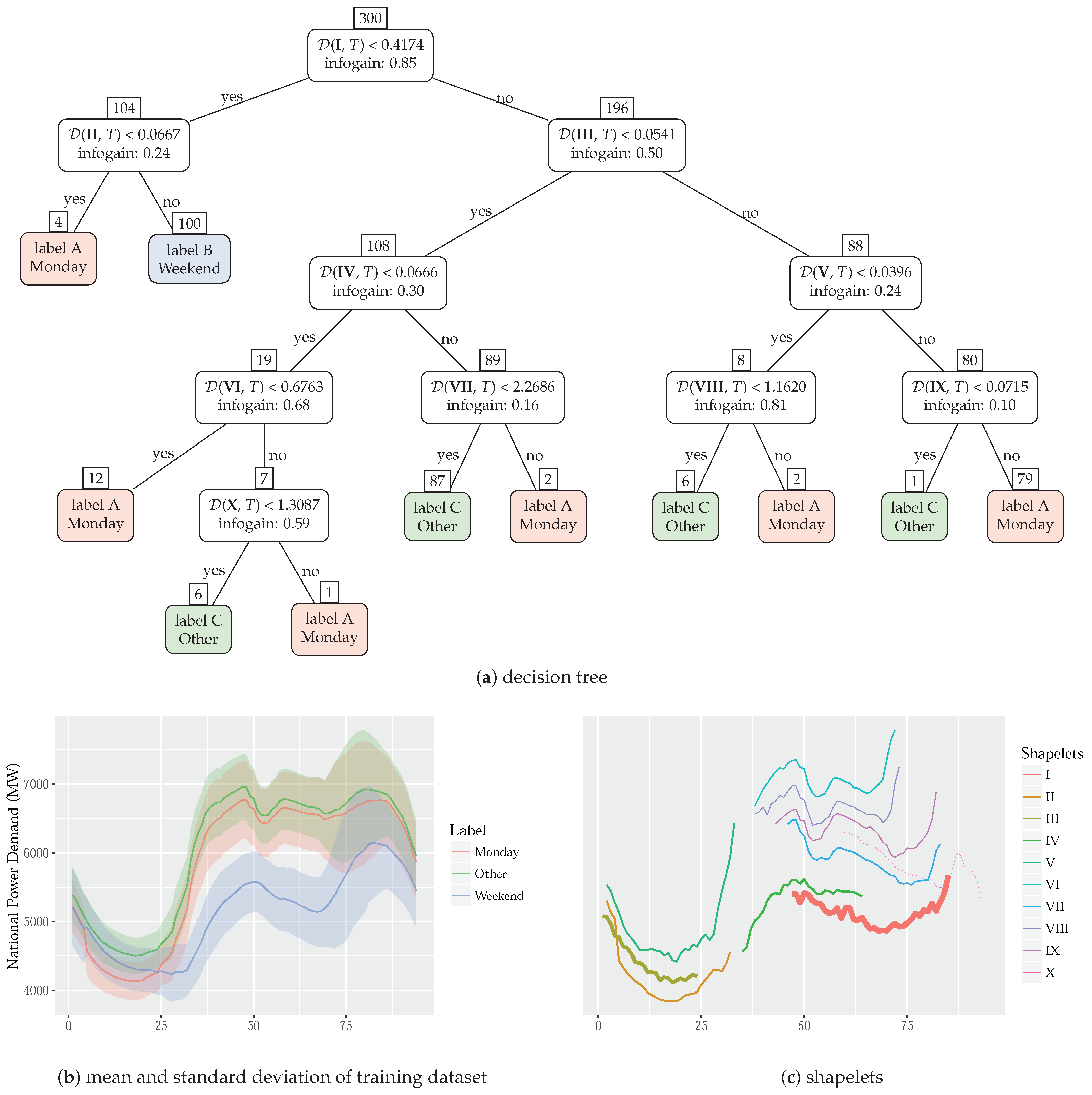
3.2. Early Monday Morning
The aim of the second classification problem is to determine whether the following result can be found using the shapelets technique. There are several publications about short-term energy forecasting that use the day of the week as an explanatory variable following this idea: Mondays are different from the rest of the business days. They detach Monday into an individual category followed by the weekend category and the rest of the days of week as another category. The rationale behind this approach is the existence of differences between the consumption during Monday’s first hours when compared with the other days, because Monday dawn comes from the end of the weekend which presents a different curve pattern as seen in the previous section. Is the shapelet algorithm able to discern the pattern presented in the Monday load curve from other business days and weekends?
The input data are similar to the previous scenario—time series of national demand and 24 hours long—but, this time, the target variable has three labels: Monday (label A), weekend (label B), and other business days (label C)—
Table 2. Public holidays were separated from the dataset.
From the training dataset—
Figure 5b—the weekend consumption pattern is distinguishable from the other days, as we saw in the previous section. However, the Monday pattern is very similar, except during the early morning. Monday’s mean demand follows a different pattern when compared with the other business days: the very first hour follows the same pattern, but the time series dives further until the first daylight hours.
The resulting non-pruned decision tree—
Figure 5a—has two important nodes that roughly split the training dataset into the three labels: the ones that use shapelets I and III. Actually, these are the nodes with the highest information gain multiplied by the number of time series to split (the number that appears above the node). In
Figure 5c, the weight of the shapelet’s line reflects its importance.
Therefore, shapelet I splits the weekend time series from the dataset (the left most branch of the decision tree). Shapelets III and V, which occur in the early morning, capture a pattern that favors class C (the opposite side of the most right branch of the decision tree). Meanwhile, the shapelet II, which also occurs in the early morning, makes a final split between the weekend time series and the Monday time series.
The non-pruned decision tree uses other similar shapelets (from VI to X), but they are not easily interpretable. However, even if those shapelets were ignored, i.e., the decision tree was pruned, the model would get right 278 times of 300 items (94%) from the training dataset.
Finally, the testing dataset was used to assess the accuracy of this decision tree. Despite its unpruned nodes and potential overfitting, the decision tree has a high accuracy of 88.74%. Evidently, there is a rationale to split Monday from the rest of business days when forecasting energy time series: the Monday demand is different from the other days and the shapelets discovery algorithm was able to find the pattern.
Furthermore, there are publications that break the business day, not into two categories but into three categories: (i) Monday, (ii) Friday, and (iii) Tuesday, Wednesday, and Thursday. We have tested this scenario, but the algorithm was not able to find a good shapelet that could accurately split time series. Indeed, the Friday time series shape is similar to Tuesday’s, Wednesday’s, and Thursday’s. In that scenario, the same method resulted in a low accuracy of 58%.
3.3. Load Dynamics in Substations
Power substations have the function of transforming energy from very high voltage (VHV) to high voltage (HV), or from high voltage to medium voltage (MV) and each usually feeds thousands of clients. As a redundant system, the power grid can manage the shutdown of a particular substation, whether due to scheduled maintenance or failure. In this situation, the load of a substation is shifted to another and thus holds out the energy flow without any significant outage. Obviously, the load time series reflects these maneuvers. While one substation reflects a very high load peak, the observations of the other reveal a stationary no-load state, see
Figure 2.
Rebuilding the historical state of this dynamic grid at a particular moment in the past can be a large computational problem due to the enormous amount of assets that change states. However, this information is important to energy forecasting tasks because of the high impact on loads due to load shifts.
In this third classification problem, we have the goal of classifying whether a substation is in one of four states looking only for the load series. Input data are a set of time series extracted from three years of historical data through a 96-point sliding window (24 h). Each time series has a label that identifies the state of the substation at the 96th point—
Table 3.
Figure 6 shows the decision tree obtained after the training phase using the first dataset. Shapelets II and IV discovered the load shifts that occurred when the grid system maneuvers the substation.
The decision tree used on the testing dataset was the non-pruned. In conclusion, the decision tree calculated with the first dataset has a high accuracy of 90%, and 83% for the decision tree using the second dataset. Furthermore, we have made experiments using sliding windows of 9 points long, SAX preprocessing of time series, fixing a state switch three points before the end of the series, or modifying the minimum and maximum lengths of candidate shapelets. However, the accuracy of the decision trees was lower, between 48% and 77%.
3.4. Type of Power Consumption
The curve of power consumption over a day depends on the purpose for which the energy is consumed. In this fourth classification problem, our objective is to classify whether power consumption serves one of these five purposes: (a) household, (b) industry, (c) services, (d) utilities, and (e) transportation. The demand curves are collected by meters of secondary substations owned by a distribution company or a high-demand client. Is the shapelets algorithm able to build a classifier capable of identifying the type of energy consumption from just the daily load curves?
The consumption data therefore refers to several sets of households or individual high-demand clients, for example: hospitals, retails, banks, post offices, government services, train and subway systems, waste water treatment plants, water pumping, gas utilities, and glass, furniture, rubber, plastics, porcelain, textiles, coating, and other types of industry.
Table 4 shows us the number of meters available by class and the number of time series extracted from them. Note that the training data were obtained from meters other than the ones used for testing. Therefore, the problem is challenging and difficult to classify, but this may be due to the low number of meters available. Additionally, the selected days were randomly chosen with the proviso that they were business days.
The resulting decision tree—
Figure 7—is fairly simple. Four shapelets are almost enough to classify the training dataset using five labels.
The shapelet I splits the dataset into two groups: one for household and transportation consumption, and the other for services, utilities, and industry. As can be seen in
Figure 8, this shapelet captures a peak in the evening as a pattern that favors “household” and “transportation” classes. Furthermore, the shapelet II splits these two labels—
Figure 9a. Since rush hour occurs twice a day, just before and after traditional work hours, it is natural that electric transportation consumes more energy during peak commuting hours.
On the other hand, shapelet III separates “industry” from the “services” demand series. In addition to the rise in the demand of both areas during the morning, and the decrease in the afternoon/evening, there is a break around lunch, which occurs only for industrial demand. Note that the descent phase of the demand for “services” extends into the evening.
Finally, the energy demand by industry and utilities presents different patterns. Utilities demand has a smoother fall in demand during the night compared to industry, and it does not get a break in demand towards lunch.
In conclusion, shapelets were able to identify the main patterns for each type of consumption, and they are quite interpretable from a domain knowledge point of view. However, the decision tree was evaluated against the training dataset and achieves only 60% accuracy. The low number of meters available may have biased the performance of shapelets in this scenario.
4. Discussion and Conclusions
In this study, the shapelet technique was applied to power load time series collected from three different hierarchical levels of the grid (national, primary power substations, and secondary power substations). Four use cases were defined considering the potential application of shapelets to answer a specific goal. This study is the first to analyze the impact of this technique in more than one use case in the energy domain, following the same methodology and at more than one grid level, while others focus on a single aspect and at a specific grid level. That was made possible by the access to real private data collected in the Portuguese smart grid and the real analytics challenges that were posed, establishing the hypothesis that power load curves alone might have inherent information capable of solving the challenges.
Shapelets have been shown to be useful for the study of pattern extraction and knowledge to understand human activities as energy consumers. This reinforces the importance of data-driven services in the energy sector that can monetize (extract additional value from) data collected within smart grids. The inability to recognize the value of the data in addition to the siloed application in which the data are collected was one of the barriers identified by the reviewers, as outlined in
Section 1. Electrification (heating and mobility as examples) and integration of more variable renewable energy (VRE), towards the ambition of 100% renewable electricity, also depend on knowing the purpose of energy consumption and whether there is flexibility on the demand side and capacity of the grid to support those two goals. The fourth use case demonstrates the possibility to classify the purpose of energy consumption and which repeatable patterns the load follows beyond the general patterns highlighted in many studies at the system level. The use case in this paper is more meticulous in the study of consumption at the primary and secondary substation level.
In particular, shapelets have shown adequate accuracy in all four use cases:
Weekends—A shapelet was enough to distinguish the daily load time series of weekends from the business days with an accuracy of 97% (
Section 3.1). The interpretable shapelet is placed in the middle of the day, and grasps the demand break during lunch, a trend that exists on business days but not on weekends.
Early Monday Morning—The resulting decision tree has a high accuracy of 89% (
Section 3.2) capable of classifying the daily load time series as weekends, Mondays, and other working days. The two most important shapelets are: (i) a similar shapelet as the previous case with the same goal, the weekend group time series, and (ii) a shapelet that occurs in the early morning on Monday morning, with lower demand—a deeper valley in the curve—when compared with other business day time series. Compared with [
16], we used data from the system level (instead of 33 buildings at the low-voltage level) with the same number of quarter-hourly training time series (namely 300 compared to 272) and a higher number of testing time series (namely, 2566 compared to 636). Although they have slightly different goals, both studies reach the same degree of accuracy (89%).
Load Dynamics in Substations—The resulting decision tree has a high accuracy between 83% and 90% for the two testing datasets (
Section 3.3), capable of identifying the substation load state, due to scheduled maintenance, failures or maneuvers, even that the load curve presents a high amplitude change by a recent maneuver.
Type of Power Consumption—The resulting decision tree has an accuracy of 60% (
Section 3.4), capable of classifying daily consumption according to the type of consumption without any other data beyond the own load curve. The amount of data available for testing may have biased the performance of shapelets in this use case. Once again, the shapelets are interpretable and reinforce the tacit and empirical knowledge practitioners might have about the consumption patterns present in different types of consumption. Compared with [
17], we used data from 28 substations (instead of 10), with load curves detailed by 96 datapoints—quarter-hourly (instead of 24 datapoints—hourly) to classify them into one of the five classes (instead of two classes). Our accuracy results reflect the classification ability of the features extracted only by shapelets, while the other study combines the shapelet features with other features to build the classifier, preventing one from pondering shapelets alone).
Thus, this study extends the literature on shapelets applied to the energy domain. At the same time, the study has some limitations, including relying solely on the shapelet technique. However, such a decision was made because of the desire to study the potential of this technique and to reinforce that the power load time series has value beyond the primary functions for which those data are collected. The second limitation is that one relies solely on a database of Portugal power load time series. This is due to the lack of real public data collected within smart grids.
Moreover, the resulting shapelets, and the decision trees that utilize shapelets while node splitting, are interpretable. Interpretability is one of the crucial characteristics in the context of electricity companies in a high-regulated business in Europe, which seeks to regulate AI across several applications, particularly models that act on or support decisions over critical infrastructure. Interpretability eases the application of data-driven services once it must be approved by managers, understandable by grid operators, and defensible before the regulator. Additionally, the interpretability of shapelets increases the knowledge of domain practitioners and, cyclically, the fact that their domain knowledge is “recognized” by the model reinforces its acceptance and adoption. Shapelets fall into the category of techniques that deliver interpretable results.
We would like to reinforce the imperative to grid operators to boost their progress toward being more data-centric and provide load curves in higher detail. This promotes research and development on innovative technologies, and accelerates the adoption of new impactful energy models, such as the integration of more VRE, development of generation and demand side flexibility, integration of more decentralized energy resources (DER), electric vehicle charging and other electric vehicle models like vehicle-to-grid (V2G) and vehicle-to-anything (V2X), microgrids, energy communities, and peer-to-peer energy (P2P energy). There are questions as to how these various energy models work together toward the energy transition and how they would be integrated into an existing grid that wants to be resilient and sustainable, both economically and environmentally.


