A Novel Approach to Predict Transformer Temperature Rise under Harmonic Load Current Conditions

Abstract

In South Africa, distribution transformers (DTs) facilitating solar photovoltaic applications represent the highest percentage of total ownership cost investment for independent power producers (IPPs). One of the most indispensable variables that regulate DTs’ operational life span is the hotspot temperature. The prevailing analytical approaches designated to guesstimate the transformer thermal necessities were fathered in accordance with the conservative foundation that an electrical transformer is prone to uniform mean daily and monthly peak loads. In order to appropriately puzzle out the transformer thermal necessities, the formation of a more detailed thermal model that operates with real-time contorted cyclic loading, ambient air temperature, and the intrinsic characteristics of the transformer in-service losses is required. In the current work, various regression models are proposed for the modification of the top-oil formula and the hotspot temperature formula in the IEEE loading guide standard to replicate the real harmonic load currents (HLCs) and the fluctuating ambient air temperature (AT) on an hourly and daily basis. The proposed thermal model is examined in various transformers case studies, in which the computed outcomes produce an error margin of no more than 3% throughout all test cases when compared to the measured data.

1. Introduction

An adaptable and thorough thermal model is a salient facet of transformer thermal necessities throughout the design phase considering that it governs the thermal ageing of the insulating materials. Such a model is vastly reliant on the produced hotspot temperature in the winding conductors of an electromagnetic field in the area nearby the uppermost winding section. The approximation and improvement of the hotspot and top-oil temperatures are ordinarily originated and governed by differential equations. In large part, thermal models attain the explanation of the set of differential equations and approximation of circuit constraints by employing Euler’s method and least square error estimation.

The authors of [1] explained a model of computing the top-oil and hottest-spot temperatures by means of statistical methods. The model enmeshes Euler’s method in elucidating the top-oil and hotspot temperature differential equations. The authors correspondingly adopted a power transformer from the IEEE guide as a pilot study to corroborate their model. In a bid to augment the thermal models, the authors of [2] presented a method to solve the governing differential equations using numerical integration. In this method, the solution of a related differential equation array is solved by utilizing the rectangular rule. In contrast to the top-oil thermal model estimated by Euler’s technique, the rectangular rule outcomes conceded furtherance in contradiction to the site measurements.

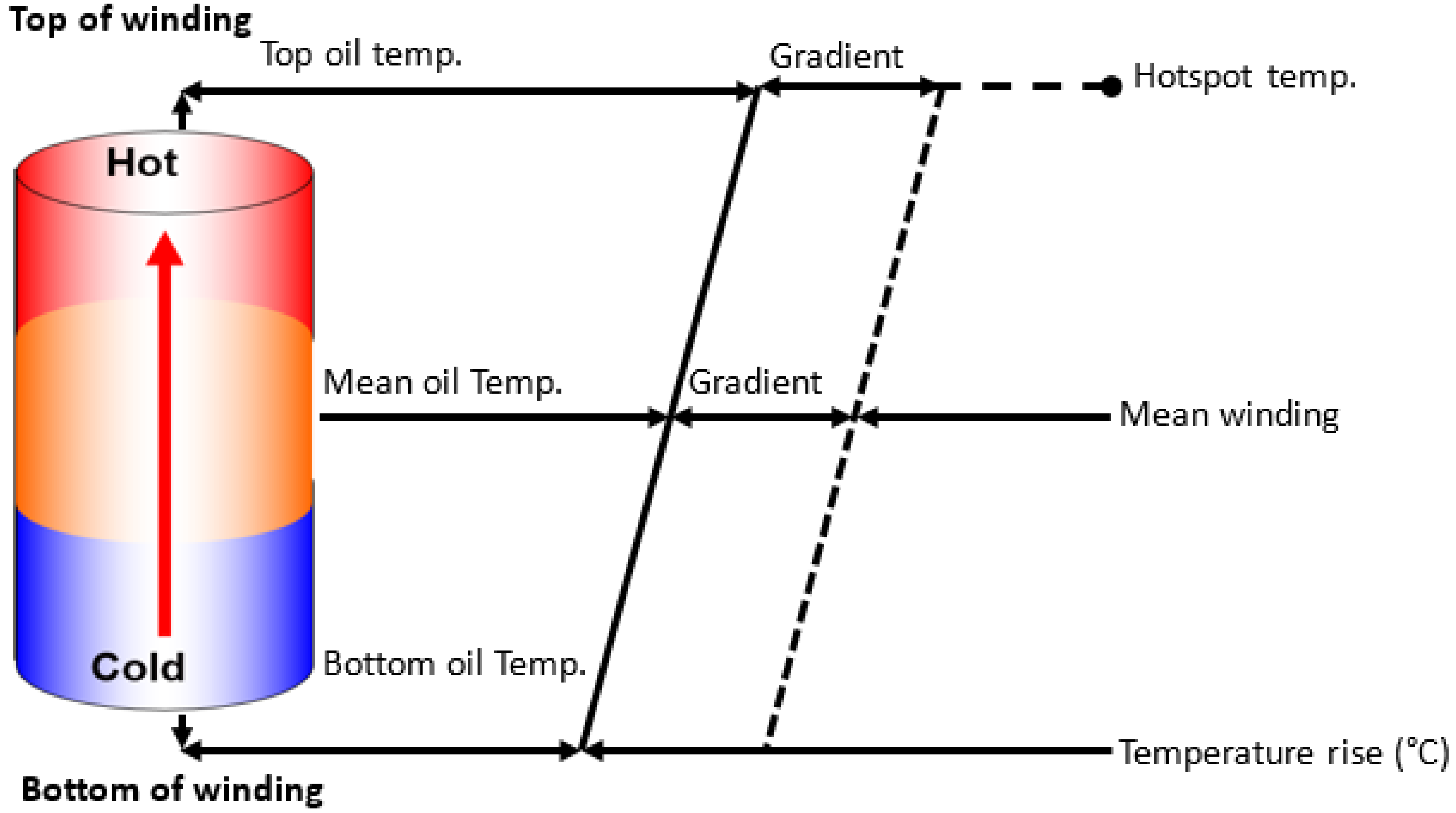
A streamlined temperature dissemination model of an oil-immersed transformer is demonstrated in Figure 1. The model elucidates the tendency of the top-oil temperature to increase in a linear fashion along with the winding distance from the bottom to the top. There is a steady temperature difference between the windings and oil cooling ducts in this linear rise in temperature. Moreover, the hotspot temperature rise surpasses the mean winding temperature (MWT), attributable to supplementary stray losses, and the proportionate hotspot factor is then accentuated by the discrepancy in the rises in the hot spot and top-oil temperatures.

Such a model is essential in this work as the real transformer thermal necessities are evaluated to set the foundation for surveying the veracity of the model and the conceptualization of the hotspot factors. Comprehensive presumptions formed in developing thermal models are discussed in the subsections below.

In [3], the IEC loading guide introduced a technique of modelling the dynamics of the top-oil and hotspot temperatures by deducing first-order differential equations. The model reflects the variations in the loading cycle as staircase functions and neglects the intermittent ambient temperature (AT). The equilibrium state of the top-oil (TOT) and hotspot temperatures (HST) are considered by means of nonlinear functions encompassing the load factor and cooling mode constraints as responding variables. Moreover, the IEC standard robustly evaluates the top-oil and hotspot temperature transient responses founded on exponential functions. The staircase function model input problem is streamlined by transforming the nonlinear and exponential function into difference equations and applying Euler’s method of approximation.

In an endeavour to develop polished thermal models, the standard [4] reformed the top-oil and hotspot temperature models presented in [3] by utilizing numerical and empirical approaches. A time constant was instituted into the top-oil temperature model to reflect the stagnant oil capacity at the bottom of the transformer steel tank. This model also incorporates the oil natural–air natural (ONAN) and oil natural–air forced (ONAF) cooling modes by employing an empirical constant denoted as K₁₁. An enhanced methodology for computing the hotspot temperature gradient is also presented in [3]. The response overshoots of the gradient are characterized by an overshoot transfer function to replicate the effect of the stagnant oil quantity in the thermal transmission of the oil movement in the cooling ducts and winding conductors. The transient transfer function is solved by the second order system of one-degree equations, with the application of the first order differential equations to transform the equations and connect them to the definitive solution of the hotspot temperature.

In [5], a method is presented to determine the thermal resistance and HST by means of a thermal circuit model. The model was established on the thermal features of the TOT of the transformer steel tank. Conversely, the foremost drawback is that the streamlined model was originated exclusively by bearing in mind other parameters playing a part in the transformer temperature rise. In [6], the authors endeavoured to advance this model by modifying the top-oil temperature recommended in [5] by employing a forecasting approach to estimate the hotspot temperature. However, the enhanced model suffers from the annexation of a considerable number of non-linear parameters exclusive of the context of a definite physical understanding. In [7], the authors formulated a thermal model for computing the temperature rise by means of the bottom-oil temperature of the transformer steel tank. The biggest problem with this model is that it fails to contemplate the environmental volatiles and the operating settings of the transformer, which can possibly lead to larger inaccuracies in the results. In [8], Zhu et al. advanced this model by contemplating the environmental volatiles, incorporating the AT and electromagnetic radiation. In [9], Gang et al. delineated a vigorous thermal model by applying the thermal circuit model methodology suggested by Swift in [5]. The model regards the Eddy losses in the winding conductors, the deviation in the oil viscidness, and the thermal resistance. By way of comparison to the temperature rise test measurements, the model produces an error margin of 3.2 K. Thermal models established by integrating the IEC thermal models with experiential data have also been reported in the publications [10,11] respectively. Based on practical knowledge, this approach is nevertheless appropriate for manufacturing specific design methodologies.

In [12], the IEEE standard reported an investigative technique to evaluate the winding hotspot temperature, discussed as the Clause 7 method. The method considers the summation of the AT, the top-oil temperature rises over the AT, and the winding hotspot over the top-oil temperature rise. In the technique, the temperature of the oil flowing out of the winding cooling ducts is presumed to be equivalent to that of the oil at the top of the steel tank. The rate of change in the top-oil temperature up to the state of equilibrium is illustrated by an exponential function encompassing a time constant that changes with the loading cycle and must be repetitiously adjusted in the computation. The biggest issue with the Clause 7 method is that it disregards thermal factors involving the change in winding resistance as a result of the hotspot temperature and AT, which is a critical factor in areas of elevated solar irradiation where solar power plants are commonly adopted. This method largely undervalues the hotspot temperature value on account of the deficiency of these thermal factors.

In [12], an alternative technique is presented to evaluate the winding hotspot temperature, stated as the Annex G method. In this method, the oil cooling duct temperature is presumed to be less than the top-oil temperature for overloading states, and the winding hotspot-over-oil temperature rise at the hottest spot region is equivalent to the top-oil temperature rise. The chief constraint of this method is that it necessitates measured values of the top- and bottom-oil temperatures, which are not always obtainable by the electrical designer in the design phase, to approximate the hotspot temperature. In the conceptualization of the regulating equations, the variations in conductor resistance and oil viscidness as a result of the temperature, rate of change in the AT, cooling mode method, and in-service no-load ($P_{NL}$) and load losses ($P_{LL}$) at varying loading profiles are contemplated. Furthermore, the Annex G method draws attention to attaining the winding hotspot temperatures by repetitiously introducing the preceding temperatures to obtain the temperature values at the subsequent instant time value. In each case, the conductor resistance, fluid viscidness, and in-service losses are recomputed for the load state.

Several scholars have also studied the top-oil and hotspot temperature models. Ishak and Wang [13] introduced a comparative examination of the HST models furnished in [12], in particular, the Clause 7 and Annex G methods. This investigation examined distinctive cooling methods and calculated the HST for numerous transformers susceptible to an incessant loading state and AT characterizations. Ishak and Wang mapped out that the Annex G method provides higher values of HST, and in the appraisal of the temperature rise test (TRT) measurements, the produced outcomes coincide. The intricacy of the Clause 7 method is instigated by the necessity to postulate the measured top- and bottom-oil temperatures, which are largely not furnished by the manufacturer for commercial use during the FATs.

In [14], a simplified model for calculating the HST with the aid of the exponential repetitious method is presented. The model is founded on the hotspot-to-ambient slope and considers the aftereffect of oil viscidness and the variance in $P_{LL}$ along with the temperature rise. The authors discovered that the model endorses the Annex G method and the temperature rise test data. Nevertheless, the shortcoming of the model is a higher initial temperature rise and the achievement of a plodding error margin as the load increases, which trivialize the impact of the oil viscidness.

Gouda et al. [15] educed a dynamic thermal model to determine the TOT and HST respectively. The model considers the distorted load currents up to the 25th harmonic order to express the supplementary in-service losses dissipating heat into the transformer active components. The TOT model was appraised on the basis of an equivalent resistance–capacitance circuit by merging the capacitances as a distinct lumped capacitance branch, while the thermal resistance component is portrayed by non-linear differential equations. In the HST model, the insulating material of thermal resistance and the oil flowing in the layers is accentuated by non-linear differential equations acquired from a thermal lumped circuit. The model introduced in this publication was authenticated alongside the IEEE model and the test results. At the individual loading cycle, the outcomes revealed a reasonable agreement. This work was utterly foundational in deducing dynamic thermal models for transformers operated in settings with high harmonic distortions.

In [2,16], a study was published that approximated the temperature rise in a 25 kVA-rated transformer employing measured data. Optical fibre sensors are optimally mounted inside the unit to attain practical data. The study contemplated an ONAN cooling method. The harmonics of the third and fifth orders investigated in this work were treated by employing a programmable voltage source. A striking upsurge of 18.4% and 46.3% in the winding mean oil temperature (MOT) slope was witnessed when the respective order of harmonics was inoculated into the transformer. Furthermore, the HSTs were augmented by approximately 8.2% and 11.8%, respectively. Under HLCs, the thermal time constant was discovered to drop slightly. These authors subsequently suggested that the thermal transient rating must be abridged when it experiences a brief period of overloading.

2. Assessment of Transformer Temperature Rise

The loading ability of transformers at the site is chiefly narrowed by the temperature in the winding conductors. In the course of the factory acceptance tests (FATs) at the manufacturer’s properties, the TRT is one of the tests carried out to confirm that during full loading conditions, as signified on the transformer nameplate drawing, the operational temperature will be as guaranteed. The MWT should not exceed the allowable temperature maxima described by the purchaser’s technical specifications and the industry recommended standards. Notwithstanding, the MWT is non-uniform, and the definite restraining parameter is the winding hotspot factor. This hotspot area is situated in the neighbouring end of the winding top attributable to the deformed axial and radial fields in the area and is not accessible for straight measurement by means of conventional methods.

The temperature introduced to the Kraft paper insulating material is a chief constituent in the ageing of a transformer. A steady rise in temperature throughout the transformer’s operational lifecycle gives rise to the decomposition of the Kraft paper insulating material. The depolymerization of the Kraft paper chains condenses the chain extent and tensile strength, which stimulates the brittleness of the transformer Kraft paper insulating material. Consequently, the Kraft paper material will capitulate to continuing electromagnetic forces and even consistent pulsations, which are integral to the transformer’s operational lifespan. This phenomenon marks the end of the cellulose insulation lifecycle and bearing in mind that it is immutable, it also marks the end of the transformer’s operational lifespan.

This process is colloquially known by power utilities and transformer manufacturers and persistent attempts have been initiated to stabilize the winding hotspot temperature (WHT) with close monitoring to subsidize low AT, extend the transformer operational lifespan while endowing the possibility of overloading capabilities and make the most of commercial opportunities. The durability tests of cellulose paper versus the WHT are illustrated in Figure 2 [3]. It should be noted that the recent evolution of thermally upgraded cellulose insulation has augmented the strength of cellulose insulation with a WHT of roughly 110 °C with respect to WHTs of 95 °C and 98 °C, as stated by the loading guides.

Furthermore, oil-immersed transformers are easily affected by growing moisture in the cellulose paper insulation when operating at high thermal states. It has been illustrated that the remnant moisture trapped in cellulose paper insulation can activate bubbling properties and the expulsion of air bubbles into the transformer oil.

The latter has been known to initiate the stray gassing of the transformer oil and supplementary decomposition of the cellulose paper insulation. This corroborates the logic for power utilities to thoroughly monitor the WHT with the most effective resources at their disposal.

In the last several decades, the IEC [3] and IEEE [4,5] standard guides have fashioned the foundation of the applauded methodologies in the transformer industry when calculating the WHT from data that can be simply measured and values of the factors attained from the TRT measurements. The rudimentary calculation methodology is reliant on the TOT taken at the top of the steel tank and the thermal slope, which is the disparity between the mean oil temperature (MOT) of the steel tank and the main windings. This value is furnished by the manufacturer as a result of oil flow modelling and the dissemination of the in-service losses in distinctive winding conductors. Therefore, the WHT appraised for a particular load can be defined according to Equation (1) [17,18,19,20].

$${\theta }_H={\theta }_{TO}+{\theta }_G\times {\left(\frac{I_L}{I_R}\right)}^{2m}$$

(1)

where

${\theta }_H—$winding hotspot temperature;

${\theta }_{TO}—$top-oil temperature;

${\theta }_G—$thermal gradient;

$I_L—$transformer load current;

$I_R—$rated transformer current;

$m—$winding cooling method exponent.

The exponential function of Equation (1) is incorporated to take into consideration the thermal inertia of the winding conductors in the event of an instantaneous rise in the transformer loading profile. This formula has been employed for many years; however, an increased application of transformer overload capability has proven this formula to be inadequate.

2.1. Transformer Thermal Model—IEC

The widely adopted thermal model in the transformer engineering industry is delineated in the IEC standards [3,4,5]. A basic illustration of the temperature dissemination along the transformer winding height is shown in Figure 3. This illustration is centred on the presuppositions enumerated as follows:

• The temperature of the oil circling along the walls of the windings rises from the bottom to the top in a linear fashion.
• The MWT circling along the walls of the windings spreads from the bottom to the top in a linear fashion, with a firm temperature differentiation $g$.
• The rise in the WHT at the top region of the winding is more than the MWT rise. To envision nonlinearity, for instance, there is an increase in the stray load losses at the top region of the windings and the top cover of the steel tank, and the distinction between the WHT and the TOT is acknowledged as $H_g$.

The HST is well thought out to encompass the summation of the thermal components as defined according to Equation (2). The AT is presumed to be unwavering. In secluded and high solar radiation areas where solar power plants would be predominantly located, an AT that increases with the HLC must be contemplated.

$${\theta }_{HS}={\theta }_A+\Delta {\theta }_{TO}+\Delta {\theta }_G$$

(2)

where

${\theta }_{HS}—$winding hotpot temperature;

${\theta }_A—$ambient temperature on-site;

$\Delta {\theta }_{TO}—$top-oil rise over the ambient temperature;

$\Delta {\theta }_G—$thermal gradient.

It follows that the rise in the TOT over ambient temperatures can be defined according to Equation (3).

$$\Delta {\theta }_{TO}=\Delta {\theta }_{T{O}_R}{\left(\frac{1+R\times K^2}{1+R}\right)}^n$$

(3)

where

$\Delta {\theta }_{TO\_R}—$TOT rise over AT at normal conditions;

$R—$ratio of $P_{LL}$ to $P_{NL}$ at normal conditions;

$K—$loading factor;

$n—$winding cooling scheme exponent.

The rise in WHT can be defined according to Equation (4).

$$\Delta {\theta }_H=H\times g\times K^{2m}$$

(4)

where

$\Delta {\theta }_H—$rise in the hotspot temperature;

$H—$hottest spot factor;

$g—$ratio of MWT to top-oil;

$m—$exponent of the transformer cooling system.

The indorsed exponents of the transformer cooling systems pronounce the nonlinearity point in the rise in stray losses at the top region of the winding and top cover of the steel tank. The winding cooling method exponents supported by the IEEE and IEC are classified as follows in

Table 1. Exponents of the transformer cooling systems.

Cooling Systems	IEEE		IEC
	m	n	m	n
ONAN	0.8	0.8	0.8	0.9
ONAF	0.8	0.9	0.8	0.9
Non-directed OFAF or OFWF	0.8	0.9	0.8	1.0
Directed ODAF or ODWF	1.0	1.0	1.0	1.0

$\mathrm{ONAN}—$oil natural–air natural, $\mathrm{ONAF}—$oil natural–air forced, $\mathrm{OFAF}/\mathrm{OFWF}—$oil forced–air forced/oil forced–water forced, $\mathrm{ODAF}/\mathrm{ODWF}—$oil directed–air forced/oil directed–water forced.

.

2.2. Evaluation of the Hotspot Factor

In the variety of tests conducted at the testing bay, the MWT attained by the TRT capitulated to emulate the amplification in losses resulting from the Eddy currents condensed in the areas towards the top and bottom winding ends. These losses are compensated for by the hotspot factor (HSF) designed to meet the needs of computing the absolute WHT. In the experience-based data released by the CIGRE Working Group to corroborate the HSF indorsed by the IEC standard [3,4,5], the outcomes suggest that the values of the HSF that fall into the region between 1 and 1.5 correspond to the transformer design particulars. Apropos of small (SPTs) and medium (MPTs) power transformers, the HSF values of approximately 1.1 and 1.3 have been specified. In large power transformers (LPTs), the HSF values vary considerably, contingent on the design particulars, and the manufacturer should be provided with correct data, excluding cases where measurements have been performed.

Directly measured WHT data accentuate that the degree of variance in the HSF exists within the approximate values of 1.1 and 2.2. Moreover, the HSF is not constant and must be estimated correctly for the individual transformer design, bearing in mind that in reality, an unfeasible value will not allow the manufacturer to ascertain the loading capability of the transformer, while an unusually low value undervalues the absolute WHT.

The CIGRE research group advocates numerous formulae for calculating the HSF to vindicate the degree of variance of the HSF and project fitting value for designing a specific transformer. However, no version has been approved.

2.3. Direct Measurement of HSF

The TRT can be immaculately measured through fibre optic sensors (FOS) positioned in the transformer winding conductors in the course of the process of manufacturing, as presented in Figure 4. This methodology may not be practical for existing transformers and may be difficult to corroborate the value for new transformers.

The FOSs are responsible for recording the winding temperatures solely in the areas where the sensors are positioned. A befitting option for setting the FOSs in consonance with the windings is critical to suitably mirror the WHT. As a consequence, their veracity in measuring the WH is subject to their proficiency in predicting the regions of hotspots prior to the insertion of the FOSs. Although FOSs have some fundamental deficiencies, they are still regarded as the best methodology for appraising the WHT.

2.4. Thermal Model for Transformers Facilitating HLCs—IEEE

In transformers designed for an ONAN cooling system, the calculation of the TOT is completely analogous to the loss ratio as specified to the power of 0.8, as indicated in Equation (5), and can be evaluated for the HLC profile furnished by the purchaser at the inquiry phase.

$${\theta }_{TO}={\theta }_{TO\_R}\times {\left(\frac{P_{LL}+P_{NLL}}{P_{LL\_R}+P_{NLL}}\right)}^{0.8}$$

(5)

where

${\theta }_{TO}—$top-oil temperature under HLCs (°C);

$P_{LL}—$load loss under HLCs ($\mathrm{kW}$);

$P_{NLL}—$no-load loss under HLCs ($\mathrm{kW}$);

$P_{LL\_R}—$no-load loss at rated conditions ($\mathrm{kW}$).

Subsequently, the WHT rise over the TOT can be defined according to Equation (6).

$${\theta }_g={\theta }_{g\_R}\times {\left(\frac{I^2\left(pu\right)\times \left(1+F_{HL}+P_{EC\_R}\right)}{1+P_{EC\_R}}\right)}^{0.8}$$

(6)

where

${\theta }_g—$thermal gradient under HLCs (°C);

${\theta }_{g\_R}—$thermal gradient at rated conditions (°C);

$F_{HL}—$winding Eddy loss harmonic factor;

$P_{EC\_R}—$winding Eddy loss at rated conditions (p.u).

It follows that the WHT can be defined according to Equation (7).

$${\theta }_{TO}={\theta }_{TO}+{\theta }_{TO}$$

(7)

where

${\theta }_{HS}—$hotspot temperature under HLCs.

The temperature rise formulae reported in the IEEE C57.110-2018 standard stands in need of alteration to properly capture the particulars for transformers in service to solar power plants in the South African grid.

In recent studies [21,22,23], the authors have also reported some work based on artificial intelligence to estimate the HST.

3. Materials and Methods

The HST in the transformer winding conductors can be distinguished as the most crucial technical parameter in instituting the transformer loading withstand. It incites the thermal ageing of the Kraft paper and oil insulating systems and the conceivable possibility of stray gassing abnormalities. This has made it increasingly important for the power producers to be educated on the HST of the transformer at respective harmonic loading conditions and hourly AT. The techniques for estimating the ${\theta }_{TO}$, ${\theta }_{TO} ,$ and ${\theta }_{TO}$ for transformers, specifically in service to HLCs, are defined in the IEEE C57.110-2018 standard. These approaches do not appropriately address the rated thermal parametric procedures for estimating the aforesaid thermal factors for transformers operating in particular solar power plant conditions.

In the current work, the procedure for a standard rated thermal design of units projected to operate in the South African grid utilizing local technical particulars is well-established. The methods for evaluating the ${\theta }_{TO}$, ${\theta }_{TO},$ and ${\theta }_{TO}$ have been protracted and revised by inserting the regression models and the hourly AT with a view to contemplate the thermal, in-service losses and AT necessities for transformers operating under HLCs in the South African grid. The approaches proposed in this work are indispensable to ascertaining the loading capability of both recently designed and existing transformers. The approaches should be comprehensive and practical, as shown in Figure 5.

3.1. Transformer Thermal Modelling

A comprehensive investigation of solar power transformers operating in the South African grid was conducted with a focus on formulating a guideline for specifying the practicable in-service losses and thermal constraints is presented. The study was performed by formulating regression models to acquire several guides for three-phase, 50 Hz transformers extending from 100 kVA to 40 MVA with the highest primary voltage of 132 kV. It is emphasized that the regression models established in the magnitude of this work refer to the experiments to close the information gaps in the technical standards involving transformers, which are wholly projected to operate in solar photovoltaic applications.

3.2. Proposed Top-Oil Model

The formulae for appraising the HST need to be improved to integrate the increase in the transformer in-service losses and the comparative hotspot temperature. The loss ratio ($P_{ratio\left(new\right)}$) should echo the real HLCs that the transformer will be exposed to during operation.

The TOT equation in the IEEE C57.110-2018 standard has been revised to mirror the real HLCs that the transformer will be prone to during operation. The TOT formula illustrated in Equation (4) was improved and is defined according to Equation (8).

$${\theta }_{TO\left(new\right)}={\theta }_{TO\_R\left(new\right)}\times {\left(P_{ratio\left(new\right)}\right)}^{0.8}$$

(8)

where ${\theta }_{TO\_R\left(new\right)}$ is the proposed TOT in the steel tank at rated conditions (°C). The latter can be nominated for the novel regression models illustrated in

Table 2. Novel TOT models at rated conditions (°C).

VA Range	${\mathit{\theta }}_{\mathit{T}\mathit{O}\_\mathit{R}\left(\mathit{n}\mathit{e}\mathit{w}\right)}$	${\mathit{R}}^2$
Up to 100 kVA	$30.42+0.0131 \mathrm{kVA}+0.0108 \mathrm{HV}$	0.9069
100.1–315 kVA	$32.22+0.0077 \mathrm{kVA}+0.0119 \mathrm{HV}$	0.9920
315.1–5 MVA	$37+0.0015 \mathrm{kVA}+0.0178 \mathrm{HV}$	0.9214
10–40 MVA	$43.28+0.168 \mathrm{MVA}+0.016 \mathrm{HV}+0.0124 \mathrm{LV}$	0.9584

.

The loss ratio in Equation (8) has been modified as follows:

$$P_{ratio\left(new\right)}=\left[\frac{P_{NLL\left(new\right)}+P_{cu\_R\left(new\right)}+P_{WE{C}_R}{{\displaystyle \sum }}_{h=1}^{h=max}{h}^2{\left(\frac{I_h}{I_R}\right)}^2+P_{OS{L}_R}{{\displaystyle \sum }}_{h=1}^{h=max}{h}^{0.8}{\left(\frac{I_h}{I_R}\right)}^2+P_{NLL\left(new\right)}}{P_{LL\_R\left(new\right)}+P_{NLL\left(new\right)}}\right]$$

Accordingly, the proposed no-load losses ($P_{NLL\left(new\right)}$) may be assessed in accordance with

Table 3. Proposed regression models for $P_{NLL\left(new\right)}$.

VA Range	${\mathit{P}}_{\mathit{N}\mathit{L}\mathit{L}\left(\mathit{n}\mathit{e}\mathit{w}\right)}$	${\mathit{R}}^2$
Up to 100 kVA	$40.61+1.92 \mathrm{kVA}+1.22 \mathrm{HV}$	0.9276
100.1–315 kVA	$125.11+1.89 \mathrm{kVA}+4.57 \mathrm{HV}$	0.9087
315.1–5 MVA	$580.945+1.125 \mathrm{kVA}+11.366 \mathrm{HV}$	0.9592
10–40 MVA	$4.0926+0.2208 \mathrm{MVA}+0.0088 \mathrm{HV}+0.0017 \mathrm{LV}$	0.9528

.

The regression models for the $P_{NLL}$ produce a good correlation coefficient extending from 0.97 to 0.99. Consequently, the copper losses ($P_{cu\_R\left(new\right)}$) may be assessed in accordance with

Table 4. Proposed regression models for $P_{cu\_R\left(new\right)}$.

VA Range	${\mathit{P}}_{\mathit{c}\mathit{u}\_\mathit{R}\left(\mathit{n}\mathit{e}\mathit{w}\right)}$	${\mathit{R}}^2$
Up to 100 kVA	$272.51+10.46 \mathrm{kVA}+8.16 \mathrm{HV}$	0.9104
100.1–315 kVA	$2527.54+1.76 \mathrm{kVA}+4.16 \mathrm{HV}$	0.9077
315.1–5 MVA	$2020.3+4.85 \mathrm{kVA}+40.733 \mathrm{HV}$	0.9476
10–40 MVA	$-22.1695+5.3303 \mathrm{MVA}+0.2230 \mathrm{HV}+0.2017 \mathrm{LV}$	0.9804

.

Moreover, the winding Eddy losses $P_{EC\_R}$ that mirror the real HLCs can be defined according to Equation (9).

$$P_{EC\_R}=P_{cu\_R\left(new\right)}\times {{\displaystyle \sum }}_{h=1}^{h=max}{h}^2{\left(\frac{I_h}{I_R}\right)}^2$$

(9)

The proposed winding Eddy losses ($P_{EC\_R\left(new\right)}$) may be assessed in accordance with

Table 5. Novel regression models for the $P_{EC\_R\left(new\right)}$.

VA Range	${\mathit{P}}_{\mathit{E}\mathit{C}\_\mathit{R}\left(\mathit{n}\mathit{e}\mathit{w}\right)}$	${\mathit{R}}^2$
Up to 100 kVA	$19.2+0.74 \mathrm{kVA}+0.57 \mathrm{HV}$	0.9104
100.1–315 kVA	$162.27+0.198 \mathrm{kVA}+0.181 \mathrm{HV}$	0.9159
315.1–5 MVA	$875.72+0.23 \mathrm{kVA}+3.612 \mathrm{HV}$	0.9117
10–40 MVA	$-5.48 \mathrm{MVA}+0.5851 \mathrm{HV}+0.0117 \mathrm{HV}-0.0025 \mathrm{LV}$	0.9616

.

Additionally, the other stray losses $P_{OSL}$ that mirror the real HLCs can be defined according to Equation (10).

$$P_{OSL=}{P}_{OSL\_R\left(new\right)}\times {\displaystyle \sum }_{h=1}^{h=max}{h}^{0.8}{\left(\frac{I_h}{I_R}\right)}^2$$

(10)

The proposed other stray losses ($P_{OSL\_R\left(new\right)}$) may be evaluated by applying

Table 6. Novel regression models for $P_{OSL\_R\left(new\right)}$.

VA Range	${\mathit{P}}_{\mathit{O}\mathit{S}\mathit{L}\_\mathit{R}\left(\mathit{n}\mathit{e}\mathit{w}\right)}$	${\mathit{R}}^2$
Up to 100 kVA	$27.3+1.05 \mathrm{kVA}+0.82 \mathrm{HV}$	0.92
100.1–315 kVA	$221+0.307 \mathrm{kVA}+0.23 \mathrm{HV}$	0.93
315.1–5 MVA	$1254+0.34 \mathrm{kVA}+5.17 \mathrm{HV}$	0.91
10–40 MVA	$-7.35+0.6644 \mathrm{MVA}+0.0397 \mathrm{HV}-0.0233 \mathrm{LV}$	0.94

.

Ultimately, the total load losses ($P_{LL\left(new\right)}$) can be defined according to Equation (11).

$$P_{LL\left(new\right)=}{P}_{cu\_R\left(new\right)}+P_{WE{C}_R}{{\displaystyle \sum }}_{h=1}^{h=max}{h}^2{\left(\frac{I_h}{I_R}\right)}^2+P_{OS{L}_R}{{\displaystyle \sum }}_{h=1}^{h=max}{h}^{0.8}{\left(\frac{I_h}{I_R}\right)}^2$$

(11)

3.3. Transformer Thermal Gradient (Proposed)

The improved thermal gradient can be defined according to Equation (12).

$${\theta }_g={\theta }_{g\_R\left(new\right)}\times {\left(\frac{I^2{}_{pu}\times \left(1+HLF\times P_{EC\_R\left(pu\right)}\right)}{1+P_{EC\_R\left(pu\right)}}\right)}^{0.8}$$

(12)

The proposed thermal gradient (${\theta }_{g\_R\left(new\right)}$) may be evaluated with the data in

Table 7. Proposed regression models for ${\theta }_{g\_R\left(new\right)}$.

VA Range	${\mathit{\theta }}_{\mathit{g}\_\mathit{R}\left(\mathit{n}\mathit{e}\mathit{w}\right)}$	${\mathit{R}}^2$
Up to 100 kVA	$4+0.0017 \mathrm{kVA}+0.0014 \mathrm{HV}$	0.9069
100.1–315 kVA	$4.42+0.00011 \mathrm{kVA}+0.0016 \mathrm{HV}$	0.9891
315.1–5 MVA	$5.3+0.002 \mathrm{kVA}+0.00025 \mathrm{HV}$	0.9220
10–40 MVA	$5.5492+0.164 \mathrm{MVA}+0.011 \mathrm{HV}+0.0048 \mathrm{LV}$	0.9918

.

3.4. Transformer HST

The HST equation, as noted in the IEEE C57.110-2018 standard, has been tailored to mirror the wavering AT on an hourly rate over a 24-h period. The HST can be defined according to Equation (13).

$$\Delta {\theta }_{HS}=\Delta {\theta }_A+\Delta {\theta }_{TO}+\Delta {\theta }_g$$

(13)

The AT was integrated into the HSR equation to vigorously identify the environmental states on-site. The AT characteristics for a solar plant installed in the Northern Cape allow for the values presented in Figure 6.

In the following section, numerous case studies have been introduced for the purpose of substantiating the proposed approach.

3.5. TRT Measurements

In consideration of substantiating the practicability and reliability of the proposed thermal model, a TRT was performed. The TRT is a critical test that should be an integral part of testing for all oil-immersed transformers. In the test, the restriction of the rise in temperature in the windings and insulating oil was corroborated as warranted by the original equipment manufacturer (OEM). Thermocouple probes illustrated in Figure 7 were positioned to measure the dissemination of the temperature of the studied transformer case studies. The test was carried out in compliance with the IEC 60076-7 guidelines.

The short circuit method, as demonstrated in Figure 6, was applied to carry out the TRT by injecting a high voltage winding while the low voltage winding was still short-circuited. As exhibited, the thermocouple probes were placed near the top cover of the transformer steel tank. The electric potential injected into the high voltage winding was a summation of the $P_{NLL}$ and $P_{LL}$ adjusted to a reference temperature of 75 °C. During the TRT, hourly readings of the TOT were witnessed with the aid of the thermocouple probes. The AT at the manufacturer’s test bay was measurable by the insertion of thermometers at four locales 2 m away from the cooling surface of the unit tested. The ultimate rise in the TOT was acquired at a point where it arrived at a state of equilibrium and increased no more than 3 °C at an hourly rate.

4. Case Studies

In this section, the case studies comprising TRT data have been documented for four transformers. The approaches for appraising the Eddy current losses when a transformer is in-service to HLCs were compared employing the proposed numerical methods, the Emanuel et al. approach, and the IEEE C57.110-2018 method. Furthermore, hourly data on the HST were also demonstrated.

The case studies examined in this work were planted with fibre optic thermal sensors (FOTS) in the primary windings. The active component structures were equipped with thermocouple probes.

4.1. Case Study 1: 40 MVA 88/11 kV Distribution Transformer

The augmentation in the winding temperature was supervised on the 88 kV primary winding and the secondary 11 kV winding. The percentage impedance of this transformer was 8% as per the technical particulars. The oil dissemination in the winding conductors was piloted by oil guiding rings arranged in a zigzag model. This unit was equipped with eight FOTS—four on the 88 kV primary winding and four on the secondary 11 kV winding. The measurement of the ${\theta }_{TO\_R}$ and the ${\theta }_{g\_R\left(new\right)}$ was carried out on the ONAN cooling type, as illustrated in

Table 8. Case study 1: 40 MVA 88/11 kV distribution transformer.

$\mathbf{Temperature} (°C)$	Measured Value	Proposed Model	Error Margin
${\theta }_{g\_R\left(new\right)}$	13.21	13.1325	0.59%
${\theta }_{TO\_R}$	51.55	51.5220	0.05%

.

It can be observed that the novel model appraised the ${\theta }_{g\_R\left(new\right)}$ and ${\theta }_{TO\_R}$ parameters with practical precision; a wonderful asset that can be utilized by electrical engineers throughout the design of technical particulars for solar PV transformers in the South African grid. Moreover, transformer manufacturers can utilize the proposed regression models as guides for designing power transformers.

The HST measurements that were measurable in a 24-h cycle in the location of the Northern Cape province were documented throughout a month of high solar radiation and are in line with the outcomes calculated by the proposed winding Eddy loss HLF and the existing method reported by Emanuel et al. The comparison outcomes are demonstrated in Figure 8.

The highest computed winding HSTs by the IEEE method, novel approach, and Emmanuel et al. approaches are 139.31, 134.60 and 140.65, respectively.

It should be underlined that the winding designated for comparative examination in this case study was the hottest. Figure 7 graphically exhibits the dynamic hourly HST.

4.2. Case Study 2: 10 MVA 22/11 kV Distribution Transformer

The temperature rises in this unit were supervised on the primary and secondary windings. The unit has a star–delta (YNd1) vector group with a percentage impedance of 8% and an ONAN cooling system. The oil distribution in the windings was piloted by oil guiding rings constructed in a zigzag model. This transformer was planted with 16 FOTS—8 in the primary winding and 8 in the secondary winding, respectively. By and large, 14 thermocouple probes were placed in various active component structures at the upper band of the secondary winding.

Table 9. Case Study 2: 10 MVA 22/11 kV distribution transformer.

$\mathbf{Temperature} (°C)$	Measured Value	Proposed Model	Error Margin
${\theta }_{g\_R\left(new\right)}$	7.26	7.4846	3%
${\theta }_{TO\_R}$	45.15	45.4447	0.65%

shows a tabulation of the comparative examination of the 10 MVA 22/11 kV distribution transformer utilizing the measured and proposed regression model.

The novel approach was observed to produce an error of no more than 3% when compared to the measured values. The latter corroborate the dependability of the proposed approach. The hourly HST disparities are in line with the outcomes attained from the thermal models as demonstrated in Figure 9.

It should be emphasized that the winding designated for the comparative examination of this transformer was the hottest. Figure 9 graphically displays the vigorous hourly HST. The highest computed winding HST by the IEEE method, the novel approach, and the Emmanuel et al. approach are 125.91, 122.98, and 126.75, respectively.

4.3. Case Study 3: 5000 kVA 33/0.42 kV Distribution Transformer

The results of a comparative examination of the 5000 kVA 33/0.42 kV distribution transformer utilizing the measured and proposed regression model are exhibited in

Table 10. Case study 3: 5000 kVA 33/0.42 kV distribution transformer.

Method	Measured Value	Proposed Model	Error Margin
${\theta }_{g\_R\left(new\right)}$	6.3	6.4362	2.12%
${\theta }_{TO\_R}$	44	45.1	2.44%

. This unit was equipped with 14 FOT—8 in the 33 kV primary winding and 8 in the 0.42 kV secondary winding, respectively.

The proposed model was observed to produce an error of no more than 2.5% in comparison to the measured data. The HST variations on an hourly basis are in line with the means of the results attained using the thermal models as demonstrated in Figure 10.

The estimated winding HSTs by the IEEE guide, the novel approach, and the Emmanuel et al. technique are 132.24, 128.38, and 133.34, respectively. It should be underlined that the winding designated for comparability in this unit was the hottest. Figure 10 illustrates the vigorous hourly hotspot temperature.

5. Conclusions

As part of this work, an improved thermal model that can detect the thermal characteristics of oil-immersed distribution transformers principally operating with solar PVs in the South African grid was proposed and corroborated. Firstly, regression models for the losses, namely the $P_{NLL\left(new\right)}$, $P_{cu\_R\left(new\right)}$, $P_{cu\_R\left(new\right)},$ and $P_{OSL\_R\left(new\right)} \mathrm{were}$proposed. Moreover, the consonant ${\theta }_{TO\_R\left(new\right)}$ and ${\theta }_{g\_R\left(new\right)}$ regression models were also proposed. Thermal modelling for transformers in solar power plants must mirror the influence of HLCs that the transformer will be exposed to during operation. The $P_{ratio}$ should be such that it reflects the real HLCs that the transformer will be at risk of during operation at the site.

The TOT and HST formulae in the IEEE C57 standard were amended to echo the actual HLCs and the erratic AT on an hourly rate over 24 h. The formulated thermal model was verified in several oil-immersed transformer case studies, in which the computed outcomes produced an error of estimate of no more than 3% throughout the case studies when compared to the measured data.

The developed thermal model is an economical and effective design tool for appraising the temperature rise in transformers projected to service solar power plants in the South African grid.