An Iterative Algorithm for the Estimation of Thermal Boundary Conditions Varying in Both Time and Space

Abstract

The presented survey of the up-to-date state of knowledge indicates that despite the great number of works devoted to the issue in question, there is no simple method that allows the use of commercial programs for the identification of the transient thermal state in elements with a simple or complex shape. This paper presents an inverse method developed to estimate the convective heat transfer coefficient varying both in time and space on a vertical plate during its cooling. Despite the smaller number of measurement points and larger disturbance of measured temperatures compared to the data presented in the available literature, comparable results are obtained. The developed iterative algorithm is also applied to estimate the time- and space-dependent heat flux and the convective heat transfer coefficient in the steam boiler membrane waterwall. The analysed component has the form of the non-simply connected and complex shape domain Ω. Temperature-dependent thermophysical properties are used. Calculations are performed for the unknown heat flux or heat transfer coefficient distribution on the domain boundary based on measured temperature transients disturbed with a random error of 0.5 °C. To reduce oscillations, the number of future time steps of N_F = 20 is selected. The number of iterations in each time step ranges between 1 and 8. The estimated boundary conditions are close to the exact values. In this work, the ANSYS software using the FEM is applied.

1. Introduction

Modelling heat and fluid flows as well as thermal-, flow-, and strength-related processes plays an important role in the design and operation in engineering. The influence of the real ground temperature on a building’s heat loss is analysed in [1]. The numerical model of heating and cooling unit with a reversible heat pump based on CO₂ is presented in [2]. Its experimental validation is also reported. Paper [3] presents a novel crossflow air–to–water heat exchange, its experimental testing, and modelling. A thermal and strength analysis of the power boiler superheater is shown in [4]. The maximum operating temperature is calculated by the proposed creep equation. The transient-state distribution of thermal stresses in a steam gate valve and the proposition of optimization algorithm for heating and cooling operations is presented in [5]. The significant problem of modelling the temperature and stress distributions in newly designed and used components causes the difficulty in defining some of the boundary conditions. Modelling requires the specification of dimensions, thermophysical properties, source terms, boundary conditions or initial conditions. The more precisely the input data are determined, the better the modelling results are. In practice, it is often difficult to define the boundary conditions. Placing thermocouples on the inner surface of CFB furnace, superheater chambers, pipelines, as well as gates and valves can destroy them [6]. A direct temperature measurement on the outer surface of an atmospheric re-entry capsule is difficult due to its high value [7].

A boundary condition that is difficult to define can be considered as unknown, and additional information can be added to the analysis. An analysis defined in this way is called an inverse boundary problem. For components with simple shapes, one-dimensional temperature distribution and constant material properties’ exact methods can be used [8]. A certain inconvenience of the proposed solutions is the need to take a larger number of terms in the series describing the temperature distribution. If the number of terms is not high enough, the temperature distribution calculated at the initial time instant will differ from the real one. For multidimensional problems, finding a solution is laborious [9]; therefore, numerical methods are used. Nonlinear one-dimensional inverse problems may be solved by means of the finite difference method (FDM) [10]. The proposed method for a two-dimensional problem [11] has a global character, which means that calculations may be started only after measurements are performed, when the temperature histories from the initial to the final time instant have been recorded. For this reason, the methods cannot be used for online identification of the temperature distribution in the element. An optimization method intended for solving multidimensional inverse problems was proposed in [12]. In [13], an online inverse space marching method based on the control volume method (CVM) in cylindrical coordinates was formulated. The proposed method was applied to identify the transient-state two-dimensional temperature estimation in the steam header cross-section and to reconstruct the unknown boundary condition on its inner surface. A numerical algorithm for determination of the heat transfer coefficient distribution on a vertical plate under mixed-convection conditions was developed in [14] using a two-dimensional inverse method. Applications of a modified Levenberg-Marquardt method for identification of the conductivity and heat capacity of solids is presented in [15,16].

The presented survey of the up-to-date state of knowledge indicates that despite the great number of works devoted to the issue in question, there is no simple method that allows the use of commercial programs for the identification of the transient thermal state in elements with a simple or complex shape. The methods published so far require writing the source code with the use of FDM or CVM.

This paper presents a method developed to estimate the convective heat transfer coefficient varying both in space and time. The proposed method is used to estimate the heat transfer coefficient distribution of a vertical plate during cooling under the mixed-convection regime. The estimated values are compared to those calculated in [6]. Despite the smaller number of measurement points and larger disturbance of the measured temperatures, the obtained results are comparable to [14]. Additionally, the proposed method is easier to apply as it allows the use of commercial programs. The developed iterative algorithm is also applied to estimate the heat flux and the convective heat transfer coefficient varying over time in the steam boiler membrane waterwall. The analysed component has the form of the non-simply connected domain Ω.

2. Formulation of the Method

The transient heat conduction problem in the non-simply connected domain Ω shown in Figure 1 can be described using the following equation [17]:

$$c\left(T\right)\rho \left(T\right)\frac{\partial T}{\partial t}=-\nabla ·q$$

(1)

where q is the heat flux vector defined by Fourier’s law:

$$q=-D\nabla T$$

(2)

and

$$D=\left[\begin{array}{ccc}{k}_x\left(T\right)& 0& 0\\ 0& k_y\left(T\right)& 0\\ 0& 0& k_z\left(T\right)\end{array}\right]$$

(3)

If the material is isotropic, then $k_x\left(T\right)=k_y\left(T\right)=k_z\left(T\right)=k\left(T\right)$. All material properties (c—specific heat, k—thermal conductivity, and ρ—density) are usually known functions of temperature. Fourier’s law applies to all engineering applications for which the infinite speed of a heat propagation can be assumed. Transient heat conduction problems are initial–boundary problems for which appropriate initial and boundary conditions should be defined [17]. The initial condition specifies the temperature value of the non-simply connected domain Ω at its first moment t₀ = 0 s:

$${T\left(x,y,z,t\right)|}_{t_0=0}=T_0\left(x,y,z\right)$$

(4)

One of the first-, second-, or third-kind boundary conditions should be defined on boundary $\Gamma ={\Gamma }_{in}\cup {\Gamma }_{out}$

$${T|}_{\Gamma }=T_b$$

(5)

$${\left(D\nabla T·n\right)|}_{\Gamma }=q_B$$

(6)

$${\left(D\nabla T·n\right)|}_{\Gamma }=h\left(T_m-{T|}_{\Gamma }\right)$$

(7)

where n—unit normal vector to boundary, T_b—temperature on the domain boundary, $q_B$–heat flux on the domain boundary, h—heat transfer coefficient on the domain boundary Γ, and T_m—temperature of the medium. A phenomenon characterized by Equations (1)–(7) in which all dimensions, properties, the initial condition, and the boundary conditions over the entire boundary $\Gamma ={\Gamma }_{in}\cup {\Gamma }_{out}$ are specified is known as a direct transient heat conduction problem. If part of boundary conditions (5)–(7) is unknown, the problem is ill-posed, and additional internal temperature measurements are required

$$f_i\left(t\right)=T\left(r_i\right) i=1, \dots , N_T$$

(8)

The unknown first-, second-, or third-kind boundary condition is divided into N_u intervals. It can be approximated as a staircase or a polynomial function on the domain edge (Figure 2).

The aim is to choose time-varying $u\left(u_1\left(t\right),u_2\left(t\right),\dots ,u_{N_u}\left(t\right)\right)$ such that the calculated temperatures are close to the temperature values obtained from the experimental measurements. This can be expressed as:

$$T_i\left(u,r_i,t\right)-f_i\left(t\right)\cong 0, i=1,\dots ,N_T$$

(9)

The number of measurement points N_T cannot be smaller than the number of unknown boundary condition intervals N_u. Ill-posed problems are tough to solve. They are sensitive to errors in input data. Many algorithms can be adopted to stabilise the solution. Future time steps are applied in this paper. To stabilise the solution, vector u_L is held constant in N_F future time steps [18], as can be seen in Figure 3.

$$u_L=u_{L+1}=\dots =u_{L+N_F-1}$$

(10)

where $u_L=u\left(u_1\left(t_L\right),u_2\left(t_L\right),\dots ,u_{N_u}\left(t_L\right)\right)$.

The least squares method is applied to estimate parameters u_L. The sum of squares

$$S={\displaystyle \sum _{i=1}^{N_T}{{\displaystyle \sum _{j=L}^{L+N_F-1}\left[f{\left(t_j\right)}_i-T\left(u_L,r_i,t_j\right)\right]}}^2}$$

(11)

can be minimized using a general unconstrained method. The Levenberg-Marquardt method [15] is applied herein to determine parameters u_L. It is assumed that the sought vector changes in the range of:

$$u_L^l\le u_L\le u_L^u$$

(12)

where superscripts l and u denote the lower and the upper bound of the sought parameters, respectively. The initial–boundary problem given by Equations (1)–(7) is solved in each iteration step by the finite element method (FEM) calculating the unknown boundary conditions from u_L.

The iterative algorithm for the inverse problem solution using the LM method can be summarized as follows:

• Solve the initial–boundary problem formulated by Equations (1)–(7) in the interval $t\in \langle 0, \Delta t{N}_F\rangle$ for the initial value of sought vector u_L(L = 0) from the range defined by (12);
• Determine objective function S using (11);
• Apply the LM method to estimate vector u_L(L = 0), which minimizes objective function S;
• Save the obtained vector u_L(L = 0) and the temperature distribution in time $t=\Delta t{N}_F$.
• Solve the initial–boundary problem formulated by Equations (1)–(7) in interval $t\in \langle \Delta t{N}_F,2\Delta t{N}_F\rangle$ taking the initial value of vector u_L(L = N_F) = u_L(L = 0) and the obtained temperature distribution in time $t=\Delta t{N}_F$ for the initial condition (4);
• Apply the LM method to estimate vector u_L(L = N_F), which minimizes objective function S;
• Save vector u_L(L = N_F) and the temperature distribution in time $t=2\Delta t{N}_F$;
• Continue the algorithm to the time (t_end).

The proposed algorithm is used to identify the heat transfer coefficient distribution of a heated vertical plate during cooling under the mixed-convection regime. The applicability of the proposed algorithm will also be demonstrated by solving an inverse heat conduction problem in the non-simply connected domain Ω. It will be used for a transient-state analysis of membrane waterwalls in steam boilers.

3. Mixed Convection on a Vertical Plate

A plate with initial temperature T₀ = 200 °C, height L = 20 cm, and width b = 1 cm is presented in Figure 4 [14]. It was insulated on three sides and vertically exposed to mixed convection from the left surface. The material properties of the stainless-steel plate in the adopted initial temperature were as follows: ρ = 8238 [kg/m³], k = 15.2 [W/mK], and c_p = 504 [J/kg·K].

Combined free and forced convection affect a vertical hot plate due to an assisting flow with temperature $T_{\infty }$ = 25 °C, while the Richardson number $\mathrm{Ri}={\mathrm{Gr}}_L/{\mathrm{Re}}_L^2$ varies from 0.1 to 1. All fluid properties were calculated at the mean value of film temperature. The mixed-convection heat transfer was then evaluated along the plate $\mathrm{Nu}={\left({\mathrm{Nu}}_F^3+{\mathrm{Nu}}_N^3\right)}^{1/3}$, where Nu_F is the local Nusselt number of forced convection [19], and Nu_N is the local Nusselt number of natural convection [20]. 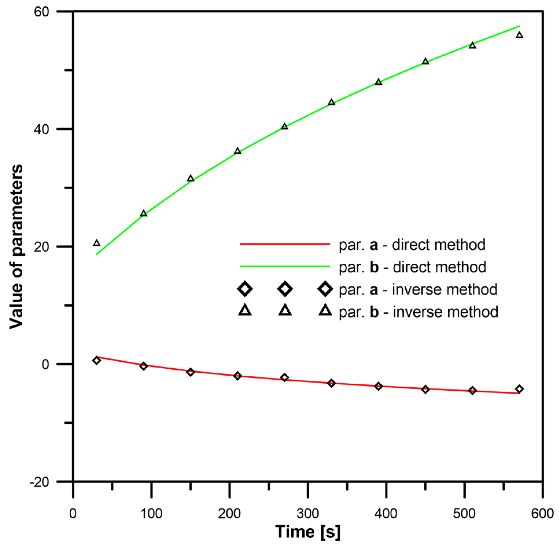Finally, the convective heat transfer varying both over time and along the plate length on the left boundary (h_mc (x, t)) was calculated. The heat transfer distribution in space was approximated using the following function

$$h_{mc}\left(x,t\right)=a\left(t\right)+b\left(t\right)/x^{0.5}$$

(13)

where parameters a and b were found by the least squares method in every minute of cooling. They are presented in

Table 1. Coefficients of the function approximating the distribution of the convective heat transfer in time and space in Equation (13).

t [s]	a [W/m2K]	b [W/m3/2K]
60	1.2198462	18.67917202
120	−0.162362	25.376006
180	−1.194652	31.048731
240	−2.005685	35.961097
300	−2.671	40.32
360	−3.238473	44.280206
420	−3.734243	47.914765
480	−4.181083	51.307252
540	−4.581333	54.476993
600	−4.955758	57.48656938

.

The temperature distribution during the cooling process was calculated using the FEM implemented in the ANSYS program [21]. ANSYS Mechanical APDL was used in the batch mode. The plate was discretized into 2000 linear plane finite elements. Ten elements were used along its thickness and 200 along its height. The convective boundary condition was assumed on the respective surfaces of 200 elements. The temperature histories obtained from the FEM were used as “exact measured data”. When the calculations were carried out with the time step of Δt = 60 s, the temperature distribution was very close to the one presented in [14], which was measured and generated by the MATLAB code. Figure 5 shows temperature transients f₁(t), f₂(t) and f₃(t) in points P₁, P₂, and P₃, respectively, whose location is given in mm based on the coordinate system in Figure 4: (3, 1), (62, 1), and (191, 1). A reduction in the time step to Δt = 10 s involved a slight difference in the temperature transients.

The unknown time- and space-dependent heat transfer coefficient of cooling in the mixed-convection regime was calculated by the proposed algorithm based on the three measured temperature transients f₁(t), f₂(t), and f₃(t) described in Figure 4.

It was assumed that the unknown parameters a and b from Equation (13) were functions of time. There were two unknown transients and three given measured temperature transients. Vector u_L consisted of two components: a(t_L) and b(t_L).

The temperature histories taken from the FEM with time step Δt = 10 s were considered as “exact measured data”. To obtain numerical tests similar to real conditions, “noisy measured data” were formulated by adding normal random errors of ±0.5 °C of the zero mean to “exact measured data” (σ_f = 1/6). These temperature transients in nodes P₁, P₂, and P₃ for the inverse solution are shown in Figure 6. They are compared to the data presented in the available literature [14].

The presented method was tested using the produced “noisy measured data” and time step Δt = 10 s. The values of <–10 W/m²K, 0 W/m^3/2K> and <10 W/m²K, 100 W/m^3/2K>, respectively, were chosen in vector u_L for the lower and the upper bound of all sought parameters. The starting vector was assumed as u_L(L = 0) = <1 W/m²K, 20 W/m^3/2K>. Calculations without future time steps could produce instability. To reduce oscillations, the number of future time steps was selected as N_F = 6. The number of iterations in each time step ranged between 3 and 30. If the midpoints of the constant parameter intervals were connected with straight lines, the estimated values of a and b were close to the exact ones as can be seen in Figure 7.

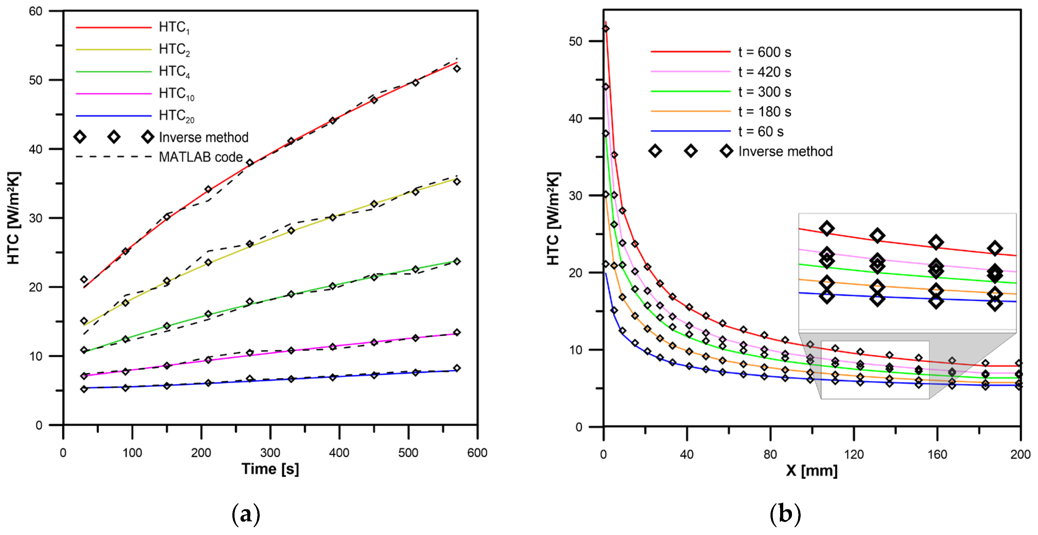
Finally, the unknown time- and space-dependent heat transfer coefficient distribution in the mixed-convection regime was calculated. The comparison between estimated and exact values is presented in Figure 8. The HTC transients in Figure 8a are shown for the following x coordinates: 1, 6, 16, 59, and 195 mm. They are also compared to the heat transfer coefficients calculated by the MATLAB code in paper [14]. It needs to be noted that in [14] twenty measurement points were used, and the investigation considered errors of ±0.1 °C. Despite the smaller number of measurement points and larger disturbance of measured temperatures than in [14], the obtained results were comparable. Additionally, the proposed method was easier to apply, as it allowed the use of commercial programs.

The introduced random errors had a slight effect on the identified boundary condition. Future steps effectively eliminated random measurement errors. During each iteration, the initial–boundary problem formulated by Equations (1)–(7) was solved by the FEM using the ANSYS software [21]. Due to the parametric formulation of the method, its use was simplified. The presented algorithm can be applied to transient nonlinear problems if they only have a direct solution.

4. Transient Analysis of Membrane Waterwalls in Steam Boilers

The furnace wall tubes are usually welded together using steel bars to make membrane wall panels, which are exposed to the furnace on one side and insulated on the other, as presented in Figure 9. A tubular-type instrument (flux tube) was installed to enable accurate measurement of the absorbed heat flux q_m and heat transfer coefficient h inside the membrane wall in steady-state conditions [22]. The proposed method was used to identify the absorbed heat flux and the heat transfer coefficient during transient operation.

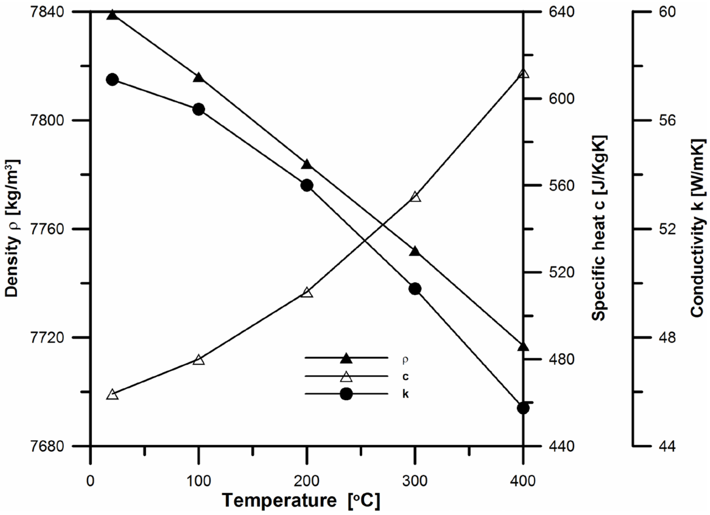
The membrane wall and the flux tube were made of 20 G steel. Temperature-dependent material properties were assumed (Figure 10). The following functions of the absorbed heat flux and of the heat transfer coefficient over time were assumed:

$$\begin{array}{l}\begin{array}{c}{q}_m\left(t\right)=14.03·t+\mathrm{39,038.8} \left[{\mathrm{W}/\mathrm{m}}^2\right]\\ h\left(t\right)=-1.12·t+\mathrm{14,970.9} \left[{\mathrm{W}/\mathrm{m}}^2\mathrm{K}\right]\end{array}\} \mathrm{for} 0<t<1000 \mathrm{s}\\ \begin{array}{c}{q}_m\left(t\right)=-1.025·t+\mathrm{53,068.2} \left[{\mathrm{W}/\mathrm{m}}^2\right]\\ h\left(t\right)=8.66·t+\mathrm{13,849.5} \left[{\mathrm{W}/\mathrm{m}}^2\mathrm{K}\right]\end{array}\} \mathrm{for} 1000<t<2000 \mathrm{s}\end{array}$$

Steam temperature totals T_m = 316.52 [°C]. The local heat flux on the membrane wall and on the flux tube was evaluated numerically using the FEM-based ANSYS program [21]. Due to symmetry, only the representative waterwall section presented in Figure 11 needs to be analysed. Temperature transients f₁, f₂, f₃, f_4, and f₅ in the locations illustrated in Figure 9 were calculated using the FEM and disturbed with normal random errors ±0.5 °C of the zero mean (σ_f = 1/6). The generated “noisy measured data” for the inverse solution are shown in Figure 12.

There were two unknown transients q_m(t), h(t) and five given measured temperature transients. Vector u_L consisted of two components: u₁(t_L) and u₂(t_L).

The proposed method was tested with the time step of Δt = 10 s. The values of 0 and 100,000 <W/m² K, W/m²>, respectively, were chosen in vector u_L for the lower and the upper bounds of the sought parameters. The starting vector was assumed as u_L(L = 0) = <15,000 W/m²K, 40,000 W/m²>.

To reduce oscillations, the number of future time steps of N_F = 20 was selected. The number of iterations in each time step ranged between 1 and 8. The estimated boundary conditions were close to the exact values, as can be seen in Figure 13.

5. Conclusions

The presented survey of the up-to-date state of knowledge indicated that despite the great number of works devoted to the issue in question, there was no simple method, which allowed the use of commercial programs for the identification of the transient thermal state in elements with a simple or complex shape. The proposed method did not require writing the source code with the use of FDM, CVM, or FEM. Its advantage was the possibility of using commercial programs. In this work, the ANSYS software using the FEM was applied. The two presented examples demonstrated good stability and accuracy of the developed method. The proposed inverse method made it possible to estimate the convective heat transfer coefficient in the heated vertical plate varying both in time and space during cooling under the mixed-convection regime. Despite the smaller number of measurement points and greater disturbance of measured temperatures than in [14], results comparable to [14] were obtained. The developed iterative algorithm was also applied to estimate the time-dependent heat flux and the convective heat transfer coefficient in the steam boiler membrane waterwall. The analysed component had the form of the non-simply connected domain Ω, and temperature-dependent thermophysical properties were assumed. Calculations were performed for the unknown heat flux or the heat transfer coefficient distribution on the domain boundary based on measured temperature transients disturbed with the random error of 0.5 °C. To reduce oscillations, the number of future time steps of N_F = 20 was selected. The number of iterations in each time step ranged between 1 and 8. The estimated boundary conditions were close to the exact values. The method can be used in practice in an offline mode.