Energy Cell Simulation for Sector Coupling with Power-to-Methane: A Case Study in Lower Bavaria

Abstract

In this study, the possibility of sector coupling with biological Power-to-Methane to support and stabilize the energy transition of the three major sectors of electricity, heat, and gas was addressed. For this purpose, the energy cell simulation methodology and the Calliope tool were utilized for energy system optimization. This combination provides detailed insights into the existing dependencies of consumers and fossil and renewable energy suppliers on a local scale. In this context, Power-to-Methane represents an efficient technology for quickly and effectively exploiting unused electricity potential for various sectors and consumers. It was found that, even in regions with low wind levels, this surplus electricity potential already exists and depends on various influencing factors in very different ways. The solar influence on these potentials was considered in connection with gas-fired cogeneration plants for district heating. It was found that the current heat demand for district heating produces a large amount of electricity and can generate surplus electricity in the winter. However, in the summer, large amounts of usable waste heat are dissipated into the environment, owing to the low consumption of district heat. This problem in the heat sector could be reduced by the expansion of photovoltaics, but this would require further expansion of storage or conversion systems in the electricity sector. This demonstrates that the consideration of several sectors is necessary to reflect the complexity of the sector coupling with Power-to-Methane properly.

1. Introduction

According to the Intergovernmental Panel on Climate Change [1], a limited CO₂ budget remains for the world to achieve the global goal of limiting the maximum temperature increase to 1.5 °C. With an estimated budget of 580 GtCO₂ remaining to emit, the goal will be achieved by 50%. This goal of only emitting 580 GtCO₂ can only be achieved through further expansion of renewable energy and storage systems. In Europe, countries such as Germany have committed themselves to reducing greenhouse gas emissions by up to 100% by 2045 compared with their 1990 levels. Since 1990, 40.8% has been achieved in Germany [2]. This massive emission reduction and the reduction that still has to be done indicate the urgency of the situation.

Reducing emissions does not only result in changes in the electricity sector, where renewable energies have advanced most visibly. It is becoming increasingly important to increase the use of renewables in the transport and heat sectors. The transport sector is currently undergoing a change owing to technological advances in battery development and public policies. In the heat sector, which is the second-largest CO₂ emitter in Germany, policies have been developed to reduce energy consumption. Strategies include switching from fossil fuels to renewable sources, such as from coal to renewable natural gas (RNG), switching content (meaning increasing the amount of RNG), and employing the so-called “modal switch” [3] (turning, for the most part, to decentralized structures in the heating sector, as well as renovation and optimization of decentralized heating systems). One of the most important strategies of the modal switch is district heating. In this context, to provide a means of storing energy, clean heat sources, and solutions for the transport sector, technologies such as Power-to-Methane (PtM) can help in solving these problems [4,5,6,7]. PtM technologies are essential for the production of RNG, which can be fed in the natural-gas grid. In the first power-to-hydrogen step, water is separated into hydrogen and oxygen through electrolysis, either via alkaline (AEL) or the polymer electrolyte membrane (PEM). AEL has long been used in hydrogen production and, therefore, is already applicable on a large scale [5]. PEM has a more flexible and faster load behavior. Thema et al. [4] reviewed several implemented projects and came to the conclusion that, despite AEL having a better CAPEX due to the long experience, AEL and PEM are implemented in approximately equal shares. In the second hydrogen-to-methane step, the produced H₂ reacts with CO₂ to CH₄. Either chemical-catalytic or biological methanation is available for this purpose. Graf et al. [6] showed that catalytic methanation is more efficient but also has less flexibility in the load change behavior. Biological methanation, on the other hand, has much more moderate reaction conditions and resistance to gas contamination [8]. The projects investigated by Thema et al. [4] show that catPtM has so far achieved higher maximum capacities and also has better CAPEX than bioPtM. However, both technologies are implemented approximately equally often. As discussed by Morgenthaler et al. [7] the combination of battery and PtM is a novel concept to make energy surplus more accessible.

The increased expansion of renewable energy sources (RESs) to cover these demands has led to several problems in the power grid, challenging its current centralized structure. Among the several issues affecting the grid, peak shaving, where industrial and commercial power consumers level out their peaks in electricity use, and electricity surpluses that arise at times of high renewable energy supply pose the biggest problems. In response to these demands, it is necessary to develop approaches that involve a greater number of stakeholders, as has been proposed for different circumstances [9] and approaches to energy transitions [10]. At the center of these new approaches, a new generation of prosumers are active in the energy system, with the expectation that new democratic forms of citizen participation will emerge [11]. However, it is important to establish the extent to which different technologies and types of demand can be efficiently combined at the local level [12]. Establishing a regional and local planning system is of great relevance because energy markets (bidding zones) are usually national or supranational. Because of the oversupply of electricity, its stock market price can fall to such an extent that negative electricity prices are sometimes generated [13]. To reduce the surplus, either conventional power plants must be shut down or the production of renewable energy must be curtailed.

For predicting power surpluses and placing storage technologies in the power grid, complex simulations must perform at the local level. However, this requires a significant amount of knowledge about the area to be modeled and specific simulation tools [12]. Normally, the simulation of energy systems is carried out at an industry level and restricted to a few industrial processes or buildings, or it is at the level of entire regions or countries based on aggregations of demand and generation [14]. However, a new generation of simulation tools makes it possible to realize multi-nodal simulation models at different geographic and temporal scales [15,16]. This makes the development of meso-level simulations in clearly defined regions possible, simulating their respective interrelationships. In these so-called “energy cell simulations”, the influence of the deployment of storage technologies and distributed generation on energy cells [17] can be considered over several years [7].

Energy cells are defined here as a self-defined geographic scale, which usually consists of buildings, neighborhoods, or cities. Scaling can also be up to the national scale. For example, Tröndle et al. [18] pointed out that 497 energy cells were defined for the “Fully Renewable Electricity European” Calliope model. Some studies subdivide cities into different sub-energy cells, which are connected to specific local electricity load and supply profiles [15]. The cellular approach that inspired this study makes it possible to transmit the energy that is not used in certain identified energy cells to cells that cannot guarantee their own supply because of weather phenomena or high energy consumption. In other words, energy should be consumed where it is generated, or it should be transported to the energy cell that needs energy.

1.1. Research Problem

In the literature on regional energy system simulations, weather data has proven to be an important issue in various contexts [19]. There is also great concern about the quality of the data used to develop power system simulation models that serve as the basis for decision-making [20]. In this regard, much effort has been devoted to the improvement and validation of new climate data collections [19]. Several re-analysis data studies show that some sources are different but, in some cases, may not have a significant impact on the resulting simulation models [21].

Regarding the geographical dimension, because of the lack of granular data on the geography, location, and demand loads, researchers and institutions have filled this gap by developing databases that offer an aggregated or typical view of the daily behavior of a consumer (Standard Load Profiles or SLP), the typical annual consumption of different consumers, and the consumption in a region based on the top-down calculations based on economic activities [22]. These databases are usually developed from disaggregation of data by class, and they do not always coincide with reality [23].

In this study, we tackle this issue from a bottom-up perspective, with relatively few simplifications, rather than a strictly top-down perspective. Moreover, as SLP data can be inaccurate, standard consumer profiles were compared with real data collected in the two case study regions. This makes the study highly valuable for real-world applications for future investments in the field of energy storage.

Another subject that has not been investigated sufficiently is the storage of renewable energy via PtM and the resulting heat generation [24]. Wind and PV produce renewable power, but what is needed is the transformation into storable energy resources that can be transported and distributed in existing energy grids and that can be used in the transport and heat sector. PtM offer opportunities that are currently not integrated into energy simulation models [25].

1.2. Research Objective

This article presents the results of two optimization models for two case study regions in Germany. The optimization models simulate all available generation sources available in the regions and their extension with an additional PtM technology. The optimization model minimizes the cost of the overall systems that meet the given demand to determine which combinations of technologies are economically meaningful.

The working hypothesis is that the use of real demand profiles (RLP) combined with multiple time series of weather data should have an impact on the economic results of the optimization model compared to models using only a one-year data series and SLP. Therefore, we optimize the size of the systems using SLP [20], a demand that is characterized by no large peaks of use and very regular behavior, and compare them to the results of RLP, which contains a larger amount of variation. Our analysis focuses on runtime and size capacity because the use of RESs and energy storage technologies depend highly on peak demand and production. This should be especially visible in energy-conversion technologies, such as PtM.

To control for the impact of these two demand curves on the simulation results, five years with their respective solar data were considered. This makes it possible to control for the level of influence of using multiple years of weather data in the existing photovoltaic generation sources. This should control for possible “cherry-picking” strategies regarding weather data and electricity usage.

Instead of focusing only on electricity generation, heat, or gas [26], we included RLP and SLP for natural gas demand, electricity demand, and heat demand. Efficient technologies to provide heat and power are combined heat and power (CHP) technologies. When CHP plants are operated to produce heat on demand, sometimes there is surplus electrical power. When they are operated to fill shortages in the provision of electrical power, sometimes there is surplus heat. PtM produces additional heat, mostly in the process of electrolyzing renewable power from wind or PV. This work evaluates the system-supporting role of biological PtM in the field of decentralized gas and district heat grids and efficient energy production, conversion, and use in an energy cell.

2. Materials and Methods

In the following, the simulation in this study is explained. In addition, the different data used, as well as the process carried out for their collection, preparation, and use, are presented.

First, we identified the energy demand for heat, electricity, and gas by type of consumer. For that, data on electricity, heat, and gas hourly load profiles were collected for different exemplary categories according to their sector of activity from the district heating and distribution companies working in the region. Second, to identify the weight of each category in the total energy demand, final users’ size and number were identified using building categories from OSM data. For that, OSM data were classified according to their size and location and assigned to the demand profiles, which were normalized based on public estimates of annual regional energy consumption. Third, the characteristics of the available energy generation plants were included based on the Bavarian Energy Atlas [27]. Here, generation technologies such as renewable energy systems (RES) such as hydropower were used, but fossil-fuel-based combined heat and power generators were also included. Then, a mixed linear-integer program (MILP) to define the size of the PtM system that minimizes the overall cost of the regional energy system was proposed. Finally, the MILP was applied to the two case studies for two different scenarios in different years. Nevertheless, providing optimal system sizing based on all available energy sources was beyond the scope of this study.

2.1. Optimization Model

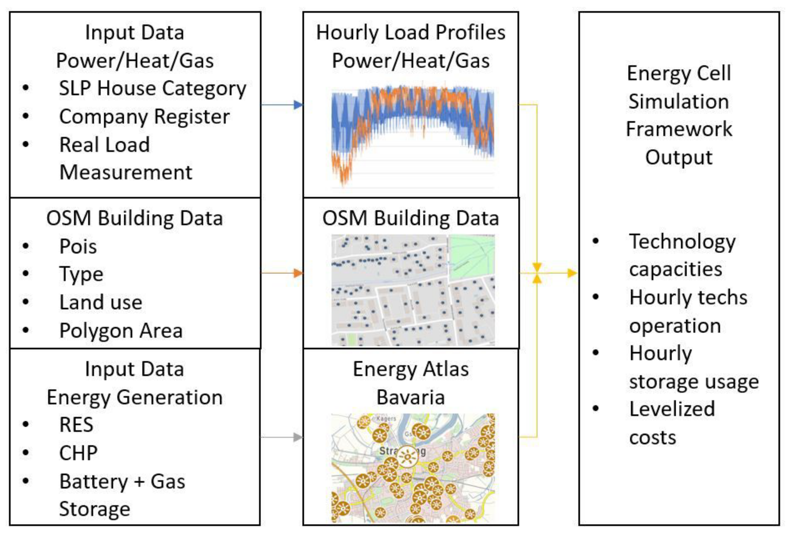
In this paper, we continued the mixed-integer linear optimization (MILP) model from Valdes et al. [20] with hourly resolution and analysis of the hourly operation of generation and storage, such that the electricity demand in different periods was met. In this article, we considered two case study regions with a PtM system coupled to its renewable and other existing non-electricity supply technologies. The applied modeling framework computed the optimum PtM system size and operation for a given predefined demand of electricity, gas, and heat. The model calculated the amount installed capacity required to produce a certain demand at each time step t and a certain total accumulated demand for every period p. The model resembled others, such as the model presented by Pfenninger and Keirstead [28] and the model presented by Díaz et al. [29]. One main difference is that this model presented, in addition to an electricity demand, an added heat and gas demand.

The optimization model was developed using the Calliope modeling framework. Calliope is an open simulation framework for optimizing and simulating energy systems, including different energy carriers. The details of the optimization model and the different constraints and conditions were not described. These can be found in Pfenninger and Pickering [30] and in Pontes Luz and Amaro e Silvia [31], as well as in subsequent applications. In general terms, the objective of the model presented here was to minimize the overall costs necessary to cover the electricity and heat demands of each region, which was the result of the aggregation of seven building categories, using a limited number of available technologies. A simplified model is shown in Figure 1.

The power, heating, and gas demand is the aggregate demand of different types of users classified according to their consumption profiles [32,33] (see Appendix A). Heat was generated with the CHP and PtM technologies. The PtM technology allows for supplying the heat and gas sectors with renewable methane gas. In addition, with the use of CHP technologies, electricity and heat are generated simultaneously to cover the estimated district heating demand. The CHP power plants are fired exclusively by gas, which can be covered by the PtM plant, or by the gas grid supply, which is unrestricted. The model included the investment costs, production, and operating and maintenance (O and M) costs for each technology [7,34,35]. The use of PV and hydropower technologies was forced. This means that these sources are always first activated to meet the demand and the hourly potential was fully utilized. This priority over all others potentially results in excess energy.

We used Calliope in a model in which only three hypothetical sub-regions were considered: one region representing the generation sector, another including energy conversion and storage technologies, and a last one including all energy demands (demand, heat, and gas). This did not represent a real system such as other previous applications involving multiple energy carriers [31,36], but the location and characteristics of the grid were not available at the distribution grid level, therefore distribution grid losses may be not representative.

The simulation framework Calliope has been identified as one of the most flexible frameworks, and together with oemof and urbs, it is the only framework capable of including a multi-energy system perspective, owing to its capacity to include different energy carriers and sources [14]. The full mathematical formulation of the framework is available online [37]. As in previous research [7], a PtM plant coupled to its own renewable electricity supply technologies was considered, but other existing technologies and the possibility of drawing gas from the grid was included in this case. The input parameter values used are summarized in

Table 1. Techno-economic model input data.

	Installed Capacity SR [kW]	Installed Capacity VOF [kW]	Investment Cost [€/kW]	Consumption Cost [€/unit]	Fix O and M [€/kW]	Lifetime [a]	Efficiency	Min. Usage of Capacity [%]
Hydropower	21,500	5000	5250	0	52.5	80	0.85	100
PV	54,028	24,517	1050	0	10.5	25	0.90	100
CHP bio	1354	4780	3000	-	30.0	20	0.35	0
CHP 65 MW	65,000	65,000	787.5	-	15.57	25	0.332	0
CHP 22 MW	22,000	22,000	400	-	0.005	25	0.46	0
PtM	Infinite	Infinite	4568	-	137	25	0.54/0.85	0
Battery	5403	2452	1028	-	25.19	11	0.90	0
Gas pipeline	Infinite	Infinite	0	0.016	0	50	1.00	0
Bio supply	Infinite	Infinite	0	0.03	0	50	1.00	0
H2O supply	Infinite	Infinite	0	3.27	0	25	1.00	0
CO2 supply	Infinite	Infinite	0	0	0	25	1.00	0

Infinite: No limitations for calliope to optimize the scale of the technology.

.

2.2. Input Data

The data used in this study came from various sources, including newly collected end-use energy hourly consumption data for electric and thermal clients; meteorological data for the PV panel simulation from renewables.ninja [38], such as in Pfenninger and Staffell [39]; public data on annual energy consumption data per region [27]; geographic data on the building usage [40]; public data on existing generating units and power plants [41]. These data are presented in Section 2.1. The methodology consisted of three phases, following Valdes [20] and Alhamwi [15], as shown in Figure 1.

2.2.1. Energy Generation and Sources

The generation side consisted of a combination of public available installed capacities that were available in 2020 in the locations considered and a set of potential technologies. All RESs used in the simulation are available from official sources [27]. These are PV, hydropower, and biogas plants. The installed maximum capacity of the available technologies is listed in Table 1. To make full use of renewable electricity, hydropower and PV generation capacities were always fully utilized and no curtailment was necessary. Time series weather data for PV were collected from Pfenninger and Staffell [39]. They offered bias-corrected capacity factors for renewable energy systems for PV over different years. To cover the electricity and district heating demand in times of need, conventional gas-fired CHP technologies were available. These CHP plants were not directly located in the region, but the current CHP plants are present in the vicinity. The CHP plants are, besides PtM, the only heat source for district heating demand. In addition to the methane produced by PtM, natural gas was sourced from the German gas grid, and the cost and gas composition were the same as in the German gas mix in 2019. Natural gas is available to cover direct demand from CHP and households.

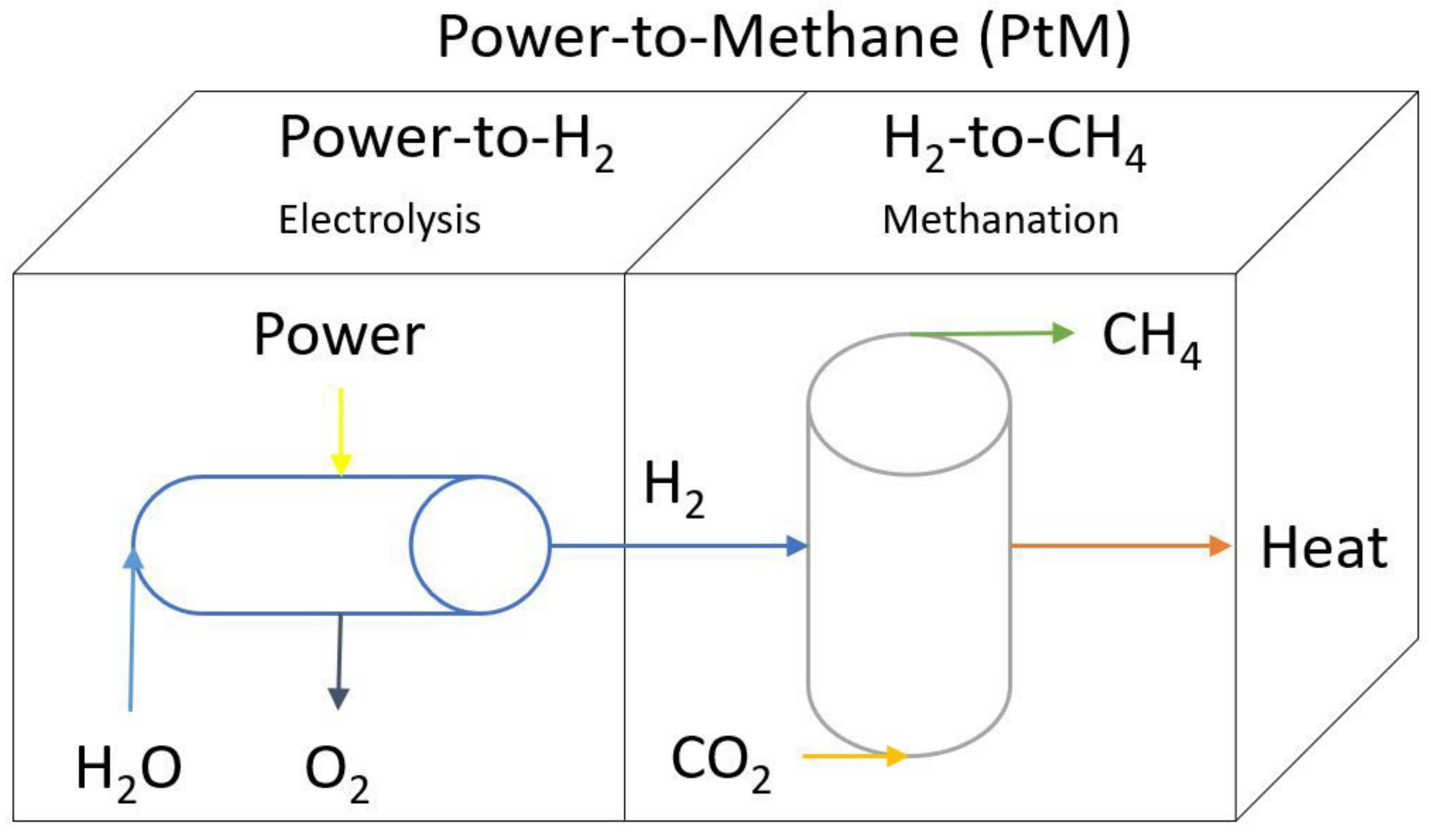
2.2.2. Energy Conversion and Storage

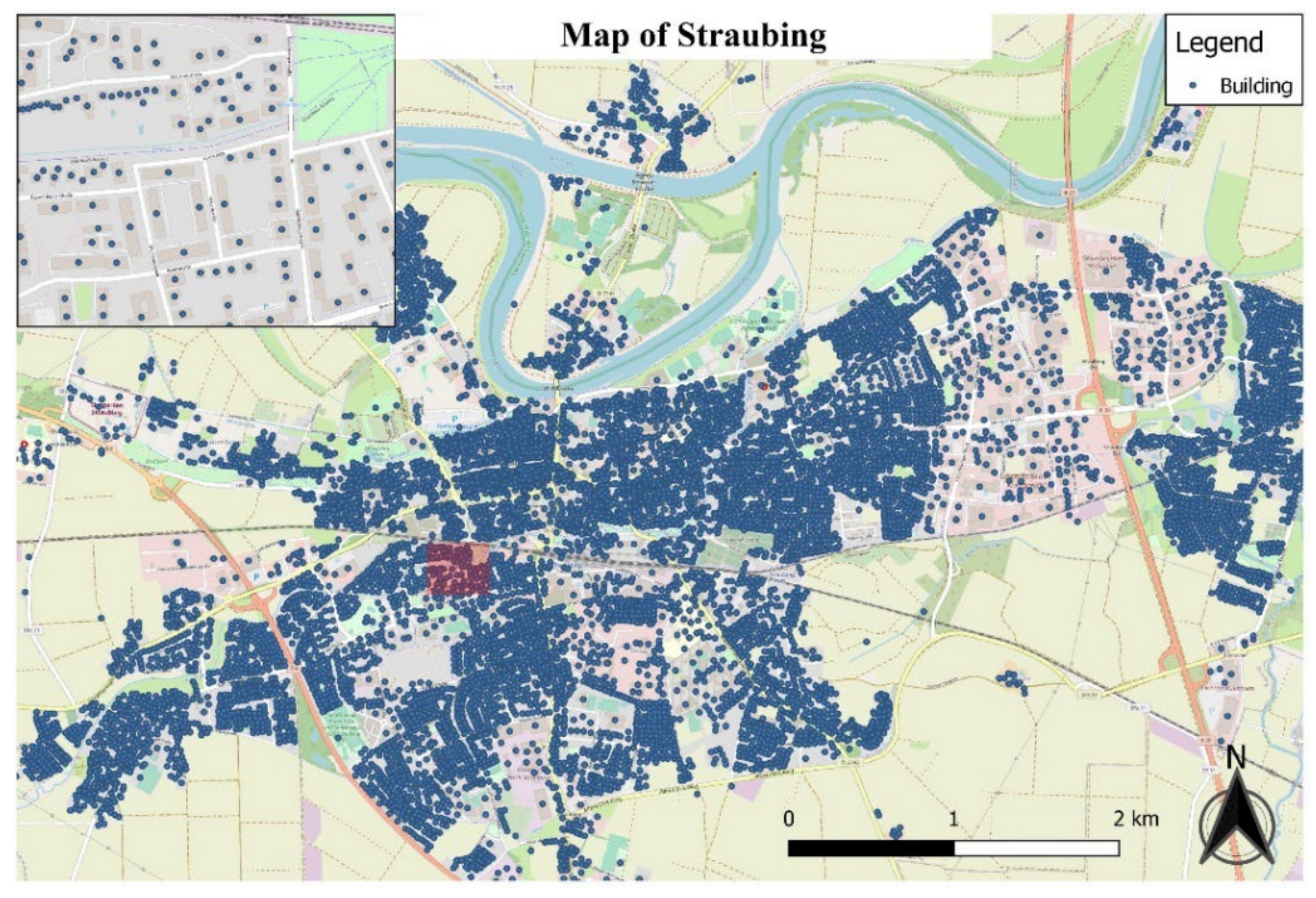
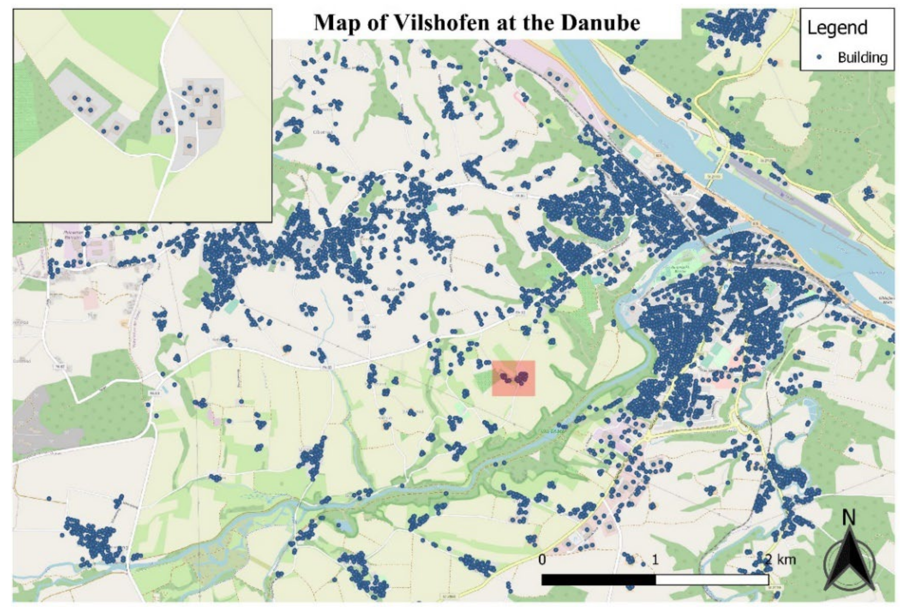
In the model, battery storage was first assumed, which corresponded to 10% of the PV power installed on each case study region. This enabled the battery to compensate for smaller power surpluses, which would still be too small for a PtM system to ramp up. In addition, the battery can be charged or discharged to 25% within one hour. Other values necessary for the simulation were taken from a market survey for battery storage [42] (p. 20).

A simplified PtM model (see Figure 2) was calculated following Valdes et al. [20]. For the PtM technology, it was considered that electrolysis is not carried out separately and that all hydrogen can be directly transformed into methane. The upper heating value for H₂ was 3.54 kWh/Nm³, and for CH₄, it was 11.06 kWh/Nm³. As the study reviewed electrical surplus with lots of start and shut-down cycles, we chose a PEM electrolyzer for the flexible load behavior. The nominal H₂ production for a PEM electrolyzer was given by H-Tec [43], with 0.22 Nm³/h at an electrical nominal load of 1 kWh for the S-Series in relation to the upper heating value. This led to an efficiency factor of 78%, which was close to the average value determined by Thema et al. [4] for hydrogen projects implemented.

4 H₂ (g) + CO₂ (g) → CH₄ (g) + 2 H₂O (L)

(1)

The thermo-dynamical efficiency achievable by methanation in relation to the upper heating value regarding the Equation (1) was 78%. Graf et al. [6] stated that the efficiency factor is further influenced by own electrical and heat consumption and give a range for electrical own consumption of 0.4–1.8 kWh/m³ _SNG for biological methanation. In this study, biological methanation was assumed due to its flexible load cycling characteristics and robustness to gas impurities. This allowed for us to easily use digester gas from the digester towers present in the wastewater treatment plants without additional gas cleaning. In addition, biogas from biogas plants could be used for upgrading. The whole PtM plant was assumed conservatively with an electrical energy requirement of 11% of an available electricity surplus for pumps, heating, and supporting systems. This means that a power input of 100 kW led to 89 kW for electrolysis and 11 kW for methanation and supporting systems. This led to an output of 0.539 kW methane per 1 kW of power input and lowered the overall efficiency of bioPtM to 53.9%. This value was in line with the efficiency value of 54% for bioPtM reported by Götz et al. [5] and Graf et al. [6]. The by-product oxygen and the input of water for the electrolysis were calculated, but only the water consumption was monetized. Nevertheless, the cost of water was minimal, so the influence on the economic performance of the PtM plant was negligible.

The amount of CO₂ needed for the methanation was also calculated, but because the investigated regions had biogas plants and digesters at the sewage plant for biogas upgrading, it was assumed that the required CO₂ was provided cost-neutrally by those. Trading CO₂ certificates could generate income with CO₂ consumption. However, if no nearby sources are available, then CO₂ consumption can generate costs. The waste heat produced during the electrolysis and methanation was directly set to the usable standard value of 80%, as published by Friedl [44].

2.3. Case Studies

SR is a city with approximately 48,000 inhabitants and is compactly populated (see Figure 3). VOF, with approximately 16,000 inhabitants, is considerably smaller than SR and is more of a sprawling rural region (see Figure 4). Both regions have diverse renewable energy production but lack wind power. They were chosen because they contain an industrial area that includes an energy-intensive enterprise. As in a previous report [20], they may present an opportunity to develop energy communities or other infrastructure development between existing industries and nearby urban residential areas. Instead of using data from official sources, following Alhamwi [45], the model input data were based on the open-source OSM data and consumption data for 2019. OSM is often used for geographic information system (GIS) modeling, spatial analysis, or statistics. OSM data were obtained from Geofabrik GmbH. It was already proven by the work of Alhamwi et al. [46] that the quality and availability of OSM data meet scientific requirements and are comparable to commercial geodata.

The available OSM data were processed according to Valdes et al. [20] to determine building classes and their number in the considered districts, SR and VOF (see Appendix A). In this process, the building roof polygons were transferred to points in the averaged building centroids. Buildings were assigned directly to building classes according to the type and POIs classifications available in the OSM data. If this was not possible, an assignment was made using the land-use category and polygon roof area.

2.4. Scenarios

PtM and battery system size were calculated for 30 different scenarios for SR and VOF, where two sets of demand profiles were considered and the study period was modified, as well as the modification for PtM. In the case studies, the period from 2015 to 2019 was examined for SR and VOF to investigate the influence of weather data. The overall consumption of the building categories for electricity and heat was always the same. Similarly, the technologies were kept the same for all simulations, and only the PtM varied for three scenarios. In the first variant, the PtM was not used to investigate the effect on the use of the gas grid. The second variant used PtM without a gas grid connection so that there was no storage option for the gas produced and it had to be directly used. The third variant was simulated with the gas grid connection as a storage option. In addition, we optimized the system size using the SLP and RLPs for the same periods (see Appendix B).

Load profiles are necessary to calculate the demand for electricity, gas, and heat from consumers in simulations. In principle, load profile data can be requested from network operators or companies, but companies do not provide the data lightly because the data are sensitive. Within this study, cooperation agreements were concluded with several companies to be able to use their data in the simulation. Additionally, standard load profiles (SLPs) for electricity and gas were created by BDEW [32,33]. SLPs were used to analyze the load behavior of consumers without power metering and to make predictions about the consumption behavior of different customer groups [47] (p. 379). The SLPs were divided into different consumer groups with different load behavior. There were residential, commercial, agricultural, and industrial groups based on SLPs.

Standard and Real Load Profiles

The building classifications shown in

Table A1. Annual energy demand by building category for Straubing and Vilshofen.

B. Class		Definition	Building	Demand	Demand	Demand	Demand	Building	Demand	Demand	Demand	Demand
SLP	SLP	Building	SR	H SR	G SR	D.H SR	P SR	VOF	H VOF	G VOF	D.H VOF	P VOF
P	G/H		[n]	[MWh/a]	[MWh/a]	[MWh/a]	[MWh/a]	[n]	[MWh/a]	[MWh/a]	[MWh/a]	[MWh/a]
H1	GHEF03	Detached house	6985	87,899	42,192	12,306	47,484	5081	63,939	30,691	8952	16,208
H2	GHMF03	Apartment building	3417	94,104	45,170	13,175	23,229	2557	70,420	33,801	9859	8156
G1	GGMK03	Business weekdays 0800–1800	598	172,368	82,736	24,131	54,321	171	49,289	23,658	6900	21,877
G2	GGGA03	Business evening	38	9964	4783	1395	3452	8	2098	1007	294	1023
G3	G0	Business 24/7	243	43,488	20,874	6088	22,074	57	10,201	4896	1428	7292
G4	GGHA03	Trade	9	468	225	66	818	2	104	50	15	256
G5	GGBA03	Bakery	2	227	109	32	182	0	0	0	0	0
G6	G0	Business weekend	28	5011	2405	702	2543	17	3042	1460	426	2175
BI	GGKO03	Industry	139	234,350	112,488	32,809	139,426	42	70,811	33,989	9913	51,560

(see Appendix A) were based on the BDEW [22], Schröder et al. [48], and the assumptions in this study. The BDEW classification must be adapted for various reasons. The segregation of classification H0 follows Schröder and, therefore, has been extended into single-family houses (H1) and multifamily houses (H2). The big industries (BI) profile is one of the most important categories because it reflects the energy-intensive industrial sector. The profile contains all buildings with very high electricity consumption [20]. Most buildings in the BI profile cannot be divided into G1-G6 because they are no longer SLP customers but RLM customers. In addition, a class for small buildings with zero demand was introduced, which is not listed in Table A1. This class included garages, barns, or buildings under a specific roof area for each class to minimize the error in the building number. The building classes based on SLP electricity were assigned to the corresponding SLP gas. These gas profiles were also provided by the BDEW [32] (p. 144), [49]. Because no unique SLP gas was available for G1 and BI, a correlation calculation was used to assign the best matching SLP gas. Because no data on annual gas consumption were available for profiles G6 and G3, profile G0 was created. This profile was obtained from a summary of the available group profiles.

The BDEW did not provide SLPs for heat. Schellong [47] (p. 379) explains that the SLPs for gas are based on the heat demand of consumer groups. Since natural gas in the area of SR and VOF is mainly used for building heating, the SLP gas was used in this study to create heat load profiles. Various examples are provided in the literature on how heat load profiles can be created. Ruhnau et al. [50] created heat load profiles for different countries in Europe, consisting of hourly data, to compare them with the coefficient of performance time series of heat pumps and to improve their efficiency. Schüler et al. [51] referred to data from the Canton of Geneva in Switzerland for the development of heat profiles, which provides a great deal of publicly available information for the entire building sector. The available data were divided into different building categories, and regression analysis of different parameters was used to develop heat demand projections. In this study, the heat load profiles were calculated using SLP gas in combination with the efficiency factor of 0.98 of a gas condensing boiler.

3. Results

The total annual electricity demand needed to generate the Load Profiles was provided by the Bavarian State Ministry [27]. Class-specific demand ratios were then determined using the respective building areas. The annual heat demand was determined using anonymized annual consumption data for gas and district heating from the SR and VOF municipal utilities. For a given district heating consumption, losses during heat transfer were neglected, as neither the topology of the grid nor current measurements were available. Because different building types were included in the commercial profiles, the annual consumption was averaged over all included buildings of each class. The total heat demand was then calculated according to the percentage distribution of heating type for private dwellings in Germany, as determined by the BMWi [52] and BDEW [53] (p. 23). Therefore, 48% of the total heat demand was transferred to the gas demand for heating, and 14% was used for the district heating demand. For this study, not the heat sector in general but the gas and district heating sectors were of interest because PtM has an input potential there. As a result, Figure 5 shows the annual energy demand in MWh. The gas consumption consisted of the amount consumed in private households for heating. Figure 6 shows the distribution of energy demand among the building classes, while Figure 7 contains the general building distribution of the regions. Here, it became clear that even a few big industrial buildings have a large impact on the energy consumption of the region.

Figure 8, Figure 9, Figure 10 and Figure 11 show the exemplary course of the demand curves for electricity and heat from the 1–7 February 2019, a typical winter week. They show that the electricity demand (in kWh) was significantly lower on weekends than the average weekly consumption. As Figure 8 and Figure 9 show, by prioritizing the use of the RESs, heat demand led to an excess of electricity generation in the winter. The proposed model reduced the use of existing fossil power generation by giving priority to RES sources because of the regulations in Germany that renewable power generation is preferred over fossil power generation [54]. The optimization model first activated the renewable electricity generation sources to meet the electricity demand. To meet the heat demand (Figure 10 and Figure 11), the CHP plants were activated, producing heat and electricity. As the demands are not the same and some technologies generate heat and/or electricity, heat and electricity sources can generate a surplus. In the case that more heat than necessary is produced, the excess is released into the environment. The electricity surplus is stored in a battery and/or converted to methane in the PtM. The methane production by PtM, in turn, can be used to meet gas demands. The difference in the resulting hourly demand between SLP and RLP is best seen in Figure 8 and Figure 9. The red line represents the electricity demand showing more irregularity and more consumption peaks.

3.1. Results for Standard Load Profiles

Table A2. Simulation results for standard load profiles in Straubing without PtM.

Year	Power	PV	Power	Battery	Power	Gas Grid
	Surplus	Runtime	Output	Runtime	Output	Output
SLP	[MWh/a]	[h]	[MWh/a]	[h]	[MWh/a]	[MWh/a]
2015	62,167	4390	56,625	2724	3401	603,269
2016	60,837	4367	53,691	2749	3349	606,163
2017	61,789	4380	55,053	2767	3385	605,389
2018	60,944	4379	54,895	2754	3407	603,783
2019	60,652	4379	55,047	2820	3429	603,292

,

Table A3. Simulation results for standard load profiles in Straubing without PtM stored.

Year	Power	PV	Power	Battery	Power	Gas Grid	PtM	Power	Gas	Heat
	Surplus	Runtime	Output	Runtime	Output	Output	Runtime	Input	Output	Output
SLP	[MWh/a]	[h]	[MWh/a]	[h]	[MWh/a]	[MWh/a]	[h]	[MWh/a]	[MWh/a]	[MWh/a]
2015	52,338	4390	56,625	2726	3300	552,237	4005	−51,579	27,816	16,017
2016	51,286	4367	53,691	2730	3240	552,119	3953	−50,541	27,257	15,695
2017	51,922	4380	55,053	2814	3273	553,189	3984	−51,169	27,596	15,890
2018	51,090	4379	54,895	2866	3290	555,054	3946	−50,333	27,145	15,630
2019	50,941	4379	55,047	2744	3320	550,905	4031	−50,178	27,061	15,582

,

Table A4. Simulation results for standard load profiles in Straubing with PtM stored.

Year	Power	PV	Power	Battery	Power	Gas Grid	PtM	Power	Gas	Heat
	Surplus	Runtime	Output	Runtime	Output	Output	Runtime	Input	Output	Output
SLP	[MWh/a]	[h]	[MWh/a]	[h]	[MWh/a]	[MWh/a]	[h]	[MWh/a]	[MWh/a]	[MWh/a]
2015	51,078	4390	56,625	2796	3331	549,177	3996	−50,312	27,133	15,623
2016	50,050	4367	53,691	2742	3276	553,358	3949	−49,296	26,585	15,308
2017	50,809	4380	55,053	2783	3313	551,665	3981	−50,047	26,990	15,541
2018	49,981	4379	54,895	2772	3329	550,598	3943	−49,215	26,541	15,283
2019	49,865	4379	55,047	2821	3348	550,762	4016	−49,095	26,477	15,246

,

Table A5. Simulation results for standard load profiles in Vilshofen without PtM.

Year	Power	PV	Power	Battery	Power	Gas Grid
	Surplus	Runtime	Output	Runtime	Output	Output
SLP	[MWh/a]	[h]	[MWh/a]	[h]	[MWh/a]	[MWh/a]
2015	17,705	4381	24,628	2491	1381	263,116
2016	17,057	4368	23,507	2465	1375	263,938
2017	17,617	4383	24,073	2480	1383	263,931
2018	17,070	4376	23,884	2541	1386	263,041
2019	17,136	4385	24,087	2494	1378	263,040

,

Table A6. Simulation results for standard load profiles in Vilshofen without PtM stored.

Year	Power	PV	Power	Battery	Power	Gas Grid	PtM	Power	Gas	Heat
	Surplus	Runtime	Output	Runtime	Output	Output	Runtime	Input	Output	Output
SLP	[MWh/a]	[h]	[MWh/a]	[h]	[MWh/a]	[MWh/a]	[h]	[MWh/a]	[MWh/a]	[MWh/a]
2015	14,382	4381	24,628	2531	1334	247,239	3462	−14,074	7590	4370
2016	13,883	4368	23,507	2497	1331	248,706	3449	−13,576	7322	4216
2017	14,286	4383	24,073	2507	1332	248,123	3488	−13,979	7539	4341
2018	13,825	4376	23,884	2521	1344	247,708	3437	−13,515	7289	4197
2019	13,828	4380	24,087	2507	1329	247,631	3479	−13,521	7292	4199

and

Table A7. Simulation results for standard load profiles in Vilshofen with PtM stored.

Year	Power	PV	Power	Battery	Power	Gas Grid	PtM	Power	Gas	Heat
	Surplus	Runtime	Output	Runtime	Output	Output	Runtime	Input	Output	Output
SLP	[MWh/a]	[h]	[MWh/a]	[h]	[MWh/a]	[MWh/a]	[h]	[MWh/a]	[MWh/a]	[MWh/a]
2015	14,178	4381	24,628	2502	1412	247,087	3318	−13,489	7275	4189
2016	13,673	4368	23,507	2499	1418	248,522	3323	−12,983	7002	4032
2017	14,117	4383	24,073	2490	1411	247,969	3344	−13,429	7242	4170
2018	13,675	4376	23,884	2516	1420	247,567	3264	−12,983	7002	4032
2019	13,685	4380	24,087	2472	1411	247,471	3346	−12,997	7010	4036

in Appendix B show the aggregated results of the SLP simulations of SR and VOF. As we were interested in the use of conversion and storage technologies, we reported here an overview of these technologies and associated metrics.

The first scenario served as a first assessment of the resulting electricity surplus potential and the withdrawal from the gas grid without PtM in the regions. This allowed for a comparison of how PtM will impact these areas.

Figure 12 shows, at the upper left side, the results for the PV power output, which varied by the electricity generated in different years. In comparison to the resulting power surplus in the different scenarios, it can be seen that PV had an impact on the power surplus in the first years, even if the trend diverged in 2019. This may be surprising at first glance because only the solar radiation data changed. However, it was due to the excess electricity generated through CHP to meet the heat demand. The use of PtM reduced the general potential electricity surplus considerably, and it could be further reduced with suitable storage or grid access. The use of PtM significantly reduced gas withdrawal, even exceeding the amount of gas produced through PtM. With a storage opportunity, the gas production of PtM could be made more efficient to reduce the gas withdrawal even more, although less gas was produced. The profile of the battery mirrored, relatively closely, that of the PV in all scenarios. The lower production of the PtM was compensated by better utilization of the battery.

Figure 13 shows the main results for PtM for the load profiles for SR on the left side and for VOF on the right side. The upper left side shows the potential electricity surplus. In SR and VOF, the power surplus showed a similar range over the different years with only a 3% difference between the maximum and minimum simulation result. The battery and PtM utilization were relatively constant over the years. Although there was much less excess power potential in VOF, the runtime of the conversion and storage capacity of PtM did not decrease to the same extent. This may be because the times for a power surplus were the same for both regions. However, the size of the surplus potential correlated in a plausible dimension in VOF.

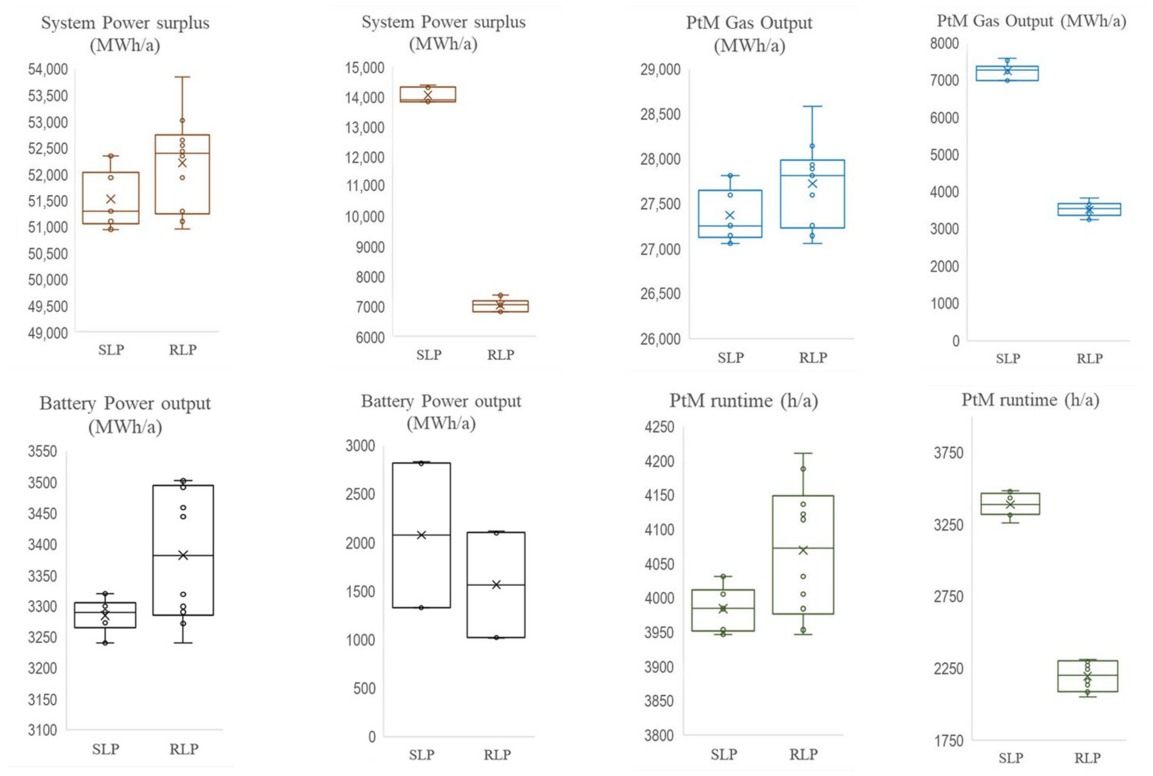
3.2. Real Load Profiles

Table A8. Simulation results for real load profiles in Straubing without PtM.

Year	Power	PV	Power	Battery	Power	Gas Grid
	Surplus	Runtime	Output	Runtime	Output	Output
SLP	[MWh/a]	[h]	[MWh/a]	[h]	[MWh/a]	[MWh/a]
2015	63,395	4390	56,625	3007	3621	597,721
2016	61,720	4367	53,691	2985	3564	599,991
2017	62,568	4380	55,053	2962	3592	599,083
2018	62,015	4379	54,895	2935	3626	598,094
2019	62,101	4379	55,047	2938	3627	598,365

,

Table A9. Simulation results for real load profiles in Straubing without PtM stored.

Year	Power	PV	Power	Battery	Power	Gas Grid	PtM	Power	Gas	Heat
	Surplus	Runtime	Output	Runtime	Output	Output	Runtime	Input	Output	Output
SLP	[MWh/a]	[h]	[MWh/a]	[h]	[MWh/a]	[MWh/a]	[h]	[MWh/a]	[MWh/a]	[MWh/a]
2015	53,837	4390	56,625	2946	3502	545,043	4188	−53,001	28,583	16,458
2016	52,536	4367	53,691	2948	3444	548,928	4114	−51,713	27,889	16,058
2017	53,013	4380	55,053	2951	3459	546,911	4122	−52,186	28,144	16,205
2018	52,420	4379	54,895	2972	3503	546,207	4136	−51,584	27,819	16,018
2019	52,637	4379	55,047	2968	3492	546,610	4211	−51,803	27,937	16,086

,

Table A10. Simulation results for real load profiles in Straubing with PtM stored.

Year	Power	PV	Power	Battery	Power	Gas Grid	PtM	Power	Gas	Heat
	Surplus	Runtime	Output	Runtime	Output	Output	Runtime	Input	Output	Output
SLP	[MWh/a]	[h]	[MWh/a]	[h]	[MWh/a]	[MWh/a]	[h]	[MWh/a]	[MWh/a]	[MWh/a]
2015	50,707	4390	56,625	2726	3508	547,656	4132	−49,936	26,931	15,507
2016	49,456	4367	53,691	2730	3442	551,614	4054	−48,701	26,264	15,123
2017	50,035	4380	55,053	2814	3472	549,755	4080	−49,273	26,573	15,301
2018	49,467	4379	54,895	2866	3502	549,070	4070	−48,698	26,263	15,122
2019	49,650	4379	55,047	2744	3507	549,484	4142	−48,880	26,361	15,179

,

Table A11. Simulation results for real load profiles in Vilshofen without PtM.

Year	Power	PV	Power	Battery	Power	Gas Grid
	Surplus	Runtime	Output	Runtime	Output	Output
SLP	[MWh/a]	[h]	[MWh/a]	[h]	[MWh/a]	[MWh/a]
2015	8853	4381	24,628	2138	1033	246,616
2016	8528	4368	23,507	2077	1019	247,209
2017	8809	4383	24,073	2119	1027	247,086
2018	8535	4376	23,884	2066	1022	246,504
2019	8568	4380	24,087	2119	1035	246,892

,

Table A12. Simulation results for real load profiles in Vilshofen without PtM stored.

Year	Power	PV	Power	Battery	Power	Gas Grid	PtM	Power	Gas	Heat
	Surplus	Runtime	Output	Runtime	Output	Output	Runtime	Input	Output	Output
SLP	[MWh/a]	[h]	[MWh/a]	[h]	[MWh/a]	[MWh/a]	[h]	[MWh/a]	[MWh/a]	[MWh/a]
2015	7363	4381	24,628	2138	1033	238,111	2305	−7129	3845	2214
2016	6814	4368	23,507	2077	1019	239,445	2243	−6583	3550	2044
2017	7132	4383	24,073	2119	1027	238,878	2314	−6899	3721	2142
2018	6822	4376	23,884	2066	1022	238,710	2272	−6590	3554	2046
2019	7044	4380	24,087	2119	1035	238,713	2301	−6809	3672	2114

and

Table A13. Simulation results for real load profiles in Vilshofen with PtM stored.

Year	Power	PV	Power	Battery	Power	Gas Grid	PtM	Power	Gas	Heat
	Surplus	Runtime	Output	Runtime	Output	Output	Runtime	Input	Output	Output
SLP	[MWh/a]	[h]	[MWh/a]	[h]	[MWh/a]	[MWh/a]	[h]	[MWh/a]	[MWh/a]	[MWh/a]
2015	7130	4381	24,628	2193	1061	237,992	2135	−6597	3558	2049
2016	6575	4368	23,507	2174	1050	239,303	2055	−6047	3261	1878
2017	6871	4383	24,073	2180	1053	238,737	2165	−6341	3420	1969
2018	6578	4376	23,884	2156	1053	238,542	2089	−6049	3262	1878
2019	6852	4380	24,087	2194	1060	238,550	2087	−6319	3408	1962

in the Appendix B show the aggregated results of the RLP simulations of SR and VOF. The use of the RLP increased the resulting power surplus for SR (Figure 13). This also resulted in a slightly increased runtime of the conversion and storage technologies compared with the SLP. For VOF, the use of RLP led to a drastic decrease in the electricity surplus. This inevitably led to reduced conversion and storage utilization. Thus, the results must be directly related to the RLP and the particular region. RLPs used for commercial and industrial applications showed larger jumps and changes in the load curves compared to the SLPs. In contrast, RLP households showed less variation over the day. This led to a smoothing of the load curve for regions containing a large share of electricity demand from households and smaller shares of commerce and industry. Because this is the case for the rural region of VOF (Figure 6), the demand composition had a much greater influence on the potential electricity surplus than at the SR site when RLP was considered.

Regarding the conversion and storage technologies, the battery and PtM runtime increased slightly in SR with the RLP data but remained on the same order of magnitude as for the SLP data. However, in VOF, the runtime of the PtM dropped by a third in comparison. This is a major problem from an economic point of view because the investment only pays off with an adequate runtime.

As already stated before, there was a difference between SLP and RLP. Figure 14 shows this difference over the year 2019 for SR by subtracting the power RLP from the SLP in kWh. Any value above zero means that the SLP was predominant and vice versa. It can be seen that, in winter, power demand via the RLP tended to be overestimated, while in summer, underestimation tended to occur in the regions. Nevertheless, it shows that strong peaks occurred over the entire year, which were mainly in the positive range. These peaks are decisive in the power sector when it comes to the necessary power storage for peak shaving. Due to this fact, it was important not only to take a top-to-bottom view with standardized values. Through a precise site analysis with the collection of local data, a much more concrete evaluation and design of storage facilities and their capacity can be made.

4. Discussion

From the case study results, general statements can be made as to whether energy storage systems should be used in the regions under consideration and which installable capacity should be used. It was shown that the PtM and battery concepts can be combined and were not mutually exclusive. An economically viable runtime and size were demonstrated for both technologies and datasets in SR. In VOF, the SLP variant had a runtime below 4000 h for the PtM and was therefore already economically difficult to represent. The decline in the RLP data to values less than 2500 h showed that detailed data collection at a local level is essential for a precise placement study to ensure economical operation. Because hydrogen generation was omitted in the model, the runtime determined for PtM can be increased by suitable H₂ storage, further optimizing the utilization rate and the capacity to be installed.

4.1. Effects of Spatial and Temporal Choices

The weather influences on the extended system over several years were examined using different years for the solar radiation data. These differences are often described as decisive when it comes to power surpluses [55]. It was shown that these weather influences almost did not affect the PV runtime and PV output, and they may play a subordinate role regarding other factors such as the demand curves or technological efficiencies.

This means that, if the district heating supply is to be expanded with CHP technologies, electricity must be produced accordingly. Therefore, PtM can only be meaningfully depicted holistically in a larger context, considering the input and output flows.

The simplifications concern both the data input from the OSM data and the available consumption data. It is known in the scientific community that OSM data are mainly collected by amateur geographers and non-specialists, which raises doubts about the quality of the OSM data used [56] (p. 514). The larger a city, the better the quality of the data because the number of volunteer mappers increases significantly with the city size [57].

Further deviations in the consumption data occur because of the standardization of the building classification, mainly owing to missing information about building type, building characteristics, or mixed building use. The larger the selected geographic energy cell under consideration, the larger the required simplifications. Depending on how one determines the number of buildings, there may be corresponding deviations here as well. Many factors must be included to determine the number. For example, a large garage falls into the category of a single-family house and is thus charged with nonexistent energy demand. While this case would not affect the year-end consumption in the study because it was determined elsewhere, it would affect the calculated average consumption for the building category. This leads to a change in the load curve. The effects of such a change can be clarified in the RLP comparison of VOF. Therefore, appropriate measures must be taken for building classification. In this study, buildings with less than a certain roof area were assigned to a building category without a demand.

Another problem is the use of the SLP or RLP. In Valdes [20], the partly strong varying correlations between SLP and RLP were examined. SLPs come close to real consumption only if the corresponding building numbers are more than 400 [58]. Because this is not the case for all building classes (Figure 6), RLPs are a potential possibility here. However, the RLPs should also originate from these buildings and also represent a group of different buildings, e.g., schools with office buildings fall into one group. Thus, the RLP assignments are also subject to certain fluctuations in the local area. Here, a further splitting below the district level could provide even more valuable factors in the decentralized supply. If this level of detail cannot be performed because of missing measuring equipment or sensitive data, one must rely on assumptions and simplifications.

4.2. Effects of Technological Choices

Another problem is the complex technology of PtM. Calliope can only integrate PtM technology with a fixed set of parameters. However, because the efficiency strongly depends on runtime, location, electricity costs, H₂/CO₂ availability, and usability of waste heat and methane, the actual gas and heat yield from this storage technology may differ significantly from the simulation result. An improvement in the results could be achieved by a simulation combination. For this purpose, the respective local framework parameters could be determined in a first Calliope simulation, which would then be transferred to another simulation tool suitable for a PtM simulation. The resulting output would then have to be incorporated into a second Calliope simulation to determine whether the result changed significantly. For this, however, the simulation tool would also require suitable interfaces to communicate with Calliope.

The battery was assumed to be a single unit with a size of 10% of the installed PV power. In times of ever better and cheaper electricity storage systems, which are also increasingly found in private households [59], the storage size of the battery could be considered decentralized. This would circumvent the limitation of fast charging to 25% of a single battery and could increase the used charging speed in the region.

A novelty of this study is the shift of the system boundary of the consideration of PtM to the injection of gas and heat into their respective grids, as well as the interaction with other technologies that take gas from the natural-gas grid and technologies that feed into a district heating grid. In the present case, renewable methane was only used in the CHP plants or for the general gas demand in the building heating sector. However, the production of biomethane is too complex and expensive to use only for the heat sector or for re-electrification. Other areas such as the mobility or chemical sector, which also rely on C-based applications, could benefit better from this methane.

4.3. Co-Products and Other Factors

In this study, it was shown that electricity surplus potential exists in small cities and rural regions and that the required electricity surplus already exists, even in regions without wind power plants. To increase the economic attractiveness of PtM, waste heat must be integrated in a meaningful way. To achieve this, district heating networks must be expanded consistently. This expansion can be performed more easily in densely populated regions than in rural areas. In Germany, municipalities and cities can also impose a connection obligation [60]. However, higher district heating utilization reduces heat released to the atmosphere from conventional power plants and CHP technologies, and it increase the utilization rate of waste heat.

With further PV expansion, the demand for conventional power plants and CHP for electricity production in summer should decrease, and the unmet heat demand can be reduced. This would counteract excess district heating in the summer. However, the increasing periods of energy surplus with such technologies as PtM lead to RNG, which can be stored and distributed in the natural-gas grid and used for CO₂-neutral CHP production on demand in the winter. On the other hand, the need for balancing power and energy storage increases with the further expansion of RES. PtM can provide this balancing power and additionally provide valuable renewable methane for other sectors. With gas and electricity prices currently rising dramatically, the shown reducing gas withdrawals can be attractive across the board.

5. Conclusions

In this study, it was shown that the holistic evaluation of surplus power conversion from renewable sources through PtM makes a high overall usage of decentralized available renewable energies possible. Two different regions for potential energy surplus were examined to operate the storage technologies. The three major energy sectors (power, heat, and gas), which are important for the energy transition, were coupled with a PtM and a battery unit. The coupling could provide valuable information regarding the electricity surplus and storage capacity needed for this surplus, which occurs in the context of gas-fired CHP and renewable energy generation in a wind-poor part of Germany, and how this can support the heating sector in the energy transition. This shows that PtM could help to increase the efficient use of renewable energy in energy cells, especially to meet heat and power demands.

PtM technology can make a major contribution to the energy transition because the issue of sector coupling is becoming increasingly important in terms of CO₂ savings as well as efficient energy usage. The technical feasibility and practicability have been proven several times. Although the legal regulations and the profitability issue are the biggest obstacles to the implementation of the technology [61], there is also a shortage of potential analyses, in the large context, where PtM can be sensibly placed and applied and from which the required input comes. Therefore, in different projects, the regional framework conditions are analyzed to determine the best sites for PtM while using different hydrogen sources, such as hydrogen from the thermochemical conversion of biological residuals [62]. There have also been efforts to increase this to a global scale [63].

Furthermore, the solar influence over several years on energy generation and storage technologies was investigated. The underlying consumption data and time series were critically reviewed, and their influence on the results was presented. The simulation program Calliope was found to be suitable for the difficult optimization of sector coupling. Further work could focus on appropriate simulation combinations to integrate the topic of PtM into Calliope with higher quality. Further investigations are needed to assess the holistic contribution of PtM in climate-friendly energy systems, including the CO₂ balance of emissions.

References

1. Hornberg, C.; Niekisch, M.; Calliess, C.; Kemfert, C.; Lucht, W.; Messari-Becker, L.; Rotter, V.S. Using the CO2 Budget to Meet the Paris Climate Targets; SRU: Berlin, Germany, 2020; Available online: https://www.umweltrat.de/SharedDocs/Downloads/EN/01_Environmental_Reports/2020_08_environmental_report_chapter_02.pdf?__blob=publicationFile&v=5 (accessed on 23 June 2021).
2. Bundesregierung. Klimaschutzgesetz: Klimaneutralität bis 2045, Bundesregierung. 2021. Available online: https://www.bundesregierung.de/breg-de/themen/klimaschutz/klimaschutzgesetz-2021-1913672 (accessed on 23 June 2021).
3. DVGW. Zwei-Energieträger-Welt; Deutscher Verein des Gas und Wasserfaches e.V.: Bonn, Germany, 2019; p. 7. [Google Scholar]
4. Thema, M.; Bauer, F.; Sterner, M. Power-to-Gas: Electrolysis and methanation status review. Renew. Sustain. Energy Rev. 2019, 112, 775–787. [Google Scholar] [CrossRef]
5. Götz, M.; Lefebvre, J.; Mörs, F.; McDaniel Koch, A.; Graf, F.; Bajohr, S.; Reimert, R.; Kolb, T. Renewable Power-to-Gas: A technological and economic review. Renew. Energy 2016, 85, 1371–1390. [Google Scholar] [CrossRef] [Green Version]
6. Graf, F.; Krajete, A.; Schmack, U. Abschlussbericht: Techno-Ökonomische Studie zur Biologischen Methanisierung bei Power-to-Gas-Konzepten; Engler-Bunte-Institut des Karlsruher Instituts für Technolgie KIT: Karlsruhe, Germany, 2014. [Google Scholar]
7. Morgenthaler, S.; Ball, C.; Koj, J.C.; Kuckshinrichs, W.; Witthaut, D. Site-dependent levelized cost assessment for fully renewable Power-to-Methane systems. Energy Convers. Manag. 2020, 223, 113150. [Google Scholar] [CrossRef]
8. Thema, M.; Weidlich, T.; Hörl, M.; Bellack, A.; Mörs, F.; Hackl, F.; Kohlmayer, M.; Gleich, J.; Stabenau, C.; Trabold, T.; et al. Biological CO2-Methanation: An Approach to Standardization. Energies 2019, 12, 1670. [Google Scholar] [CrossRef] [Green Version]
9. Reihani, E.; Motalleb, M.; Ghorbani, R.; Saoud, L.S. Load peak shaving and power smoothing of a distribution grid with high renewable energy penetration. Renew. Energy 2016, 86, 1372–1379. [Google Scholar] [CrossRef] [Green Version]
10. Shen, J.; Jiang, C.; Liu, Y.; Qian, J. A Microgrid Energy Management System with Demand Response for Providing Grid Peak Shaving. Electr. Power Components Syst. 2016, 44, 843–852. [Google Scholar] [CrossRef]
11. Kotilainen, K. Energy prosumers’ role in the sustainable energy system. In Affordable and Clean Energy; Leal Filho, W., Azul, A.M., Brandli, L., Özuyar, P.G., Wall, T., Eds.; Springer International Publishing: Cham, Switzerland, 2020; pp. 1–14. [Google Scholar] [CrossRef]
12. Heendeniya, C.B.; Sumper, A.; Eicker, U. The multi-energy system co-planning of nearly zero-energy districts—Status-quo and future research potential. Appl. Energy 2020, 267, 114953. [Google Scholar] [CrossRef]
13. Bundesnetzagentur. Bericht über die Mindesterzeugung 2019; Bundesnetzagentur für Elektrizität, Gas, Telekommunikation, Post und Eisenbahnen: Bonn, Germany, 2019; Available online: https://www.bundesnetzagentur.de/SharedDocs/Downloads/DE/Sachgebiete/Energie/Unternehmen_Institutionen/Versorgungssicherheit/Erzeugungskapazitaeten/Mindesterzeugung/BerichtMindesterzeugung_2019.pdf?__blob=publicationFile&v=3 (accessed on 23 June 2021).
14. Kriechbaum, L.; Scheiber, G.; Kienberger, T. Grid-based multi-energy systems—Modelling, assessment, open source modelling frameworks and challenges. Energy Sustain. Soc. 2018, 8, 35. [Google Scholar] [CrossRef] [Green Version]
15. Alhamwi, A.; Medjroubi, W.; Vogt, T.; Agert, C. Development of a GIS-based platform for the allocation and optimisation of distributed storage in urban energy systems. Appl. Energy 2019, 251, 113360. [Google Scholar] [CrossRef]
16. Benz, T.; Dickert, J.; Erbert, M.; Erdmann, N. Der Zellulare Ansatz. Grundlage Einer Erfolgreichen, Regionenübergreifenden Energiewende; VDE Verband der Elektrotechnik Elektronik Informationstechnik e.V.: Frankfurt, Germany, 2015; Available online: https://docplayer.org/17827249-Der-zellulare-ansatz-grundlage-einer-erfolgreichen-regionenuebergreifenden-energiewende.html (accessed on 28 June 2021).
17. Alhamwi, A.; Medjroubi, W.; Vogt, T.; Agert, C. FlexiGIS: An open source GIS-based platform for the optimisation of flexibility options in urban energy systems. Energy Procedia 2018, 152, 941–946. [Google Scholar] [CrossRef]
18. Tröndle, T.; Lilliestam, J.; Marelli, S.; Pfenninger, S. Trade-Offs between Geographic scale, Cost, and Infrastructure Requirements for Fully Renewable Electricity in Europe. Joule 2020. Available online: https://github.com/calliope-project/euro-calliope/commit/e3a2f8c1edc84ccfede8e6fd8eef1b782476fd35 (accessed on 31 July 2020).
19. Hilbers, A.P.; Brayshaw, D.J.; Gandy, A. Importance subsampling for power system planning under multi-year demand and weather uncertainty. In Proceedings of the 2020 International Conference on Probabilistic Methods Applied to Power Systems (PMAPS), Liege, Belgium, 18–21 August 2020; pp. 1–6. [Google Scholar] [CrossRef]
20. Valdes, J.; Wöllmann, S.; Weber, A.; Klaus, G.; Sigl, C.; Prem, M.; Bauer, R.; Zink, R. A framework for regional smart energy planning using volunteered geographic information. Adv. Geosci. 2020, 54, 179–193. [Google Scholar] [CrossRef]
21. Pfenninger, S. Dealing with multiple decades of hourly wind and PV time series in energy models: A comparison of methods to reduce time resolution and the planning implications of inter-annual variability. Appl. Energy 2017, 197, 1–13. [Google Scholar] [CrossRef]
22. Meier, H.; Fünfgeld, C.; Adam, T.; Schieferdecker, B. Repraesentative VDEW Lastprofile; BTU: Frankfurt, Germany, 1999. [Google Scholar]
23. Valdes, J.; Macia, Y.M.; Dorner, W.; Camargo, L.R. Unsupervised grouping of industrial electricity demand profiles: Synthetic profiles for demand-side management applications. Energy 2020, 215, 118962. [Google Scholar] [CrossRef]
24. Bundesministerium für Wirtschaft und Energie, Aktuelle Informationen: Erneuerbare Energien im Jahr 2020. Available online: https://www.erneuerbare-energien.de/EE/Navigation/DE/Service/Erneuerbare_Energien_in_Zahlen/Aktuelle-Informationen/aktuelle-informationen.html (accessed on 23 June 2021).
25. Kurmann, F. Elektrolyse als Wärmequelle. VDI Nachrichten 2021, 75, 22. [Google Scholar] [CrossRef]
26. Weiler, V.; Stave, J.; Eicker, U. Renewable Energy Generation Scenarios Using 3D Urban Modeling Tools—Methodology for Heat Pump and Co-Generation Systems with Case Study Application. Energies 2019, 12, 403. [Google Scholar] [CrossRef] [Green Version]
27. Bayerische Staatsregierung. Karten und Daten zur Energiewende; Energie-Atlas: Bayern, Germany, 2020; Available online: https://geoportal.bayern.de/energieatlas-karten/?wicket-crypt=ov0weLCjotU (accessed on 30 July 2020).
28. Pfenninger, S.; Keirstead, J. Renewables, nuclear, or fossil fuels? Scenarios for Great Britain’s power system considering costs, emissions and energy security. Appl. Energy 2015, 152, 83–93. [Google Scholar] [CrossRef] [Green Version]
29. Díaz, P.; Patt, A.; Van Vliet, O. Do We Need Gas as a Bridging Fuel? A Case Study of the Electricity System of Switzerland. Energies 2017, 10, 861. [Google Scholar] [CrossRef] [Green Version]
30. Pfenninger, S.; Pickering, B. Calliope: A multi-scale energy systems modelling framework. J. Open Source Softw. 2018, 3, 825. [Google Scholar] [CrossRef] [Green Version]
31. Luz, G.P.; Silva, R.A.E. Modeling Energy Communities with Collective Photovoltaic Self-Consumption: Synergies between a Small City and a Winery in Portugal. Energies 2021, 14, 323. [Google Scholar] [CrossRef]
32. BDEW, VKU, and GEODE. Abwicklung von Standardlastprofilen Gas; BDEW, VKU, GEODE: Berlin, Germany, 2021; Available online: https://www.bdew.de/media/documents/20210331_LF_SLP_Gas_KoV_XII_WahrfRi.pdf (accessed on 23 June 2021).
33. BDEW. Standardlastprofile Strom. Available online: https://www.bdew.de/energie/standardlastprofile-strom/ (accessed on 27 June 2021).
34. Parra, D.; Zhang, X.; Bauer, C.; Patel, M.K. An integrated techno-economic and life cycle environmental assessment of power-to-gas systems. Appl. Energy 2017, 193, 440–454. [Google Scholar] [CrossRef]
35. Schiebahn, S.; Grube, T.; Robinius, M.; Tietze, V.; Kumar, B.; Stolten, D. Power to gas: Technological overview, systems analysis and economic assessment for a case study in Germany. Int. J. Hydrogen Energy 2015, 40, 4285–4294. [Google Scholar] [CrossRef]
36. Laha, P.; Chakraborty, B. Cost optimal combinations of storage technologies for maximizing renewable integration in Indian power system by 2040: Multi-region approach. Renew. Energy 2021, 179, 233–247. [Google Scholar] [CrossRef]
37. Calliope: A Multi-Scale Energy Systems Modeling Framework. Available online: https://calliope.readthedocs.io/en/v0.6.6-post1/index.html (accessed on 16 June 2021).
38. Staffell, I.; Pfenninger, S. Using bias-corrected reanalysis to simulate current and future wind power output. Energy 2016, 114, 1224–1239. [Google Scholar] [CrossRef] [Green Version]
39. Pfenninger, S.; Staffell, I. Long-term patterns of European PV output using 30 years of validated hourly reanalysis and satellite data. Energy 2016, 114, 1251–1265. [Google Scholar] [CrossRef] [Green Version]
40. Padgham, M.; Rudis, B.; Lovelace, R.; Salmon, M. Osmdata: Import “OpenStreetMap” Data as Simple Features or Spatial Objects. 2020. Available online: https://CRAN.R-project.org/package=osmdata (accessed on 2 March 2020).
41. Bundesnetzagentur. Veröffentlichung von EEG-Registerdaten. Available online: https://www.bundesnetzagentur.de/DE/Sachgebiete/ElektrizitaetundGas/Unternehmen_Institutionen/ErneuerbareEnergien/ZahlenDatenInformationen/EEG_Registerdaten/EEG_Registerdaten_node.html (accessed on 5 July 2020).
42. C.A.R.M.E.N. e.V. Marktübersicht Batteriespeicher 2020, Centrales Agrar-Rohstoff Marketing- und Energie-Netzwerk, Straubing, Erneuerbare Energien 1. 2020. Available online: https://www.carmen-ev.de/files/Sonne_Wind_und_Co/Speicher/Marktuebersicht-Batteriespeicher_2020.pdf (accessed on 1 June 2020).
43. PEM Electrolysers and Stacks: H-TEC SYSTEMS Products. Available online: https://www.h-tec.com/en/products/ (accessed on 20 March 2022).
44. Friedl, D.M.; Meier, B.; Ruoss, F.; Schmidlin, L. Thermodynamik von power-to-gas. In Hochschule für Technik, Rapperswil; Institut für Energietechnik: Amberg, Germany, 2017; p. 67. [Google Scholar]
45. Alhamwi, A.; Medjroubi, W.; Vogt, T.; Agert, C. Modelling urban energy requirements using open source data and models. Appl. Energy 2018, 231, 1100–1108. [Google Scholar] [CrossRef]
46. Alhamwi, A.; Medjroubi, W.; Vogt, T.; Agert, C. OpenStreetMap data in modelling the urban energy infrastructure: A first assessment and analysis. Energy Procedia 2017, 142, 1968–1976. [Google Scholar] [CrossRef]
47. Schellong, W. Analyse und Optimierung von Energieverbundsystemen; Springer: Berlin/Heidelberg, Germany, 2016. [Google Scholar] [CrossRef]
48. Schröder, R.N.F.; Altendorf, L.; Greller, M.; Boegelein, T. Universelle Energiekennzahlen für Deutschland: Teil 4: Spezifischer Heizenergieverbrauch kleiner Wohnhäuser und Verbrauchs—Hochrechnung für den Gesamtwohnungsbestand. Bauphysik 2011, 33, 243–253. [Google Scholar] [CrossRef]
49. BDEW, VKU, and GEODE. Evaluierungsbericht der Verteilernetzbetreiber zu der Prognosegüte der Standardlastprofile Gas; BDEW, VKU, GEODE: Berlin, Germany, 2021; Available online: https://www.bdew.de/media/documents/2021-03-31_SLP-Evaluierungsbericht.pdf (accessed on 23 June 2021).
50. Ruhnau, O.; Hirth, L.; Praktiknjo, A. Time series of heat demand and heat pump efficiency for energy system modeling. Sci. Data 2019, 6, 189. [Google Scholar] [CrossRef]
51. Schüler, N.; Mastrucci, A.; Bertrand, A.; Page, J.; Marechal, F. Heat Demand Estimation for Different Building Types at Regional Scale Considering Building Parameters and Urban Topography. Energy Procedia 2015, 78, 3403–3409. [Google Scholar] [CrossRef] [Green Version]
52. Bundesministerium für Wirtschaft und Energie. So Heizen die Deutschen. 2019. Available online: https://www.bmwi-energiewende.de/EWD/Redaktion/Newsletter/2019/10/Meldung/direkt-erfasst_infografik.html (accessed on 23 June 2021).
53. BDEW. Energiemarkt Deutschland 2020; Wirtschafts und Verlagsgesellschaft Gas und Wasser mbH: Bonn, Germany, 2020; p. 52. [Google Scholar]
54. Bundesamt für Justiz, § 8 EEG 2021—Einzelnorm. 2014, p. 154. Available online: https://www.gesetze-im-internet.de/eeg_2014/__8.html (accessed on 17 June 2021).
55. Camargo, L.R.; Valdes, J.; Macia, Y.M.; Dorner, W. Assessment of on-site steady electricity generation from hybrid renewable energy systems in Chile. Appl. Energy 2019, 250, 1548–1558. [Google Scholar] [CrossRef]
56. Mooney, P.; Corcoran, P.; Winstanley, A.C. Towards quality metrics for OpenStreetMap. In Proceedings of the 18th SIGSPATIAL International Conference on Advances in Geographic Information Systems—GIS ’10, San Jose, CA, USA, 2–5 November 2010; p. 514. [Google Scholar] [CrossRef] [Green Version]
57. Pach, D. Seminar: MobileGIS OpenStreetMap Datenqualität und Quantiät. Uni Augsburg. 2012. Available online: https://www.informatik.uni-augsburg.de/lehrstuehle/dbis/db/lectures/ss11/mobileGIS/themen/Thema12_Ausarbeitung_Pach.pdf (accessed on 25 August 2020).
58. Von Appen, J.; Haack, J.; Braun, M. Erzeugung zeitlich hochaufgelöster Stromlastprofile für Verschiedene Haushaltstypen, Presented at the IEEE Power and Energy Student Summit (PESS). 2014. Available online: https://www.researchgate.net/publication/273775902_Erzeugung_zeitlich_hochaufgeloster_Stromlastprofile_fur_verschiedene_Haushaltstypen (accessed on 28 June 2021).
59. Figgener, J.; Stenzel, P.; Kairies, K.-P.; Linßen, J.; Haberschusz, D.; Wessels, O.; Angenendt, G.; Robinius, M.; Stolten, D.; Sauer, D.U. The development of stationary battery storage systems in Germany—A market review. J. Energy Storage 2020, 29, 101153. [Google Scholar] [CrossRef]
60. Bundesamt für Justiz, § 109 GEG—Einzelnorm. 2020, p. 87. Available online: https://www.gesetze-im-internet.de/geg/__109.html (accessed on 23 June 2021).
61. Bründlinger, T.; König, J.; Frank, O.; Gründig, D.; Jugel, C.; Kraft, P. Integrierte Energiewende, Dena Deutsche Energie-Agentur GmbH, Berlin, Leitstudie. 2018. Available online: https://www.dena.de/themen-projekte/projekte/energiesysteme/dena-leitstudie-integrierte-energiewende/ (accessed on 23 June 2021).
62. DANUP-2-GAS. Interreg Danube. 2020. Available online: http://www.interreg-danube.eu/approved-projects/danup-2-gas (accessed on 28 June 2021).
63. Pfennig, M.; Bonin, M.; Gerhardt, N. Ptx-Atlas: Weltweite Potenziale für Die Erzeugung von Grünem Wasserstoff und Klimaneutralen Synthetischen Kraft—Und Brennstoffen; Fraunhofer IEEE Institute für Energiewirtschaft und Energietechnik: Kassel, Germany, 2021; Available online: https://www.iee.fraunhofer.de/content/dam/iee/energiesystemtechnik/de/Dokumente/Veroeffentlichungen/FraunhoferIEE-PtX-Atlas_Hintergrundpapier_final.pdf (accessed on 28 June 2021).
Figure 1. Structure of the simplified model with data sources.
Energies 15 02640 g001
Figure 2. Abstract concept for a Power-to-Methane (PtM) unit implemented in Calliope from Valdes et al. [20].
Energies 15 02640 g002
Figure 3. Map of Straubing.
Energies 15 02640 g003
Figure 4. Map of Vilshofen at the Danube.
Energies 15 02640 g004
Figure 5. Aggregated demand for different energy carriers in MWh/a.
Energies 15 02640 g005
Figure 6. Demand share by region and building category ((a) Straubing and (b) Vilshofen): H1 (single family house), H2 (multiple family house), G1 (business weekdays), G2 (business evening), G3 (business 24/7), G4 (trade), G5 (bakery), G6 (business weekend), and BI (industry).
Energies 15 02640 g006
Figure 7. Share of building category by region ((a) Straubing and (b) Vilshofen): H1 (single family house), H2 (multiple family house), G1 (business weekdays), G2 (business evening), G3 (business 24/7), G4 (trade), G5 (bakery), G6 (business weekend), and BI (industry).
Energies 15 02640 g007
Figure 8. Power demand line of Straubing in February with RLP.
Energies 15 02640 g008
Figure 9. Power demand line of Straubing in February with SLP.
Energies 15 02640 g009
Figure 10. Heat demand line of Straubing in February with RLP.
Energies 15 02640 g010
Figure 11. Heat demand line of Straubing in February with SLP.
Energies 15 02640 g011
Figure 12. Simulation results comparing the PtM scenarios for SR.
Energies 15 02640 g012
Figure 13. Simulation results for PtM, for SLP, and for RLP in SR and VOF.
Energies 15 02640 g013
Figure 14. Mean deviation between SLP and RLP power for SR during 2019.
Energies 15 02640 g014