Article

Stochastic Generation Scheduling of Insular Grids with High Penetration of Photovoltaic and Battery Energy Storage Systems: South Andaman Island Case Study

1
Department of Electrical Engineering, School of Technology, Pandit Deendayal Energy University, Gandhinagar 382010, Gujarat, India
2
MCAST Energy Research Group, Institute of Engineering and Transport, Malta College of Arts, Science and Technology (MCAST), Corradino Hill, PLA 1260 Paola, Malta
3
Department of Mathematics, School of Technology, Pandit Deendayal Energy University, Gandhinagar 382010, Gujarat, India
*
Author to whom correspondence should be addressed.
Energies 2022, 15(7), 2612; https://doi.org/10.3390/en15072612
Submission received: 7 February 2022 / Revised: 14 March 2022 / Accepted: 21 March 2022 / Published: 3 April 2022
(This article belongs to the Special Issue Future Integration of Photovoltaic Systems)

Abstract

:
Insular grids are fragile owing to lower inertia and the absence of interconnection with other grids. With the increasing penetration of non-dispatchable renewable energy sources, the vulnerability of such insular grids increases further. The government of India has proposed several projects to improve the photovoltaic systems (PV) penetration in the Andaman and Nicobar Islands’ grid. This paper investigates joint stochastic scheduling of energy and reserve generation for insular grids fed from diesel and gas-based generators, PV, and battery energy storage systems (BESS). The proposed stochastic scheduling model considers a wide range of probabilistic forecast scenarios instead of a deterministic model that assumes a single-point forecast. Hence, it provides an optimal solution that is technically feasible for a wide range of PV power forecast scenarios. The striking feature of the model developed in this work is the inclusion of stochastic constraints that represent (i) the coordination between PV and BESS, (ii) reserve constraints, (iii) battery charging/discharging limit constraints, and (iv) non-anticipatory constraints that ensure technical viability of scheduling decisions. The proposed model is validated on the dataset for South Andaman Island. Results reveal the applicability and feasibility of the proposed stochastic dispatch model for different generation mix scenarios.

1. Introduction

Non-interconnected insular grids of Andaman and Nicobar (A&N) Islands predominantly supply electricity through diesel generator power houses (DGPH). Since the fuel cost of DGPH is high, the cost of electricity produced in the A&N Islands is higher than in the mainland. Moreover, many of these DGPH have generators with low efficiency and high emission levels of greenhouse gases (GHG). Over-dependency on fossil fuels and transportation of these fuels through ships also poses a significant challenge for insular grids of the A&N archipelago [1,2]. Similar circumstances are observed in several insular grids around the globe, which has given impetus to the proliferation of Renewable Energy Sources (RES) [3,4,5]. The government of India has initiated several projects to increase the penetration of PV power in the conventional grid of A&N islands [6]. Therefore, it has become necessary for insular grids, such as that of A&N islands, to plan generation dispatch schedules capable of handling the uncertainties associated with RES while also ensuring that the dispatch is economical [7].
The generation scheduling problem is essential for the smooth operation of an insular grid. Its objective is to minimize the total fuel cost of the electrical power-generated subject to the technical satisfaction of individual unit constraints and overall system constraints. System operators ensure that conventional generators’ commitment and scheduling levels are decided well in advance of the actual delivery of power to deal with different system uncertainties. In the past, the only uncertainties considered were the forecasting error of predicted load and the non-availability of system components, such as generators, transformers, transmission lines, etc. However, with increasing penetration of RES, such as wind and solar, system operators have to consider the stochasticity associated with the intermittent nature of RES and other uncertainties before deciding generation dispatch levels of conventional generators [8]. The grid structure of islands is fragile and vulnerable to stability issues owing to lower system inertia and the absence of interconnection with the neighboring grids. Hence, integration of intermittent RES with insular grids can raise critical operational challenges for generation scheduling [9].
Researchers have addressed the RES intermittency issue in two ways: either by enhancing the forecast qualities through different prediction models [10] or by optimal management of the generation scheduling problem in such a manner that the impact of variable output from RES is accommodated [11]. The latter approach is achieved by appropriate mathematical formulations that incorporate the constraints that can deal with volatility associated with RES. Generally, power output from RES varies from the actual commitment made in the day-ahead market. In such a scenario, the system operators have to provide sufficient reserves to accommodate the power output variability of RES. In mainland grid systems, reserves are provided by synchronous machines of conventional energy sources. However, in insular grids, reserves are provided by traditional sources and energy storage systems, such as pumped hydro storage systems and battery storage [12,13,14]. A generation scheduling model is investigated in [15] for insular grids with a high share of wind turbines and photovoltaic systems (PV). The two variants of the scheduling model presented in [15] are (i) through a detailed commitment model with temporal reserve constraints that include primary, secondary, and tertiary constraints within its deterministic formulation and (ii) through a more practical and simplistic model that builds schedules based on aggregate spinning reserves. However, these models have considered reserve capacities from conventional generators alone. They have not considered the impact on the structure of mathematical formulation if energy storage systems are to be included as a part of the reserve capacity. Reference [16] proposed an optimization model for isolated systems with battery energy storage systems (BESS). This model, however, does not discuss the interplay between RES and BESS. A hybrid power station consisting of wind turbines, pumped hydro storage and BESS facilities are reported in [17]. The focus is on the coordinated operation of RES and energy storage technologies in their proposed mathematical formulation. The objective function of the proposed model in reference [17] is to maximize the profit earned from the hybrid power station since the model is from the station owner’s perspective and not from the system operator’s (SO). References [18,19,20] reported deterministic generation dispatch models wherein its power-output-point forecast represents RES. Hence, the optimal commitment and generation scheduling levels have not considered the uncertain characterization of a probabilistic forecast. Intermittency and volatility associated with RES influence the optimality and technical feasibility of the generation schedule. Thus, considering a probabilistic forecast within the mathematical formulation of a dispatch model is better than considering a deterministic forecast. Stochastic models incorporate the uncertainty characterization of the RES within the framework of the optimization problem.
The stochastic generation dispatch model proposed in [21] primarily focuses on the requirement of reserves in an insular grid with high wind penetration. It mainly discusses a two-stage stochastic model formulation focusing on quantifying spinning and non-spinning load following reserves. However, although wind spillage variables have been included in the formulation, there is no discussion on how storage facilities can minimize wind spillage. Authors of work [22] proposed a generation scheduling model for insular grids with RES and pumped storage facilities. The stochastic variable considered is the availability/non-availability of thermal plants, modeled using Monte Carlo simulation, whereas RES is represented by its point forecast [22]. A two-stage stochastic model proposed in [23] considers wind as a stochastic variable and includes the coordination between RES and storage technology within the mathematical formulation. But since wind and pumped hydro storage facilities, the mathematical formulation is structured around the technical needs of pumped storage technologies. A summary of the literature survey for reference work [15,16,17,18,19,20,21,22,23,24] is shown in Table 1. Comparison of different optimal scheduling strategies shown in Table 1 suggests that a stochastic formulation with technical constraints supporting the inclusion of PV and BESS in insular grids has not been discussed to date to the best of our knowledge. Moreover, mathematical formulation representing coordination of PV with BESS has also not been investigated yet.
This work fills this lacuna by proposing a stochastic framework of a generation dispatch model that includes scheduling conventional generation, such as diesel generators (DG) and LNG-based power plants in a grid with high penetration of PV and BESS. The main contributions of this work are: (i) stochastic constraints that model the coordination of PV and BESS; (ii) stochastic reserve constraints that include the reserve contribution of conventional generators and BESS; (iii) stochastic constraints that model BESS’s charging/discharging limits; and (iv) non-anticipatory constraints that ensure technical feasibility of scheduling decisions after including variables associated with PV and BESS. Detailed investigation of the South Andaman Island for different generation portfolio mixes include DG- and LNG-based gas power plants, PV, and BESS, thereby validating the proposed model’s implementation. The paper is organized as follows: The introduction in Section 1 is followed by the mathematical formulation of the proposed model in Section 2, which comprises the theoretical background of the stochastic formulation, model description, and a detailed discussion on the proposed stochastic constraints. In Section 3, the results of the various simulation-based analysis are presented and discussed. Section 4 summarizes and concludes the overall study contributions.

2. Mathematical Formulation

This work proposes a two-stage stochastic model using the recourse approach for the generation scheduling problem of insular grid systems. The energy and reserve markets are scheduled simultaneously. The conventional energy sources considered in this work are DG and the future potential of gas-based power plants, while the non-conventional sources consist of PV with BESS. It is assumed that power provided by DG-/LNG-based power plants is bid at the marginal price of the generator. With this backdrop, the theoretical background of the two-stage recourse approach adopted in the proposed model is discussed in Section 2.1. The general mathematical framework of the proposed model is described in Section 2.2, followed by a detailed discussion on the proposed stochastic constraints in Section 2.3.

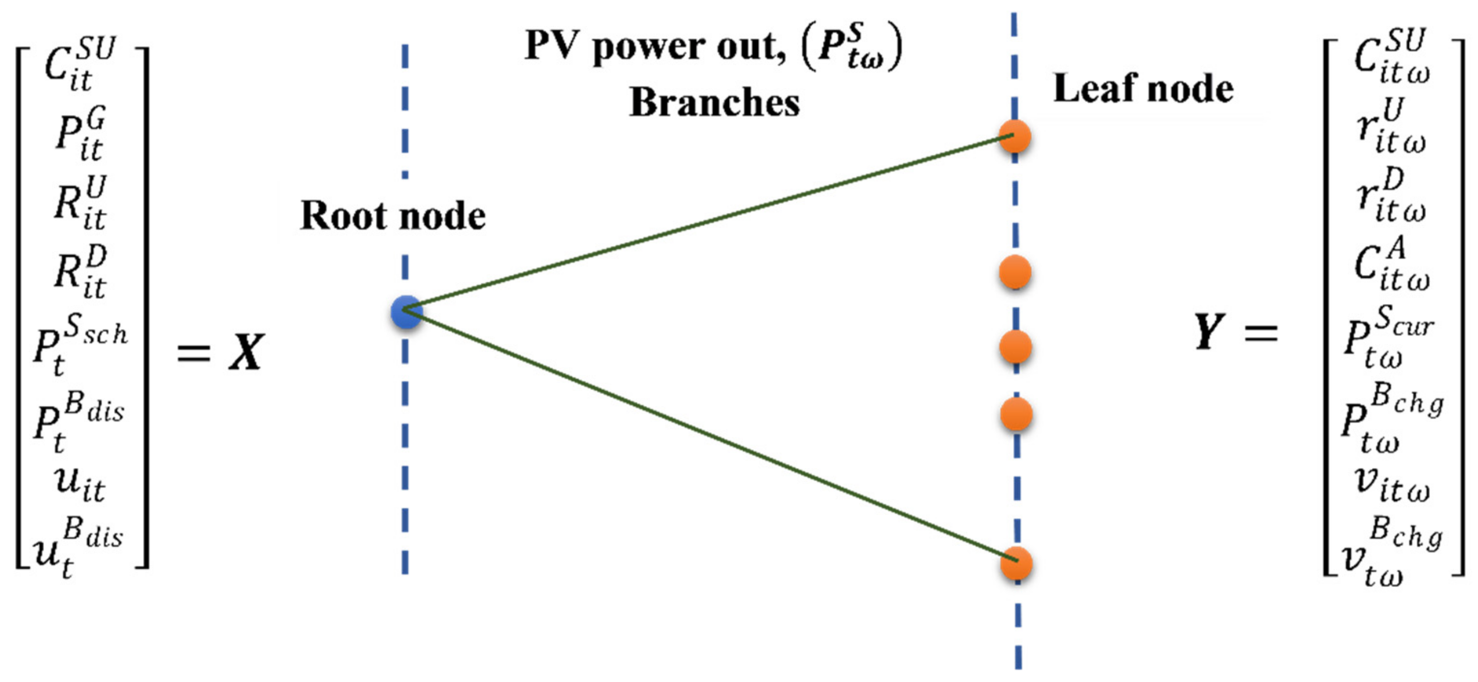
2.1. Theoretical Background of the Approach Adopted by the Proposed Stochastic Model

The fundamental elements of a recourse approach are the stochastic processes and the different decision-making stages. In a two-stage formulation of recourse approach, the first stage decisions are referred to as here-and-now decisions, while the second stage decisions are referred to as wait-and-see decisions. Decision vector X , associated with the here-and-now decisions, pertains to decisions taken before the actual realization of the stochastic process. For all practical purposes, these are the decisions that are actually implemented in the day-ahead market. All the scheduling decisions, such as the generation schedule of the DG, PV farms, and BESS, and the reserve planning decisions, such as up/down spinning reserve provided by the DG and the BESS, are first-stage decisions. On the other hand, the second stage decision vector, Y , pertains to those decisions taken after the realization of the stochastic process, φ . Hence, the second stage decision vector, Y , depends upon (i) the first stage decision vector, X , and (ii) the realization of the stochastic process, φ ω . In other words, Y can be expressed as Y X , ω , where ω is the individual scenario that would possibly realize with a specific probability of occurrence. A set of realizable scenarios, ω, are formed using scenario generation techniques.
In this work, the probabilistic forecast of PV is treated as the stochastic process, φ, whose value is unknown to the system operator. The second stage decision vector, Y , is associated with variables, such as reserve potential of conventional generators, curtailment of power from PV, BESS charging, etc.
The scenario tree is shown in Figure 1 pictorially explains the recourse’s two-stage decision framework described above. Here, the here-and-now decision vector, X , and wait-and-see decision vector, Y , are represented by the root node and leaf node, respectively, while the branches represent the stochastic process. The number of branches depends on the total number of individual scenarios, N ω , considered for the stochastic process.

2.2. Description of the Proposed Stochastic Model

The basic mathematical framework of the proposed joint energy and reserve generation dispatch model, based on the recourse approach, is formulated in (1) to (19). The nomenclature of modeling parameters, variables, and related acronyms used throughout the paper are presented in Table 2 and Table 3, respectively.

2.2.1. Objective Function

The objective function in (1) reflects here-and-now costs as well as wait-and-see costs. Here-and-now costs are associated with the first stage start-up cost, C i t S U ; energy cost, λ i t G P i t G ; and reserve capacity cost, ( λ i t R U R i t U + λ i t R D R i t D ). Wait-and-see costs are associated with the second stage start-up costs, C i t ω A ; reserve potential costs, λ i t G r i t ω G ; and penalty costs, C t ω p e n . The penalty term is to ensure that curtailment of PV and load not served is restricted.
min t = 1 N t i = 1 N i C i t S U + λ i t G P i t G + λ i t R U R i t U + λ i t R D R i t D + + t = 1 N t [ i = 1 N i ω = 1 N i π ω C i t ω A + λ i t G r i t ω G + C t ω p e n ]

2.2.2. Constraint Functions

The first constraint, represented in (2), refers to the load balance constraint. This constraint ensures that the power scheduled for conventional generators, P i t G ; for PV, P t S s c h ; and the power discharged by BESS, P t B d i s , is equal to point forecast of load, P t D , for all individual time interval, t . This constraint is primarily responsible for preparing the generation schedule for the next hour/day/any other time interval slots in the future.
i = 1 N i P i t G + P t S s c h + P t B d i s = P t D ;   i ,   t
Constraints represented in (3) to (8) are boundary constraints. These are associated with DG- and LNG-based power plant related variables, such as scheduled energy, P i t G ; reserve capacity, R i t U   and   R i t D ; and reserve potential, r i t ω U   and   r i t ω D . Generation limit ( P i m i n ,   P i m a x ) constraints of the conventional sources considering up- and down-reserve capacity are represented by (3) and (4).
P i m i n u i t P i t G R i t D ;   i ,   t
P i m a x u i t P i t G + R i t U ;   i ,   t
Similarly, (5) and (6) represent the maximum and minimum limits of spinning reserve capacity provided by each conventional generator.
0 R i t U R i U m a x u i t ;   i ,   t
0 R i t D R i D m a x u i t   ;     i ,   t
All the above boundary constraints are first-stage constraints. The next two boundary constraints in (7) and (8) are second-stage constraints. They give upper and lower bounds of the reserve potential technically possible for individual conventional generators.
0 r i t ω U R i U m a x u i t   ;   i ,   t ,   ω
0 r i t ω D R i D m a x u i t ;   i ,   t   ,   ω
One of the non-anticipatory constraints associated with up/down-reserve potential variables is represented by (9).
r i t ω U r i t ω D = r i t ω G ;   i ,   t ,   ω
In case of limits on the dispatch schedule of power produced by PV, P t S s c h , the lower ( F t S m i n ) and upper bounds, F t S m a x , of PV’s probabilistic forecasts is considered as the minimum and maximum boundary limits as seen in (10).
F t S m i n P t S s c h F t S m a x ;   t
Constraints in (11) to (13) are associated with start-up costs. First stage start-up constraints and second stage start-up constraints are presented in (11) and (12).
λ i S U u i t u i , t 1 C i t S U ;   i ,   t
λ i S U v i t ω v i , t 1 , ω C i t ω S U ;   i ,   t ,   ω
Since the start-up constraints are temporal constraints, commitment status at the time, t , ( u i t ,   v i t ω ), and commitment status at t 1 , u i , t 1 ,   v i , t 1 , ω , are considered in (11) and (12). A non-anticipatory constraint connects the first- and second-stage start-up variables in (13).
C i t ω S U C i t S U = C i t ω A ;   i ,   t ,   ω
Here, it is to be noted that C i t S U , C i t ω S U , and C i t ω A are start-up variables, while λ i S U is a constant parameter representing the start-up cost of a generator, i .
Overall penalty cost involving the sum of penalty due to PV’s curtailment and penalty owing to load shedding decision is represented by (14).
λ S c u r P t ω S c u r + λ D n s P t ω D n s = C t ω p e n ;   t ,   ω
The nature of all the decision variables considered in the overall problem is defined in (15) to (19). In (15), it is seen that all here-and-now variables are non-negative. A similar comment on the non-negativity of the wait-and-see variables is made in (16).
C i t S U ,   P i t G ,   R i t U ,   R i t D ,   P t S s c h ,   P t B d i s ,   u i t ,   u t B d i s 0 ;   i ,   t
C i t ω S U ,   r i t ω U ,   r i t ω D ,   P t ω S c u r , P t ω B ,   P t ω B c h g ,   v i t ω ,   v t ω B c h g 0 ; i ,   t , ω
The first- and second-stage variables, shown in (17) and (18), respectively, are continuous, while (19) represents variables that are binary integers.
C i t S U ,   P i t G ,   R i t U ,   R i t D ,   P t S s c h ,   P t B d i s R ;   i ,   t
C i t ω S U ,   r i t ω U ,   r i t ω D ,   P t ω S c u r , P t ω B ,   P t ω B c h g R ;   i ,   t , ω
u i t ,   u t B d i s ,   v i t ω ,   v t ω B c h g 0 , 1 ;   i ,   t , ω
Some variables listed in (16) to (19) are neither present in the objective function nor the constraint functions. These variables shall appear in the proposed constraints in Section 2.3.

2.3. Proposed Stochastic Constraints

An insular grid with conventional generators and PV farms has been considered in this work. Most PV power plants are designed with provisions for energy storage units. Hence, BESS is included in this work. Three different constraints are proposed to accommodate PV power plants and BESS in an insular grid’s commitment and generation scheduling model. These constraints ensure the technical viability of the schedule and maintain non-anticipativity between the first- and second-stage decision variables. These constraints are discussed at length in Section 2.3.1, Section 2.3.2 and Section 2.3.3.

2.3.1. Constraints That Represent the Coordination between PV and BESS

Consider a specific scenario, ω , wherein the PV power output realized in real-time is forecasted to be P t ω S . If this realization is more than the scheduled PV power, P t S s c h , then either conventional generation has to be reduced, or BESS has to be charged, or power from PV has to be curtailed, or a combination of all these options has to be implemented. On the other hand, if PV power output realized in real-time is less than the scheduled power, the generation of DG would have to be ramped up, or stored energy of BESS has to be discharged, or load shedding has to be implemented as a last measure. A mathematical model incorporating these conditions is shown in (20). This constraint consists of both here-and-now variables and wait-and-see variables. The term representing power from DG/LNG includes the first-stage scheduled power term, P i t G , and the second-stage reserve potential, r i t ω G , of each DG. Similarly, the net power of the battery includes the first-stage variable, scheduled power to be discharged, P t B d i s , and the second-stage variable, charging power, P t ω B c h g , which would vary with every changing scenario, ω . The power from PV is represented by the realized forecast scenarios, P t ω S , and the possible curtailment in the wait-and-see stage, P t ω S c u r . Load demand, in (20), consists of the point forecast of load demand, ( P t D ), at the time, t , and the load not served, ( P t ω D n s ), depending on the scenario, ω .
i = 1 N i P i t G + r i t ω G P o w e r   f r o m   D G + P t ω S P t ω S c u r P o w e r   f r o m   P V + P t B d i s P t ω B c h g P o w e r   f r o m   B E S S = P t D P t ω D n s L o a d   D e m a n d ;   i ,   t ,   ω
To reduce redundancy, (21) is formed by subtracting (2) from (20). The new proposed constraint (21) replaces (20) in the stochastic generation scheduling problem.
i = 1 N i r i t ω G + P t ω S P t ω S c u r P t ω B c h g + P t ω D n s P t S s c h = 0 ;     i ,   t ,   ω
An additional linking constraint is shown in (22), which ensures that the PV power realization, P t ω S , in the scenario, ω , accounts for the scheduled power from PV, P t S s c h , and the power consumed while charging the battery, P t ω B c h g . If the system constraints do not allow the full utilization of the power from PV in generation scheduling or battery charging, then the remaining power is curtailed. This is mathematically depicted in constraint (22).
P t ω S = P t S s c h + P t ω B c h g + P t ω S c u r ;   i ,   t ,   ω

2.3.2. Constraints That Represent System Reserve and Individual Reserve Capacities

Proposed modifications in system spinning reserve constraints for up- and down-reserve capacity are represented by (23) and (24). The purpose of these reserve constraints is to consider the inaccuracies associated with demand forecasts, P t D , and probabilistic power forecasts from PV, P t ω S . A certain percentage of demand forecast and PV’s power output scheduled in the day-ahead schedule, before the actual realization, is to be provided as up/down spinning reserve. This is seen in (23) and (24), wherein conventional generators provide for α % of the demand, P t D , and β % of the scheduled power from PV, P t S s c h , as up-reserve, R i t U , and down-reserve, R i t U . Other than the terms mentioned above, P t ω B , the current battery power status, is also mentioned in (23) and (24). Variable P t ω B indicates the amount of power that can be discharged by BESS when there is a need for up-reserve owing to underproduction of power output from PV or rise in load demand. The term ( P B m a x P t ω B ), in (24), indicates the amount of power that can be charged into the battery to provide down-reserve under the scenario of unexpected fall in demand or actual power realization from PV being more than committed level.
i = 1 N i R i t U + P t ω B α P t D + β P t S s c h ;     i ,   t ,   ω
i = 1 N i R i t D + P B m a x P t ω B α P t D + β P t S s c h ; i ,   t ,   ω
System reserve constraints, given by (23) and (24), cover the entire system’s up/down spinning reserve requirements. The following constraint represents the reserve potential of individual generators. Minimum and maximum generation limits of all individual generators with all reserves considered are modeled by (25) for each generator under different forecasting scenarios. Here, variable v i t ω is the stochastic commitment variable that shows the commitment status of DG-/LNG-based power plants under individual forecasting scenarios.
P i G m i n v i t ω P i t G + R i t U R i t D + r i t ω G P i G m a x v i t ω ;     i ,   t ,   ω

2.3.3. BESS Charging and Discharging Limit Constraints and Other Constraints

The last category of constraints is associated with the charging and discharging limits of BESS and other technical constraints associated with it. Battery charging status, P t ω B , is represented as shown in (26), wherein it can be seen that the current status of battery power, P t ω B , depends on the previous battery power status, P t 1 , ω B , and charging/discharging status of the battery in the current time interval, P t ω B c h g / P t B d i s . Here, η c h g and η d i s refer to the charging and discharging efficiency of BESS. Constraint (26) is an inter-temporal constraint. The upper and lower bounds of battery status are as given in (27).
P t ω B = P t 1 , ω B + η c h g P t ω B c h g P t B d i s η d i s ;     i ,   t ,   ω
0 P t ω B P B m a x ;     i ,   t ,   ω  
A battery may either charge or discharge energy. Charging and discharging of BESS do not coincide. To ensure that the mathematical solution obtained using the formulation discussed until now does not override this technical condition, two binary variables, u t B d i s and v t ω B c h g , are introduced in (28) and (29). The positioning of these variables in (28) and (29) ensure that decision on discharging and charging of BESS is not happening simultaneously in any given time interval, t .
P t ω B d i s P B m a x u t B d i s ; i ,   t ,   ω
P t ω B c h g P B m a x v t ω B c h g u t B d i s ;     i ,   t ,   ω
Power discharged from the battery at any time, t , cannot exceed the power available in the battery at that time. This constraint is depicted by (30).
P t B d i s P t 1 , ω B ; i ,   t ,   ω
All the above constraints discussed in Section 2.3.1, Section 2.3.2 and Section 2.3.3are included in the generation scheduling model described in Section 2.2 to form the proposed generation scheduling model of an insular grid with high penetration of PV and BESS.

3. Results and Discussion through the Case Study of South Andaman Island

In this section, the proposed model is validated on the system information of South Andaman Island. A short system description is given in Section 3.1, followed by the simulation results in Section 3.2.

3.1. System Description

Andaman and Nicobar (A&N) Islands is an archipelago of 572 islands in the Bay of Bengal, of which only 37 are inhabited. All of these islands are insular grids with independent electrical networks. They are neither connected to the mainland, nor are they interconnected. The southernmost island, South Andaman Island, has the highest load demand [25,26]. The power system of South Andaman consists of different diesel generator power houses (DGPH) distributed on a 33 kV transmission network. Due to high fuel costs, the cost of electricity generated by DGPH is expensive. DGPH is also responsible for high levels of GHG emissions. Therefore, the government of India is investigating several project proposals on increasing PV penetration in South Andaman Island. In addition to the existing 5 MWp PV farm and 1 MWp of rooftop PV, in June 2020, a 20 MWp PV farm with an 8 MWh BESS was commissioned in South Andaman Island [19]. There are discussions for further increasing the installed capacity of PV farm to 50 MWp with BESS of 20 MWh capacity.
The installed capacity of the existing DGs is as shown in Table 4. Here, Chatham power house (CPH), Phoenix Bay power house (PBPH), and hiring power plants (HPPs) represent the existing DGPHs. HPPs are diesel generator (DG) sets provided by private entities that have entered into a contractual agreement with the electricity department (A&N administration) for supplying power during peak periods. Some of these HPPs have several similar small-sized DGs, such as HPP3, which has seven DGs of 1.0 MVA each. In Table 4, for convenience, some of these generators are clubbed together. For instance, HPP3 is represented by one generator of 2 MW and the other of 5 MW. Other details mentioned in Table 4, such as minimum and maximum generation limits and up- and down-reserve limits, are scaled-down versions of the generator data provided in [10]. In contrast, the generation costs, reserve costs, and start-up costs are values based on the general pricing trend prevalent in South Andaman Island but not necessarily the costs of the individual DGPH.

3.2. Simulation Results

There are two distinguishing characteristics of the PV and load profile of A&N Islands.
(i)
Its weather characteristics are similar to the tropical belt, where sunshine is available until around 03:00 p.m., followed by tropical rains. Hence, PV’s power is available only till late afternoons.
(ii)
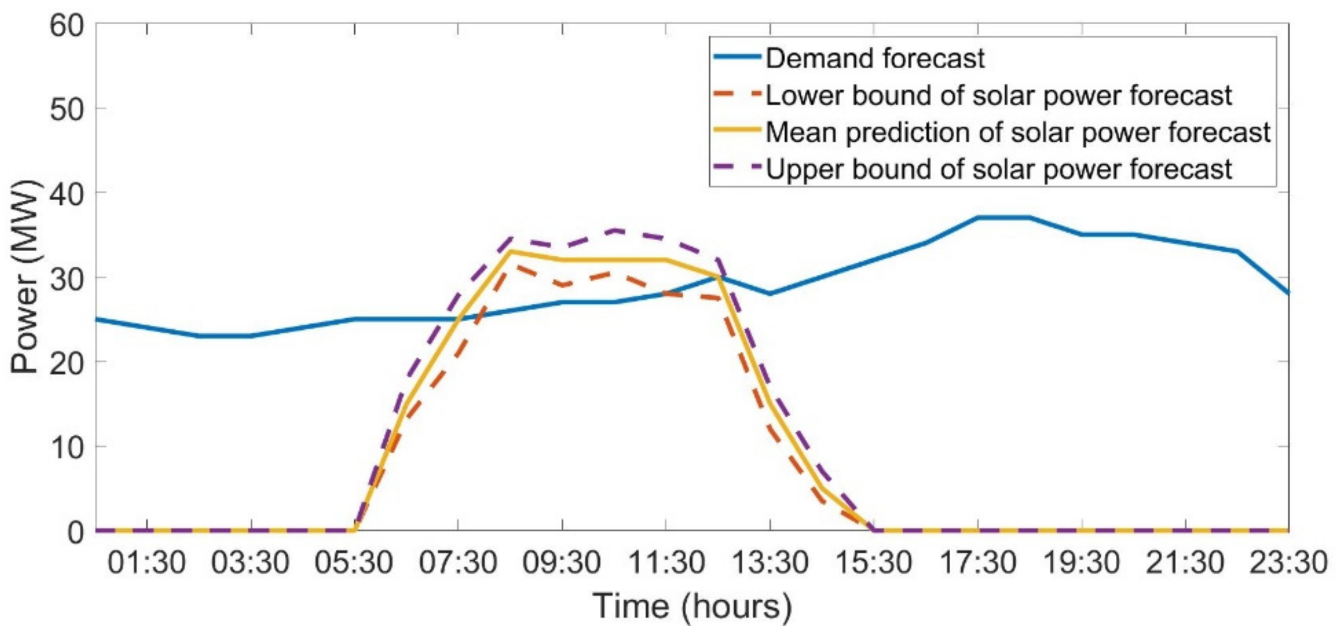
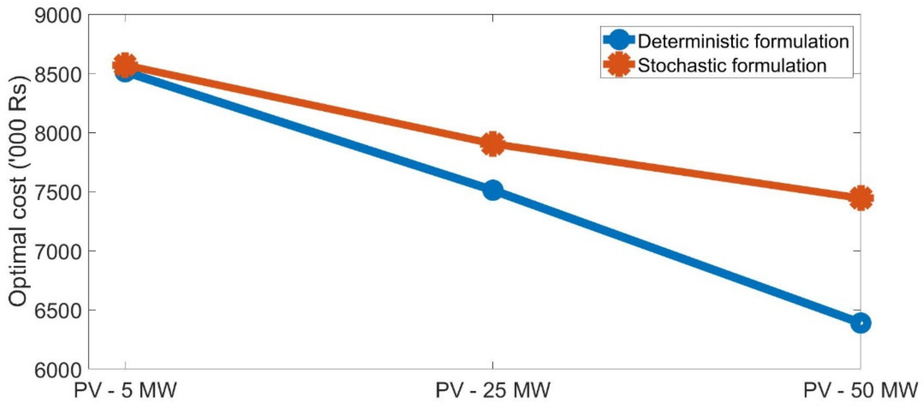
Most of the island economy revolves around the tourism industry. Therefore, load demand is relatively higher in the evenings. A typical PV power output and load profile of South Andaman is shown in Figure 2. Three PV outputs are considered for Figure 2: the existing 5 MWp PV farm and the prospective PV farm of installed capacities 25 MWp and 50 MWp, respectively. It may be easily observed that for 5 MWp and 25 MWp PV farms, the PV output is lower than the load demand profile, whereas the PV output for 50 MWp PV farm is higher than the load demand. Hence, the significance of BESS is far more substantial in the case of the 50 MWp PV plant as compared to the others. However, this does not eliminate the requirement of BESS for the other two cases, as will be evident in Section 3.2.1.
In this work, load demand is represented by point forecasts, while PV power forecasts are treated as a stochastic process with the scenario-based probabilistic forecast. The lower bound, upper bound, and mean PV forecast for a specific day’s prediction is shown in Figure 3. It shows the available range of PV power realization scenarios considered in this work.

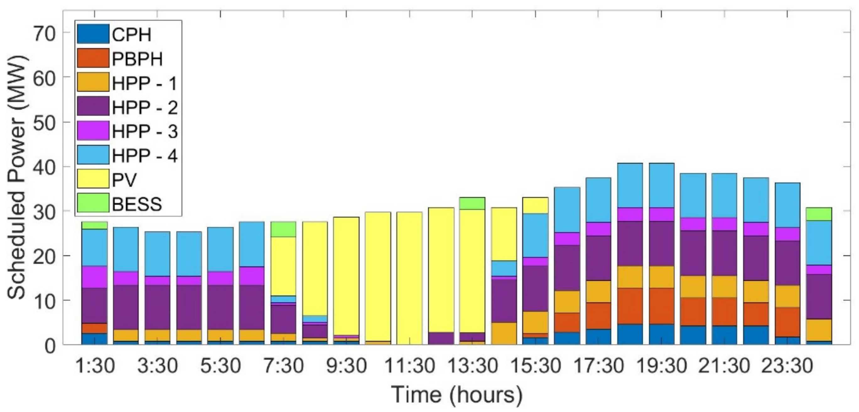
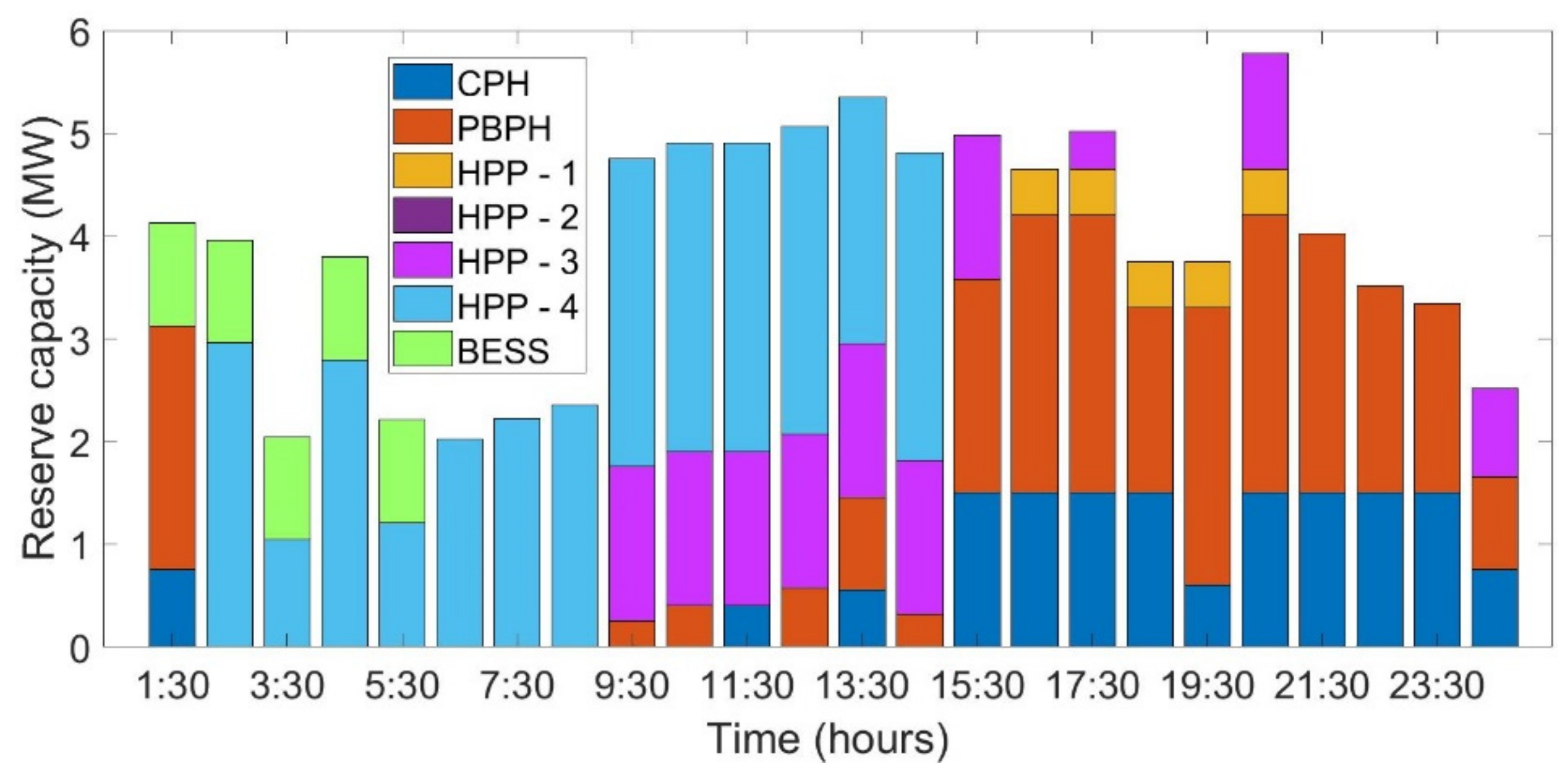
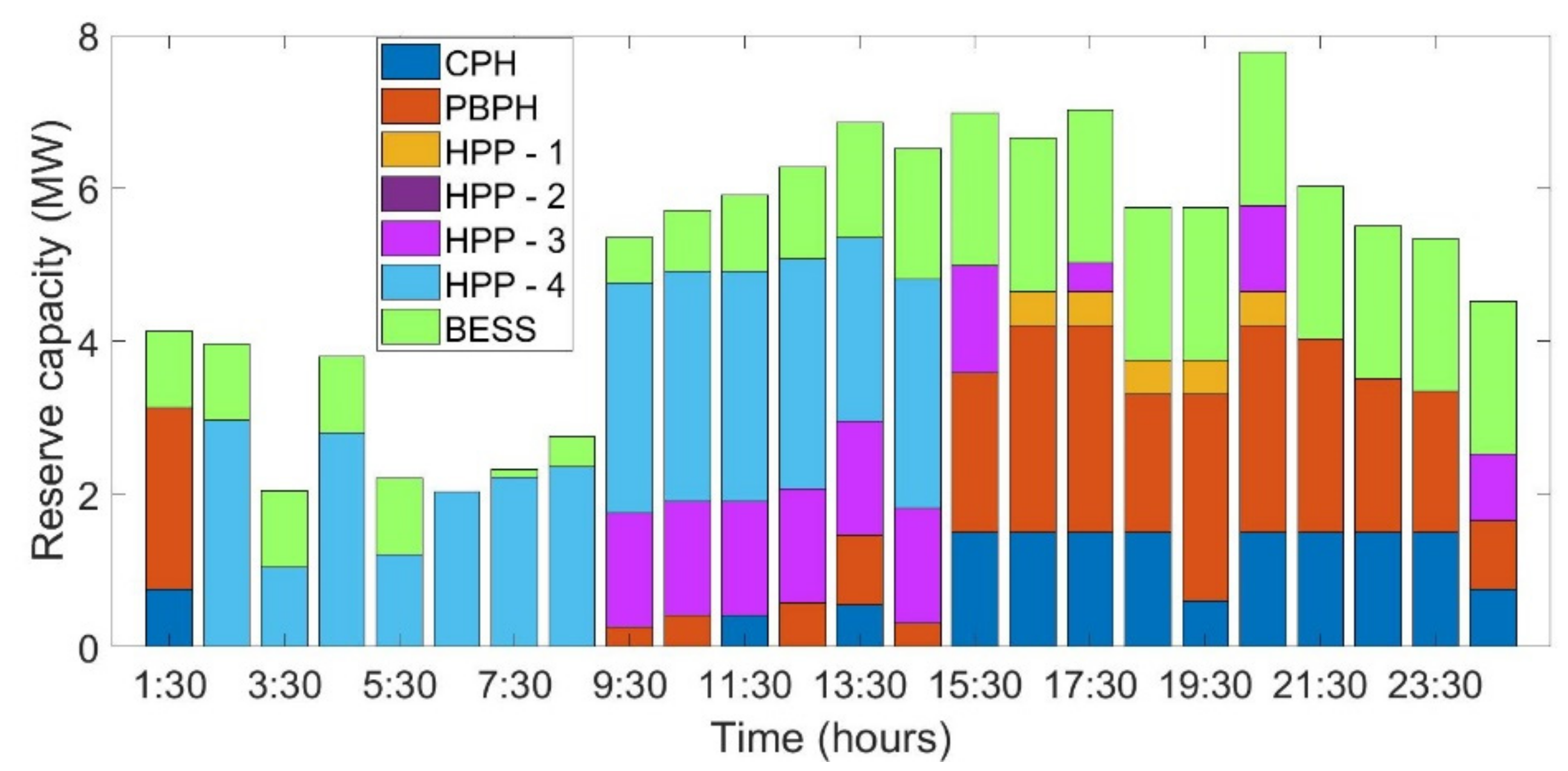
3.2.1. Generation Scheduling Results of the Proposed Model and its Analysis

Generation scheduling of South Andaman Island is managed by the electricity department (A&N Administration). As per the current policy, HPP has a contractual agreement to meet the generation and capacity requirements in peak hours, while the power plants operated by the Electricity Department would supply the remaining power to meet system demand and maintain grid stability. In this work, to make the mathematical formulation relevant for most insular grids, the authors have assumed that generation scheduling is based on day-ahead markets wherein the marginal costs of different generating plants and other network and unit constraints are the deciding factors that determine the generation schedule for each day.
Six different case studies are considered to study the problem from different perspectives. These are listed below. As seen below, the first three case studies, C 1 a , C 2 a , and C 3 a , consider the existing DGPH coupled with PV and BESS of different installed capacities. In the last three cases, C 4 a , C 5 a , and C 6 a , the underlying assumption is that all DGs (except two DGs of 5 MW capacity each) are replaced by a 50 MW LNG-based power plant. All these six cases were analyzed, and their results are presented in the rest of the Subsection.
Case C 1 a : 16 DG + 5 MW PV + 2 MWh BESS
Case C 2 a : 16 DG + 25 MW PV + 12 MWh BESS
Case C 3 a : 16 DG + 50 MW PV + 20 MWh BESS
Case C 4 a : 50 MW LNG + 5 MW PV + 2 MWh BESS
Case C 5 a : 50 MW LNG + 25MW PV + 12MWh BESS
Case C 6 a : 50 MW LNG + 50MW PV + 20MWh BESS
The generation schedule of 24 h for case studies C 1 a , C 2 a , and C 3 a are as shown in Figure 4, Figure 5 and Figure 6. It is observed that the scheduled PV power increases as the installed capacity of the PV power plant increases. On the other hand, the discharging schedule of BESS is close to negligible in cases C 1 a and C 2 a . Further, whatever little is scheduled is only because of the initial assumption that 1 MWh and 5 MWh BESS capacity was available from the previous day’s charging. Even in the case of C 3 a , which has a 50 MWp installed capacity of PV and 20 MWh BESS facility, the actual discharging of power is very small comparatively. This is due to the fact that utilization of BESS is predominantly visible in the up- and down-reserve capacity.
Reserve capacity for cases C 1 a , C 2 a , and C 3 a is as shown in Figure 7, Figure 8 and Figure 9, respectively. In (23) and (24), the here-and-now terms, R i t U and R i t D , and wait-and-see term, P t ω B , are responsible for satisfying the reserve needed to cater to α % variation in load demand and β % variation in scheduled PV power output. Load demand for all the three cases, C 1 a , C 2 a , and C 3 a , will be the same. However, the scheduled PV power output will change with respect to the installed capacity of the PV plant. Current charging status of BESS, as seen in Figure 7, Figure 8 and Figure 9, changes with each scenario of PV power realization. Thus, BESS plays a significant role in a reserve capacity as opposed to energy scheduling. It is to be noted that the reserve provided by BESS will be different for each PV power output-realization scenario. In Figure 7, Figure 8 and Figure 9, a specific scenario, ω, is considered. Reserve capacity requirements are fulfilled differently in each scenario.
The reserve capacity for case C 2 a , considering lower bound, mean, and upper bound PV power output realization, is shown in Figure 10, Figure 11 and Figure 12. As seen in Figure 10, for lower-bound power output scenarios from PV, BESS is in a position to offer reserve only based on the initial PV power output. The PV power produced is being utilized for fulfilling load demand and not for charging the battery. Hence, in the lower-bound scenario, BESS is unable to provide reserve once the initial power from the previous day has been scheduled to discharge at 06:30 a.m. (as seen in Figure 5). On the other hand, in Figure 11 and Figure 12, BESS provides reserve even after discharging at 06:30 a.m. since the PV power output realization is different. Unlike the lower-bound scenario, in the mean and upper-bound scenario, PV power output is used to fulfill load demand and is also used for charging BESS. Hence, this charged status makes it possible for the BESS to provide reserve capacity.
The summary of the above analysis is shown in Table 5, wherein the total generation scheduled for conventional power plants (energy and reserve schedule), PV (scheduled power and curtailed power), and BESS discharging schedule is shown in Table 5. It is observed that the contribution of all the power parameters mentioned in cases C 1 a , C 2 a , and C 3 a are similar to those in cases C 4 a , C 5 a , and C 6 a , i.e., there is very little change in the schedule when the transition happens from DG- to LNG-based power plant. A substantial change in generation schedule is visible only when the transition is from a lower PV installed capacity to a higher one. On the other hand, Table 6 shows there is a substantial change in cost when there is a shift from DG- to LNG-based power plants. (It is to be noted that all costs appearing in Table 6 and Table 7 are expressed in INR (Indian Rupees).)
It is seen that the total cost is on the lower side with LNG-based power plants. Further analysis was carried out considering LNG with different PV and BESS penetrations. These case studies are listed below:
Case C 1 b : 50 MW LNG + 5 MW PV + 2 MWh BESS
Case C 2 b : 50 MW LNG + 25 MW PV + 2 MWh BESS
Case C 3 b : 50 MW LNG + 25 MWPV + 12MWh BESS
Case C 4 b : 50 MW LNG + 50 MW PV + 2 MWh BESS
Case C 5 b : 50 MW LNG + 50MW PV + 12MWh BESS
Case C 6 b : 50 MW LNG + 50MW PV + 20MWh BESS
Table 7 and Table 8 show the cost of generation and power scheduled for different energy sources for cases C 1 b , C 2 b , C 3 b , C 4 b , C 5 b , and C 6 b , respectively. It can be seen from Table 7 that there is an appreciable reduction in cost as the size of PV is changed from 5 MW to 25 MW and then to 50 MW, the least costly being case C 6 b with 50 MW LNG-based gas power plant, 50 MWp PV farm, and 20 MW BESS. However, on comparing cases C 5 b and C 6 b , it can be observed that reduction in overall cost (energy, reserve, and start-up cost) is not substantial when the size of BESS is increased from 12 MW to 20 MW.
A similar observation is seen in Table 8. The utilization of PV and BESS combined increases as the installed capacity of the PV farm increases. However, there is no substantial difference between cases C 5 b and C 6 b , wherein the combined utilization of PV and BESS is almost the same for both cases. The power scheduled for the conventional generation is almost the same for cases C 5 b and C 6 b , which means that the GHG levels will be almost the same for either of the cases. Hence, since there is neither cost-benefit nor GHG level improvement, case C 5 b would be a preferred option as compared to C 6 b , as the investment cost of an additional 10 MWh capacity BESS can be avoided.

3.3. Quality Metrics for Studying the Stochastic Formulation

The proposed model was formulated using a stochastic approach based on the recourse framework. If, for the same system, a deterministic model was to be evaluated with mean forecasts acting as point forecasts for the PV power output, then the objective function value of the deterministic formulation and stochastic formulation (considering first-stage variables only) is as seen in Figure 13 for cases C 4 a (PV—5 MW), C 5 a (PV—25 MW), and C 6 a (PV—50 MW). It is observed that the stochastic cost is always more than the deterministic cost. This is justifiable by the fact that by relying on a stochastic formulation, the reserve cost applicable after actual realization in real-time would be relatively lower than the deterministic schedule due to the fact that stochastic formulations consider a wide range of forecast scenarios with different probabilities as opposed to a deterministic formulation, which considers only the mean forecast.
The stochastic formulation can also be justified through the three other quality metrics, which are defined below. They also help in understanding the conflict introduced by the presence of RES, such as PV. The presence of PV farms leads to the reduction of power generation costs since the economic PV power output would replace some of the power produced by the expensive DGPH. However, the dynamism involved in PV power outputs would result in the rise of reserve power costs.
The following three quality metrics have been used to discuss the conflict between falling generation costs and rising reserve costs of DGPH based on the work presented in [27] for wind farms.
(i)
Average Benefit (AB): AB is defined as the decrease in the expected cost for every additional MWh injected by PV farm into the network. It is mathematically represented as seen in (31). Here, D C t N i l _ P V represents the total optimal cost of the system with no PV farms obtained from a deterministic formulation, while E C t o p t i m a l represents the sum of the first-stage energy, reserve, and start-up cost obtained from the stochastic formulation.
A B = t = 1 N t D C t N i l _ P V E C t o p t i m a l P t ω S N t
(ii)
Average Uncertainty Cost (AUC): AUC is a measure of the equivalent deterministic cost of a system that has the perfect information of the stochastic variable; i.e., PV power output is exactly the same as the mean forecast of the power from PV. It is represented by (32). Here, D C t P I is the optimal objective function value of the system as obtained from a deterministic formulation with perfect information of the PV forecast.
A U C = t = 1 N t E C t o p t i m a l D C t P I P t ω S N t
(iii)
Net Average Benefit (NAB): NAB is the measure of the profitability of the PV power injected into the system. It is represented by (33).
N A B = A B A U C
The values of these metrics were evaluated for the cases C 4 a , C 5 a , and C 6 a . Figure 14 shows the A B and A U C for the abovementioned cases, and the gap between the A B and A U C points represent the N A B of the respective case. It is observed that A U C is always less than A B , and hence, there is a positive N A B present at all times, which justifies the implementation of stochastic formulation for generation scheduling of insular grids with high penetration of PV and BESS.

3.4. Computational Performance of the Proposed Model

The number of variables, equality constraints, and inequality constraints for the mathematical formulation, discussed in Section 2, is given by the following expressions:
(i)
Number of variables = N t 5 N i 1 + N ω + N s 3 + 5 N ω
(ii)
Number of equality constraints = N t 1 + N ω 2 + N i + N s
(iii)
Number of inequality constraints = N t 5 N i 1 + N ω + N s 1 + 5 N ω
These determine the size of the problem. Different case studies have been considered for analyzing the performance of the proposed model. Table 9 shows the problem dimension for the most basic scenario for cases C 1 a , C 2 a , C 3 a , C 4 a , C 5 a , and C 6 a . In the case of C 1 a , C 2 a , and C 3 a , the number of conventional generators, N i , is higher, while in the case of
C 4 a , C 5 a , and C 6 a , they are drastically reduced. Hence, the dimensions of the problem are accordingly impacted, which results in an increasing impact on the time taken to execute the problem.
To study the growth of problem dimension with respect to several scenarios, N ω , three cases of reduced scenarios were studied. These cases considered 10, 25, and 50 equiprobable scenarios, respectively. Computational performance for the same is as shown in Table 9.
Similar to Table 9, in Table 10, the time taken also increases exponentially with the increasing stature of the problem dimension. This is often referred to as the “curse of dimensionality”, which is one of the biggest concerns of stochastic formulations. This is generally true for large complex interconnected systems with more generators and other system parameters and too many forecast scenarios. However, for insular systems, the number of generators is much more limited, and its network configuration is more straightforward. Hence, if the forecast scenarios are obtained through scenario reduction techniques, stochastic approaches can be adopted in insular systems.

4. Concluding Remarks

In this work, a two-stage stochastic generation scheduling model is proposed for an insular grid with high penetration of PV. Proposed stochastic constraints include technical constraints that represent the interplay between RES, such as PV, and energy storage technologies, such as BESS. It also includes system and individual generator reserve constraints that can provide reserve cushion for variabilities introduced by PV. Charging/discharging limit of BESS and other non-anticipatory constraints are also proposed that ensure the technical feasibility of generation schedules of conventional generators, PV, and BESS. The proposed model was validated on the insular grid of South Andaman Island. The results show that the proposed model allows sound scheduling decisions that are technically viable and, at the same time, economically optimal. It shows that PV predominantly contributes to energy scheduling, while BESS does so for the reserve schedules. Results also demonstrate that for the case of South Andaman’s grid, there is sufficient motivation for increasing solar penetration from 5 MWp to 50 MWp, as planned by the government of India, but there is very little reason for increasing the size of BESS from the priory proposed 12 MWh capacity to the newly proposed 25 MWh capacity (based on the techno-commercial assumptions made in this paper) since it was found that increasing BESS capacity neither reduces the overall energy and reserve scheduling costs, nor does it reduce GHG emissions level significantly. The future scope of work would involve changing the perspective of the analysis from the system operator’s point of view to that of the producers and retail consumers’ point of view, who are the primary electricity market participants.

Author Contributions

Conceptualization, L.H., B.A. and A.V.S.; methodology, L.H.; software, L.H.; formal analysis, L.H. and B.A.; writing—original draft preparation, L.H., B.A. and A.V.S.; writing—review and editing, L.H., B.A., A.V.S. and P.M.; visualization, L.H. and P.M.; supervision, B.A. and P.M.; funding acquisition, B.A. All authors have read and agreed to the published version of the manuscript.

Funding

This research work is supported in part by the European Commission H2020 TWINNING Joint Universal activities for Mediterranean PV integration Excellence (JUMP2Excel) project under grant 810809.

Institutional Review Board Statement

Not applicable.

Informed Consent Statement

Not applicable.

Data Availability Statement

The data presented in this study are available on request from the corresponding author.

Acknowledgments

Authors are thankful to the anonymous reviewers and the editors for their suggestions.

Conflicts of Interest

The authors declare no conflict of interest.

References

  1. Ministry of Power. 24 × 7 Power for All—Andaman and Nicobar Islands. 2015. Available online: https://powermin.nic.in/sites/default/files/uploads/joint_initiative_of_govt_of_india_and_andaman_nicobar.pdf (accessed on 15 March 2021).
  2. Sonamothu, K. Energy crisis in Andaman and Nicobar Islands. Int. Adv. Res. J. Sci. Eng. Technol. 2019, 6, 29–35. [Google Scholar]
  3. Duić, N.; Carvalho, M.D.G. Increasing renewable energy sources in island energy supply: Case study Porto Santo. Renew. Sustain. Energy Rev. 2004, 8, 383–399. [Google Scholar] [CrossRef]
  4. Erdinc, O.; Paterakis, N.; Catalão, J.P.S. Overview of insular power systems under increasing penetration of renewable energy sources: Opportunities and challenges. Renew. Sustain. Energy Rev. 2015, 52, 333–346. [Google Scholar] [CrossRef] [Green Version]
  5. Prina, M.G.; Groppi, D.; Nastasi, B.; Garcia, D.A. Bottom-up energy system models applied to sustainable islands. Renew. Sustain. Energy Rev. 2021, 152, 111625. [Google Scholar] [CrossRef]
  6. Gupta, J. NTPC Plans 50 MW Solar Power Plant for the Andamans. Available online: https://timesofindia.indiatimes.com/city/kolka-ta/ntpcplans-50mw-solar-power-plant-for-the-andamans/articleshow/54978188.cms (accessed on 15 March 2021).
  7. Chakrabarti, S.; Heistrene, L.; Amin, A.; Choraria, N. Impact of increasing penetration of renewables in insular grids: Insights from the case of Andaman and Nicobar Islands. In Recent Advances in Power Systems; Springer: Singapore, 2022; pp. 705–714. [Google Scholar] [CrossRef]
  8. Hussain, E.K.; Thies, P.R.; Hardwick, J.; Connor, P.M.; Abusara, M. Grid Island energy transition scenarios assessment through network reliability and power flow analysis. Front. Energy Res. 2021, 8, 584440. [Google Scholar] [CrossRef]
  9. Notton, G. Importance of islands in renewable energy production and storage: The situation of the French islands. Renew. Sustain. Energy Rev. 2015, 47, 260–269. [Google Scholar] [CrossRef]
  10. Diagne, M.; David, M.; Lauret, P.; Boland, J.; Schmutz, N. Review of solar irradiance forecasting methods and a proposition for small-scale insular grids. Renew. Sustain. Energy Rev. 2013, 27, 65–76. [Google Scholar] [CrossRef] [Green Version]
  11. Lu, Z.; Lu, S.; Li, Q.; Zhang, Y. Optimal day-ahead scheduling of islanded microgrid considering risk-based reserve decision. J. Mod. Power Syst. Clean Energy 2021, 9, 1149–1160. [Google Scholar] [CrossRef]
  12. Katsaprakakis, D.; Dakanali, I. Comparing electricity storage technologies for small insular grids. Energy Procedia 2019, 159, 84–89. [Google Scholar] [CrossRef]
  13. Papadopoulos, A.M. Renewable energies and storage in small insular systems: Potential, perspectives and a case study. Renew. Energy 2020, 149, 103–114. [Google Scholar] [CrossRef]
  14. Krishnamoorthy, M.; Periyanayagam, A.D.V.R.; Kumar, C.S.; Kumar, B.P.; Srinivasan, S.; Kathiravan, P. Optimal sizing, selection, and techno-economic analysis of battery storage for PV/BG-based hybrid rural electrification system. IETE J. Res. 2020, 1–16. [Google Scholar] [CrossRef]
  15. Psarros, G.; Nanou, S.; Papaefthymiou, S.V.; Papathanassiou, S.A. Generation scheduling in non-interconnected islands with high RES penetration. Renew. Energy 2018, 115, 338–352. [Google Scholar] [CrossRef]
  16. Sigrist, L.; Lobato, E.; Rouco, L. Energy storage systems providing primary reserve and peak shaving in small isolated power systems: An economic assessment. Int. J. Electr. Power Energy Syst. 2013, 53, 675–683. [Google Scholar] [CrossRef]
  17. Psarros, G.N.; Papathanassiou, S.A. Internal dispatch for RES-storage hybrid power stations in isolated grids. Renew. Energy 2020, 147, 2141–2150. [Google Scholar] [CrossRef]
  18. Ntomaris, A.V.; Bakirtzis, E.A.; Chatzigiannis, D.I.; Simoglou, C.K.; Biskas, P.N.; Bakirtzis, A.G. reserve quantification in insular power systems with high wind penetration. In Proceedings of the IEEE PES Innovative Smart Grid Technologies Europe Conference, Istanbul, Turkey, 12–15 October 2014; pp. 1–6. [Google Scholar] [CrossRef]
  19. Marocco, P.; Ferrero, D.; Martelli, E.; Santarelli, M.; Lanzini, A. An MILP approach for the optimal design of renewable battery-hydrogen energy systems for off-grid insular communities. Energy Convers. Manag. 2021, 245, 114564. [Google Scholar] [CrossRef]
  20. Psarros, G.N.; Dratsas, P.A.; Papathanassiou, S.A. A comparison between central- and self-dispatch storage management principles in island systems. Appl. Energy 2021, 298, 117181. [Google Scholar] [CrossRef]
  21. Simoglou, C.K.; Bakirtzis, E.A.; Biskas, P.N.; Bakirtzis, A.G. Optimal operation of insular electricity grids under high RES penetration. Renew. Energy 2016, 86, 1308–1316. [Google Scholar] [CrossRef]
  22. Ntomaris, A.; Bakirtzi, A. Stochastic scheduling of hybrid power stations in insular power systems with high wind penetration. IEEE Trans. Power Syst. 2016, 31, 3424–3436. [Google Scholar] [CrossRef]
  23. Guillamona, A.; Sarasuab, J.; Chazarrab, M.; Rodriguez, A.; Munozb, D.; Garciaa, A. Frequency control analysis based on unit commitment scheme with high wind power integration: A Spanish isolated power system case study. Electr. Power Energy Syst. 2020, 121, 106044. [Google Scholar] [CrossRef]
  24. Osório, G.J.; Shafie-Khah, M.; Lujano-Rojas, J.M.; Catalão, J.P.S. Scheduling model for renewable energy sources integration in an insular power system. Energies 2018, 11, 144. [Google Scholar] [CrossRef] [Green Version]
  25. Integration Study for Stabilized Grid Operation in Andaman and Nicobar Islands; TERI: Mithapur, India, 2020.
  26. Takyar, S. Waves of Change. Available online: https://renewablewatch.in/2020/09/29/waves-of-change/ (accessed on 15 March 2021).
  27. Conejo, A.; Carrion, M.; Morales, J. Decision Making under Uncertainty in Electricity Markets, 1st ed.; International Series in Operation Research and Management Science; Springer: Boston, MA, USA, 2014. [Google Scholar]
Figure 1. Scenario tree of the proposed model.
Energies 15 02612 g001
Figure 2. Average demand and PV forecast for April 2019 (South Andaman).
Energies 15 02612 g002
Figure 3. Lower and upper bounds of power forecast from PV for 50 MWp solar farm for April 2019.
Energies 15 02612 g003
Figure 4. Day-ahead generation schedule for case C 1 a .
Energies 15 02612 g004
Figure 5. Day-ahead generation schedule for case C 2 a .
Energies 15 02612 g005
Figure 6. Day-ahead generation schedule for case C 3 a .
Energies 15 02612 g006
Figure 7. Reserve capacity schedule for case C 1 a for a specific scenario, ω.
Energies 15 02612 g007
Figure 8. Reserve capacity schedule for case C 2 a for a specific scenario, ω.
Energies 15 02612 g008
Figure 9. Reserve capacity schedule for case C 3 a for a specific scenario, ω. The reserve capacity for case C 2 a .
Energies 15 02612 g009
Figure 10. Reserve capacity schedule for case C 2 a for the lower-bound scenario.
Energies 15 02612 g010
Figure 11. Reserve capacity schedule for case C 2 a for the mean scenario.
Energies 15 02612 g011
Figure 12. Reserve capacity schedule for case C 2 a for the upper-bound scenario.
Energies 15 02612 g012
Figure 13. Deterministic and stochastic costs for cases C 4 a , C 5 a , and C 6 a .
Energies 15 02612 g013
Figure 14. A B , A U C , and N A B for cases C 4 a , C 5 a , and C 6 a .
Energies 15 02612 g014
Table 1. Comparison of recently proposed optimal scheduling strategies for insular grids.
Ref.RES TypeRES
Uncertainty Is Considered
Approach for
Modeling Uncertainty
Model TypeStorage Tech
Involved
Gen. Scheduling Model Is Meant for SOProposed Modification in the Generation Scheduling Problem BESS
Included or Not in Reserve Constraint?
Modelling of Constraint Representing Coordination
between BESS and RES
[15]Wind + PVNoNot
applicable (NA)
MILPNoYesReserve (primary, secondary, and tertiary) NoNo
[16]WindNoNAMILPYesYesReserve; charging and discharging limits of BESSYes (BESS)No
[17]Wind + PVNoNAMILPYesNoNANANA
[18]WindYesTwo-stage
stochastic
MILPNoYesSynchronization, soak phase, and de\synchronization phase constraints; NoNo
[19]PVNoNAMILPYesYesObjective function includes degradation of battery and H2-based devicesYesNo
[20]WindNoNAMILPYesYesNAYesNo
[21]Wind + PVNoMonte CarloNot specifiedYesYesNANoNo
[22]WindYesTwo-stage
stochastic
MILPNoYesSynchronization, soak phase, and desynchronization phase constraints; Yes (pumped storage)No
[23]WindNoNAMILPNoYesFrequency controlNoNo
[24]Wind + PVNoNAMILPNoYes-NoNo
Proposed modelPVYesTwo-stage stochasticMILPYesYesConstraints representing PV and BESS coordination, reserve, and BESS limitsYes (BESS)Yes
Table 2. Nomenclature of the indices and variables.
IndicesPhysical Meaning
t Index for time interval
i Index for conventional generator
ω Index for forecast scenario of power from PV
First-stage
variables
Physical meaning
C i t S U First-stage start-up cost associated with conventional generator, i , at time, t
P i t G Power scheduled for conventional generator, i , at time, t
R i t U Up-reserve capacity offered by conventional generator, i , at time, t
R i t D Down-reserve capacity offered by conventional generator, i , at time, t
P t S s c h Power scheduled for PV at time, 𝑡
P t B d i s Power discharged by BESS at time, 𝑡
u i t First-stage binary variable associated with commitment status of conventional generator, i , at time, t
u t B d i s First-stage binary variable associated with BESS’ discharging status at time, 𝑡
Second-stage
variables
Physical meaning
C i t ω S U Second-stage start-up cost associated with conventional generator, i , at time, t , for scenario, ω
C i t ω A Variable associated with the anticipatory constraint that relates first- and second-stage start-up variables conventional generator, i , at time, t , for scenario, ω
r i t ω U Up-reserve potential associated with conventional generator, i , at time, t , for scenario, ω
r i t ω D Down-reserve potential associated with conventional generator, i , at time, t ,   for scenario, ω
P t ω B Power status of BESS at time, t , for scenario, ω
P t ω B c h g Power consumption during charging of BESS at time, 𝑡, for scenario, ω
P t ω S c u r Power obtained from PV curtailed at time, t , for scenario, ω
v i t ω Second-stage binary variable associated with commitment status of conventional generator, i , at time, 𝑡, for scenario, ω
v t ω B c h g Second-stage binary variable associated with BESS charging status at time, 𝑡, for scenario, ω
r i t ω G Term associated with the anticipatory constraint that relates up- and down-reserve potential variables
C t ω p e n Penalty term associated with the penalties due to curtailment of power from PV and load not served
ParametersPhysical meaning
N t Total time interval
N i Total number of conventional generators
N ω Total number of forecast scenarios
λ i t G Cost of power offered by conventional plant, 𝑖, at time, 𝑡
λ i t R U Cost of up-reserve offered by conventional generator, 𝑖, at time, 𝑡
λ i t R D Cost of down-reserve offered by conventional generator, 𝑖, at time, 𝑡
λ i S U Start-up cost for conventional generator, 𝑖, at time, 𝑡
π ω Probability of forecast scenario, ω
P t D Load demand of the system predicted for time interval, 𝑡
P i m i n Minimum generation capacity of conventional generator, 𝑖
P i m a x Maximum generation capacity of conventional generator, 𝑖
P t ω S Probabilistic forecast of PV at time, 𝑡, for scenario, ω
F t S m i n Lower bound of the power forecast scenarios of PV at time, 𝑡
F t S m a x Upper bound of the power forecast scenarios of PV at time, 𝑡
R i U m a x Maximum up-reserve limit of conventional generator, 𝑖
R i D m a x Maximum down-reserve limit of conventional generator, 𝑖
η c h a g Charging efficiency of BESS
η d i s Discharging efficiency of BESS
Table 3. Full form of acronyms.
AcronymsPhysical Meaning
A&NAndaman and Nicobar
PV
HPP
Photovoltaic system
Hiring power plant
BESSBattery energy storage system
GHGGreenhouse gas
RESRenewable energy sources
DGDiesel generator
DGPHDiesel generator power house
CPHChatham power house
PBPHPhoenix Bay power house
Table 4. Techno-commercial details of diesel generators.
UnitMin. Gen. (MW)Max. Gen. (MW)Gen. Cost
  ( × 10 3   I N R )
Start - Up   Cos t   ( × 10 3   I N R ) Reserve   Cos t   ( × 10 3   I N R )
CPH10.752.52.501802.70
CPH20.752.52.501802.70
CPH30.752.52.501802.70
PBPH10.903.03.001802.70
PBPH20.903.03.001802.70
PBPH30.903.03.001802.70
PBPH40.451.518.001802.70
HPP1-10.722.417.051712.56
HPP1-20.722.417.051712.56
HPP2-10.963.217.171722.56
HPP2-20.963.217.171722.56
HPP2-30.963.217.171722.56
HPP3-10.602.017.451752.62
HPP3-21.505.017.451752.62
HPP4-11.505.017.381742.61
HPP4-21.505.017.381742.61
Table 5. Energy and reserve schedule summary for cases C 1 a , C 2 a , C 3 a , C 4 a , C 5 a , and C 6 a .
Case Study P i t G
(MW)
R i t U
(MW)
R i t D
(MW)
P t S s c h
(MW)
P t ω S c u r
(MW)
P t B d i s
(MW)
C 1 a 743.788.8786.1119.82.001.00
C 2 a 660.582.1142.1199.07.505.00
C 3 a 563.348.2439.05190.336.2310.91
C 4 a 743.774.4268.1319.82.001.00
C 5 a 660.516.7444.8496.58.507.50
C 6 a 563.316.9427.20192.432.618.81
Table 6. Energy, start-up, and reserve costs for cases C 1 a , C 2 a , C 3 a , C 4 a , C 5 a , and C 6 a .
Case StudyEnergy Cost
  ( × 10 3   I N R )
Up-Reserve Cost ( × 10 3   I N R ) Down-Reserve Cost ( × 10 3   I N R ) Start-Up Cost
  ( × 10 3   I N R )
Total Cost
  ( × 10 3   I N R )
C 1 a 12,920236147141814,721
C 2 a 11,49021672141813,197
C 3 a 980112767332613,322
C 4 a 83661267708598
C 5 a 747531503477904
C 6 a 6412313211557631
Table 7. Energy, start-up, and reserve costs for cases C 1 b , C 2 b , C 3 b , C 4 b , C 5 b , and C 6 b .
Case StudyEnergy Cost
  ( × 10 3   I N R )
Up-Reserve Cost ( × 10 3   I N R ) Down-Reserve Cost ( × 10 3   I N R ) Start-Up Cost
  ( × 10 3   I N R )
Total Cost
  ( × 10 3   I N R )
C 1 b 83661267708598
C 2 b 7612141923478193
C 3 b 747531503477904
C 4 b 71421811097468179
C 5 b 6501432011557720
C 6 b 6412313211557631
Table 8. Energy and reserve schedule summary for cases C 1 a , C 2 a , C 3 a , C 4 a , C 5 a , and C 6 a .
Case Study P i t G
(MW)
R i t U
(MW)
R i t D
(MW)
P t S s c h
(MW)
P t ω S c u r
(MW)
P t B d i s
(MW)
C 2 b 671.281.381.990.43.0671.2
C 3 b 660.516.744.896.57.5660.5
C 4 b 626.8105.996.3135.91.7626.8
C 5 b 564.820.716.2185.714.0564.8
C 6 b 563.316.927.20192.48.81563.3
Table 9. Computational performance for cases C 1 a , C 2 a , C 3 a , C 4 a , C 5 a , and C 6 a .
Case StudyNo. of
Decision Variables
No. of Equality ConstraintsNo. of Inequality ConstraintsEvaluated NodesTime (s)
C 1 a 81121392793216,788330.5
C 2 a 31,179661.4
C 3 a 139,2197175
C 4 a 18724581692160.1
C 5 a 11082.18
C 6 a 14482.39
Table 10. Problem dimension for different reduced scenario sets.
Sr. No.No. of ScenariosNo. of
Decision Variables
No. of Equality ConstraintsNo. of Inequality ConstraintsTime (s)
11052321464474483
22512,432362411,284634
35024,432722422,1847165
Publisher’s Note: MDPI stays neutral with regard to jurisdictional claims in published maps and institutional affiliations.

