
Machine Learning Methods Modeling Carbohydrate-Enriched Cyanobacteria Biomass Production in Wastewater Treatment Systems

 , , , ,
  and
and 
Abstract
:1. Introduction
- This work uses a dataset with 18 variables affecting carbohydrate accumulation in a mixed cyanobacteria consortium treating real wastewater. This work started with an incomplete dataset for three main reasons: (1) the costs involved in water quality analysis; (2) the fact that an automatic device does not monitor the samples, so an analysis has to be performed on a daily or weekly basis; and (3) water quality analysis generates waste in most of the cases, which generates the need to perform a reconstruction of information.
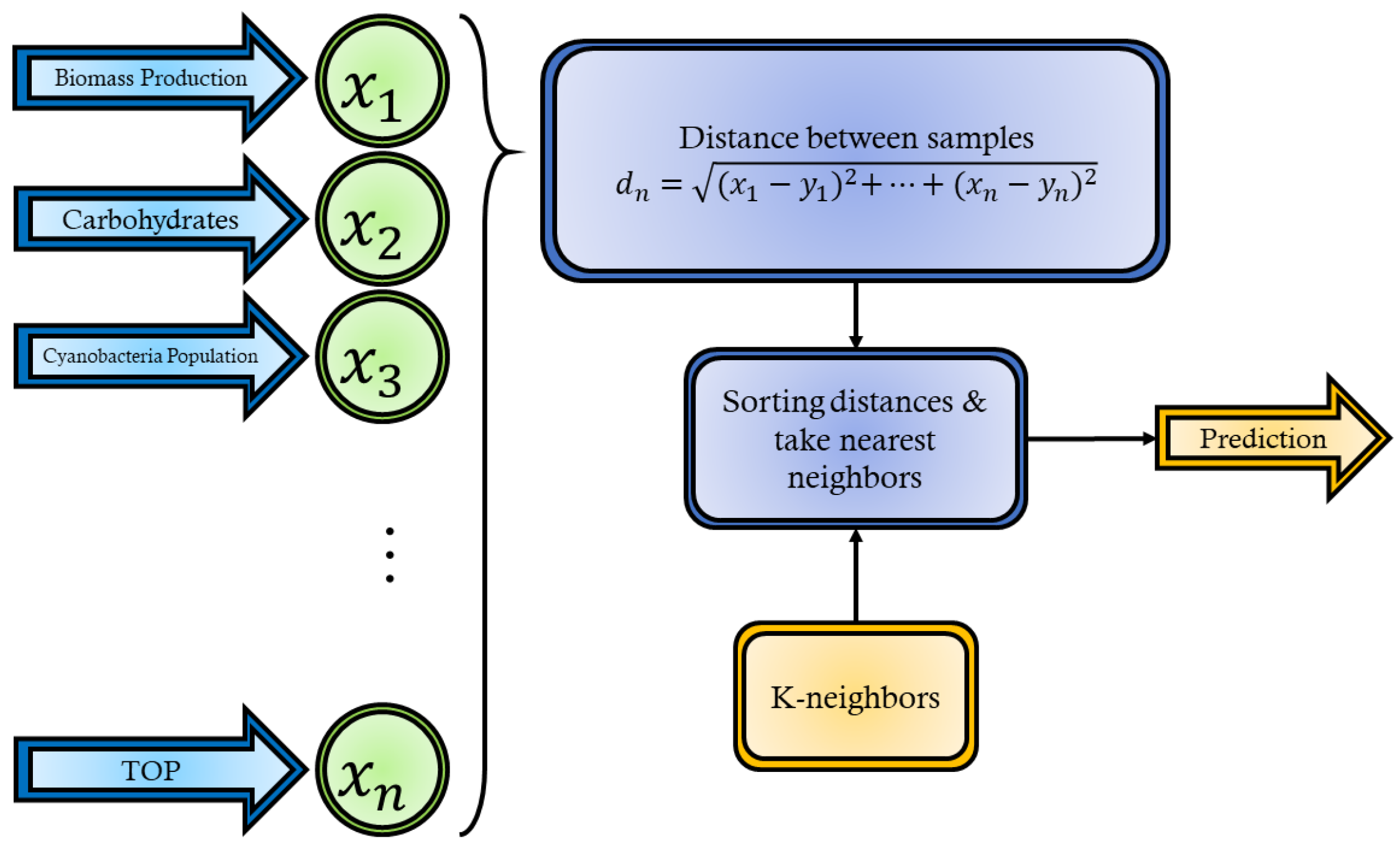
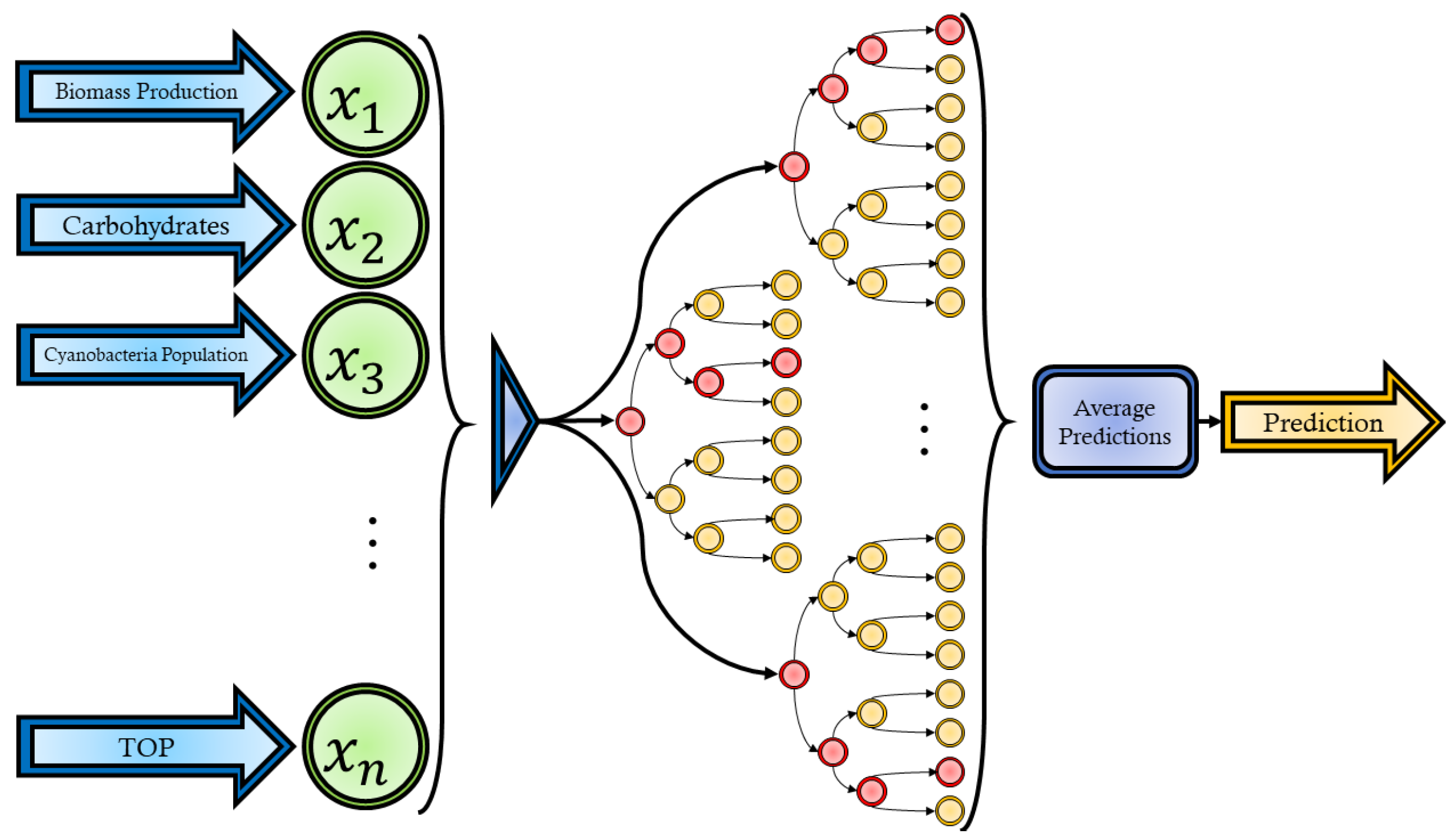
- A trade-off analysis of five learning models of artificial intelligence was carried out using the database of cyanobacterial biomass production in wastewater treatment systems. The five learning models considered were as folows: (1) Artificial Neural Networks (ANNs), (2) Convolutional Neural Networks (CNN), (3) Long Short-Term Memory Network (LSTMs), (4) K-Nearest Neighbors (kNN), and (5) Random Forest (RF)). The AI methods allow learning how the 18 variables of the database interact in order to predict biomass production.
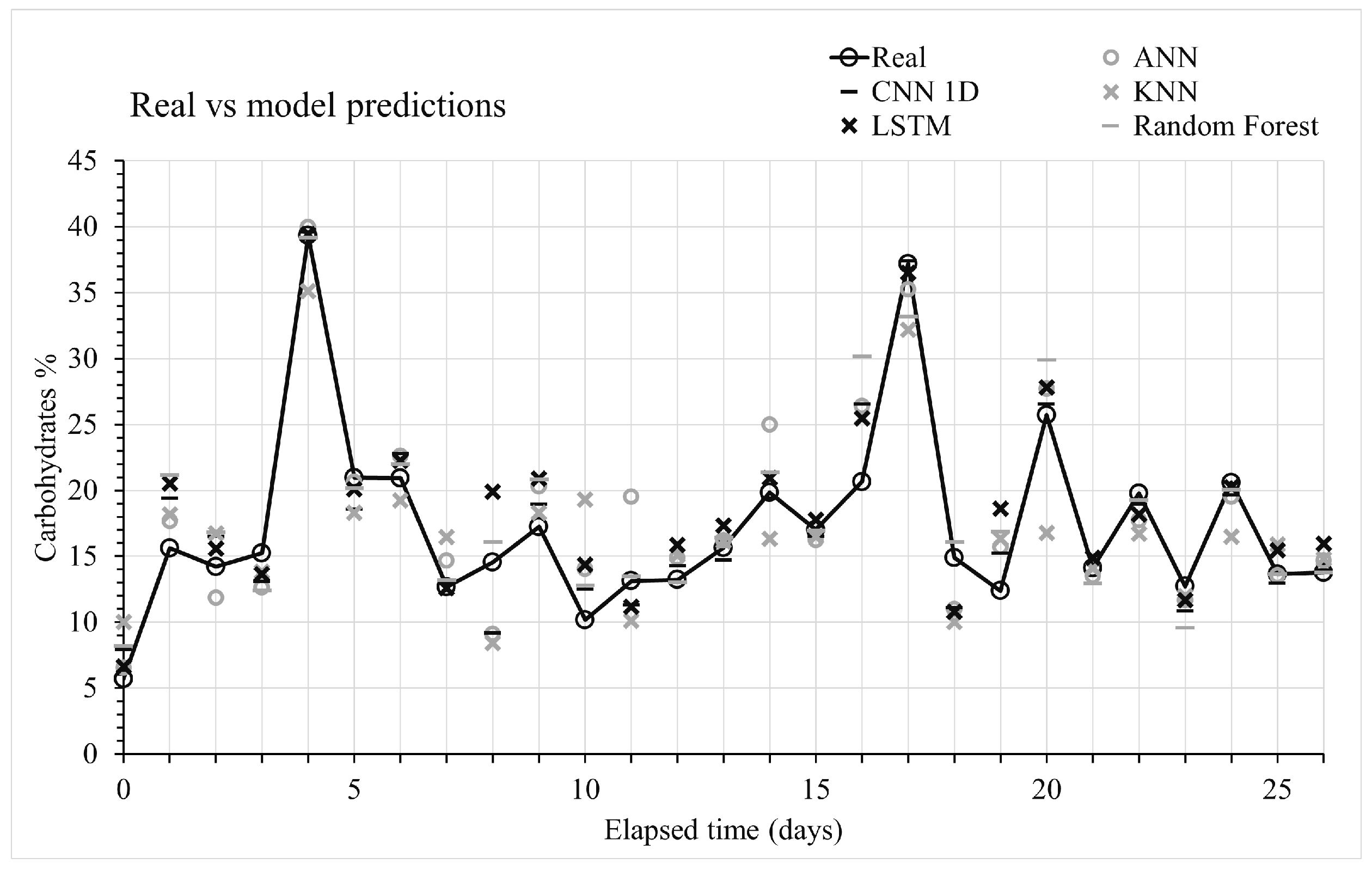
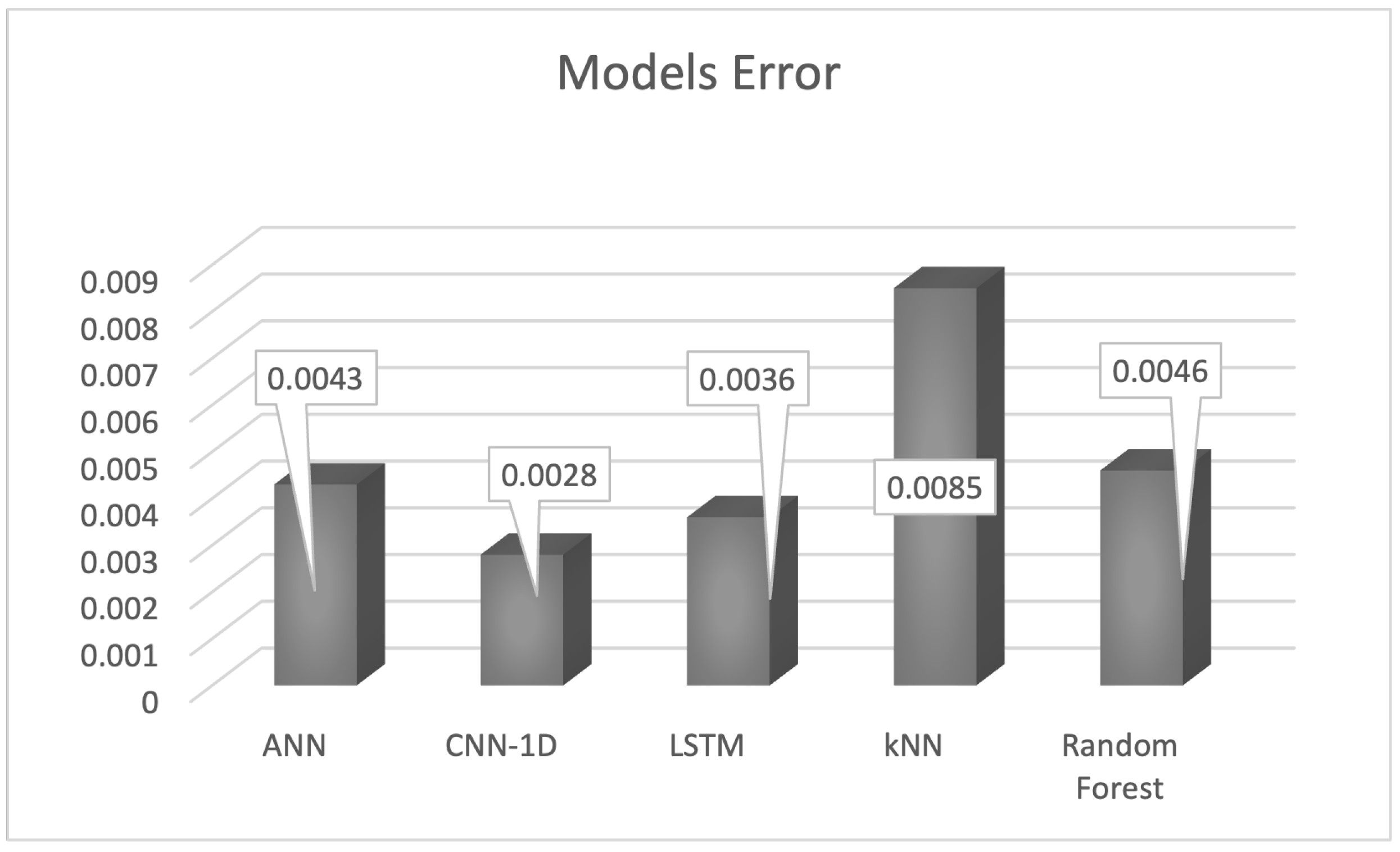
- The best result to predict the biomass production was the CNN-1D model with an MSE (Mean Squared Error) = 0.0028. If a model has an MSE close to zero, it can be concluded that the learning model adequately follows the system’s dynamics.
- By using the forecast model (CNN-1D), several simulations can be generated to evaluate the conditions of experiments that predict the accumulation of carbohydrates, which could reduce sampling analysis, reagents cost, human work, and waste generation.
2. Materials and Methods
2.1. Experimental Data
Microalgae Inoculum and Culture
2.2. Machine Learning Approach Description
2.2.1. Dataset Preparation
2.2.2. Machine Learning Setup
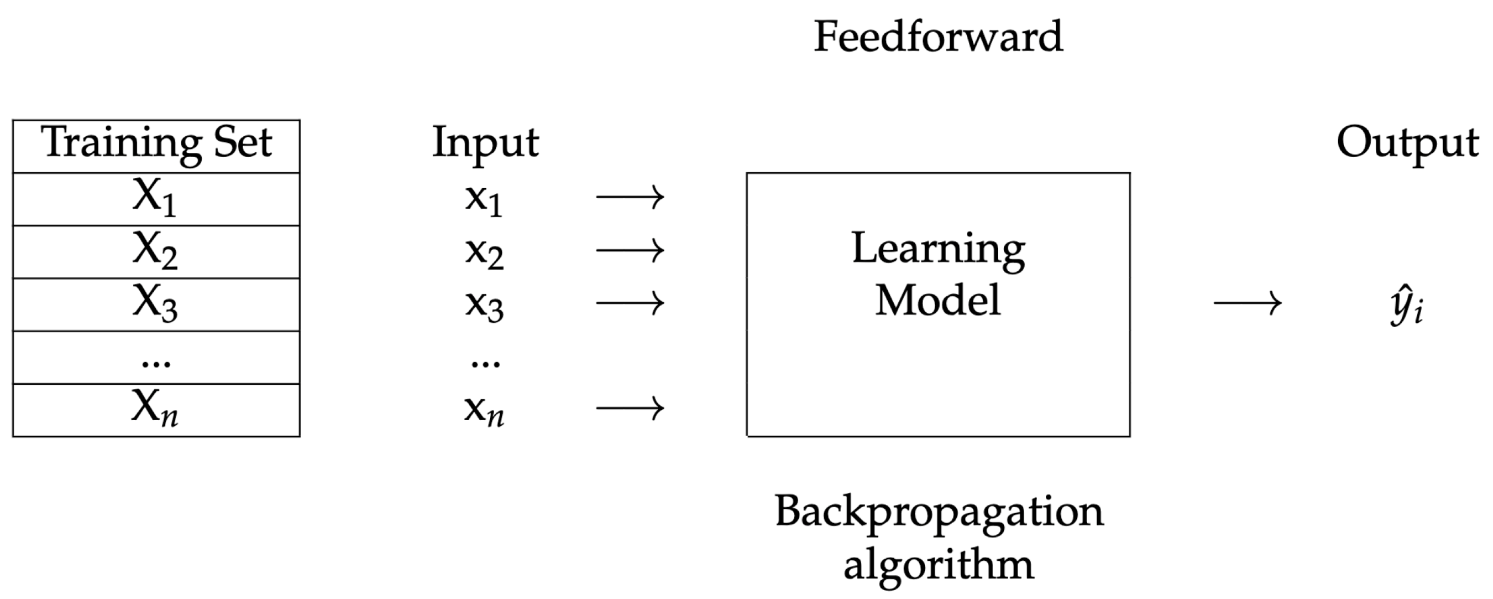
2.2.3. Machine Learning Model Design
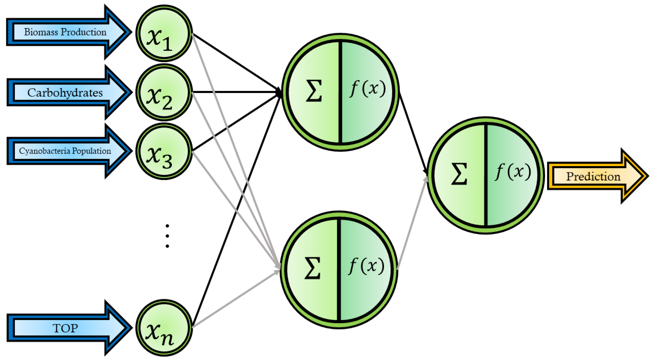
Artificial Neural Network
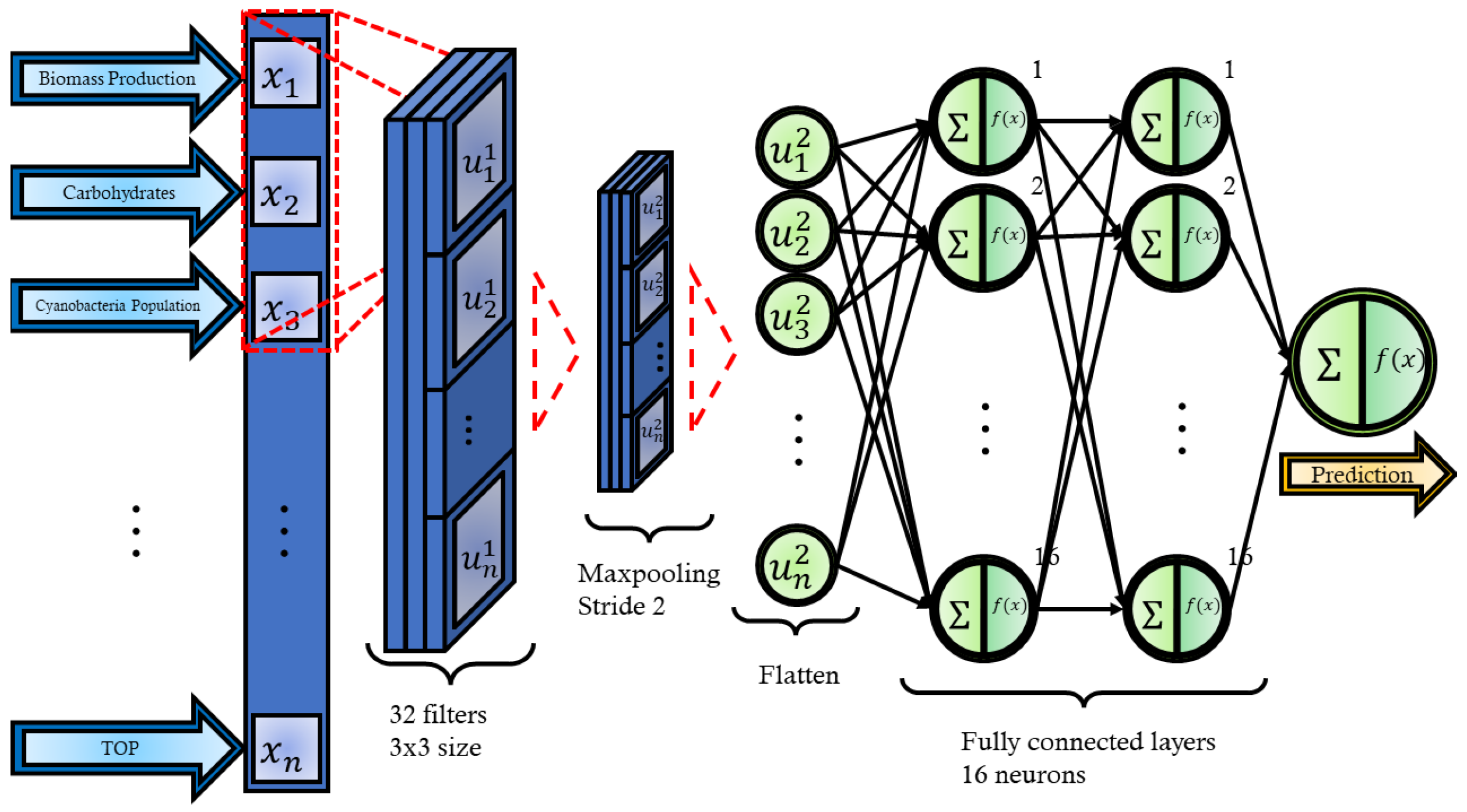
Convolutional Neural Network
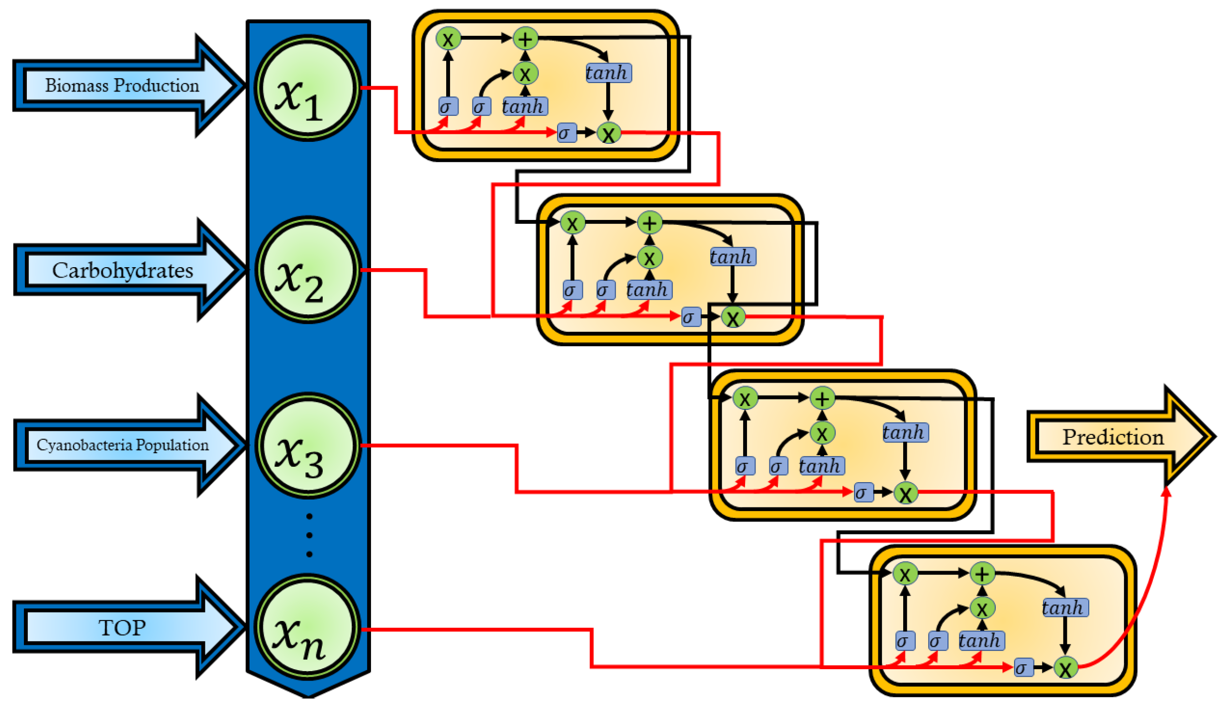
Long Short-Term Memory Network
K-Nearest Neighbors
Random Forest
2.3. Evaluation Metric and Optimization
3. Results
3.1. Experiments Configuration
3.2. Experiments Results
4. Conclusions
Author Contributions
Funding
Institutional Review Board Statement
Informed Consent Statement
Data Availability Statement
Conflicts of Interest
References
- Okoye, P.; Abdullah, A.; Hameed, B. A review on recent developments and progress in the kinetics and deactivation of catalytic acetylation of glycerol—A byproduct of biodiesel. Renew. Sustain. Energy Rev. 2017, 74, 387–401. [Google Scholar] [CrossRef]
- Wang, C.; Luo, D.; Zhang, X.; Huang, R.; Cao, Y.; Liu, G.; Zhang, Y.; Wang, H. Biochar-based slow-release of fertilizers for sustainable agriculture: A mini review. Environ. Sci. Ecotechnol. 2022, 10, 100167. [Google Scholar] [CrossRef]
- Wang, C.; Wang, H. Carboxyl functionalized Cinnamomum camphora for removal of heavy metals from synthetic wastewater-contribution to sustainability in agroforestry. J. Clean. Prod. 2018, 184, 921–928. [Google Scholar] [CrossRef]
- Aitken, D.; Bulboa, C.; Godoy-Faundez, A.; Turrion-Gomez, J.L.; Antizar-Ladislao, B. Life cycle assessment of macroalgae cultivation and processing for biofuel production. J. Clean. Prod. 2014, 75, 45–56. [Google Scholar] [CrossRef]
- Wang, C.; Sun, R.; Huang, R. Highly dispersed iron-doped biochar derived from sawdust for Fenton-like degradation of toxic dyes. J. Clean. Prod. 2021, 297, 126681. [Google Scholar] [CrossRef]
- Huang, Y.; Luo, L.; Xu, K.; Wang, X.C. Characteristics of external carbon uptake by microalgae growth and associated effects on algal biomass composition. Bioresour. Technol. 2019, 292, 121887. [Google Scholar] [CrossRef] [PubMed]
- Arias, D.M.; García, J.; Uggetti, E. Production of polymers by cyanobacteria grown in wastewater: Current status, challenges and future perspectives. New Biotechnol. 2020, 55, 46–57. [Google Scholar] [CrossRef]
- Rizwan, M.; Mujtaba, G.; Memon, S.A.; Lee, K.; Rashid, N. Exploring the potential of microalgae for new biotechnology applications and beyond: A review. Renew. Sustain. Energy Rev. 2018, 92, 394–404. [Google Scholar] [CrossRef]
- de Farias Silva, C.E.; Bertucco, A. Bioethanol from microalgae and cyanobacteria: A review and technological outlook. Process Biochem. 2016, 51, 1833–1842. [Google Scholar] [CrossRef]
- Vargas, S.R.; dos Santos, P.V.; Zaiat, M.; do Carmo Calijuri, M. Optimization of biomass and hydrogen production by Anabaena sp. (UTEX 1448) in nitrogen-deprived cultures. Biomass Bioenergy 2018, 111, 70–76. [Google Scholar] [CrossRef]
- Arias, D.M.; Uggetti, E.; García, J. Assessing the potential of soil cyanobacteria for simultaneous wastewater treatment and carbohydrate-enriched biomass production. Algal Res. 2020, 51, 102042. [Google Scholar] [CrossRef]
- Tóth, P.; Garami, A.; Csordás, B. Image-based deep neural network prediction of the heat output of a step-grate biomass boiler. Appl. Energy 2017, 200, 155–169. [Google Scholar] [CrossRef]
- Rodriguez, H.; Flores, J.J.; Morales, L.A.; Lara, C.; Guerra, A.; Manjarrez, G. Forecasting from incomplete and chaotic wind speed data. Soft Comput. 2019, 23, 10119–10127. [Google Scholar] [CrossRef]
- Guo, H.; Jeong, K.; Lim, J.; Jo, J.; Kim, Y.M.; Park, J.p.; Kim, J.H.; Cho, K.H. Prediction of effluent concentration in a wastewater treatment plant using machine learning models. J. Environ. Sci. 2015, 32, 90–101. [Google Scholar] [CrossRef] [PubMed]
- Rodriguez, H.; Puig, V.; Flores, J.J.; Lopez, R. Flow meter data validation and reconstruction using neural networks: Application to the Barcelona water network. In Proceedings of the 2016 European Control Conference (ECC), Aalborg, Denmark, 29 June–1 July 2016; pp. 1746–1751. [Google Scholar] [CrossRef]
- Granata, F.; Papirio, S.; Esposito, G.; Gargano, R.; De Marinis, G. Machine Learning Algorithms for the Forecasting of Wastewater Quality Indicators. Water 2017, 9, 105. [Google Scholar] [CrossRef] [Green Version]
- Gonzalez-Huitron, V.; León-Borges, J.A.; Rodriguez-Mata, A.E.; Amabilis-Sosa, L.E.; Ramírez-Pereda, B.; Rodriguez, H. Disease detection in tomato leaves via CNN with lightweight architectures implemented in Raspberry Pi 4. Comput. Electron. Agric. 2021, 181, 105951. [Google Scholar] [CrossRef]
- Ali, I.; Greifeneder, F.; Stamenkovic, J.; Neumann, M.; Notarnicola, C. Review of Machine Learning Approaches for Biomass and Soil Moisture Retrievals from Remote Sensing Data. Remote Sens. 2015, 7, 16398–16421. [Google Scholar] [CrossRef] [Green Version]
- Farza, M.; Rodriguez-Mata, A.; Robles-Magdaleno, J.; M’Saad, M. A new filtered high gain observer design for the estimation of the components concentrations in a photobioreactor in microalgae culture. IFAC-PapersOnLine 2019, 52, 904–909. [Google Scholar] [CrossRef]
- Zentou, H.; Zainal Abidin, Z.; Yunus, R.; Awang Biak, D.R.; Zouanti, M.; Hassani, A. Modelling of Molasses Fermentation for Bioethanol Production: A Comparative Investigation of Monod and Andrews Models Accuracy Assessment. Biomolecules 2019, 9, 308. [Google Scholar] [CrossRef] [Green Version]
- Bekirogullari, M.; Pittman, J.K.; Theodoropoulos, C. Multi-factor kinetic modelling of microalgal biomass cultivation for optimised lipid production. Bioresour. Technol. 2018, 269, 417–425. [Google Scholar] [CrossRef]
- Jerono, P.; Schaum, A.; Meurer, T. Observer Design for the Droop Model with Biased Measurement: Application to Haematococcus Pluvialis. In Proceedings of the 2018 IEEE Conference on Decision and Control (CDC), Miami Beach, FL, USA, 17–19 December 2018; pp. 6295–6300. [Google Scholar] [CrossRef]
- Teng, S.Y.; Yew, G.Y.; Sukačová, K.; Show, P.L.; Máša, V.; Chang, J.S. Microalgae with artificial intelligence: A digitalized perspective on genetics, systems and products. Biotechnol. Adv. 2020, 44, 107631. [Google Scholar] [CrossRef] [PubMed]
- Dutta, S.; Madan, S.; Parikh, H.; Sundar, D. An ensemble micro neural network approach for elucidating interactions between zinc finger proteins and their target DNA. BMC Genom. 2016, 17, 1033. [Google Scholar] [CrossRef] [PubMed]
- Linder, J.; Bogard, N.; Rosenberg, A.B.; Seelig, G. A Generative Neural Network for Maximizing Fitness and Diversity of Synthetic DNA and Protein Sequences. Cell Syst. 2020, 11, 49–62. [Google Scholar] [CrossRef] [PubMed]
- Zenooz, A.M.; Ashtiani, F.Z.; Ranjbar, R.; Nikbakht, F.; Bolouri, O. Comparison of different artificial neural network architectures in modeling of Chlorella sp. flocculation. Prep. Biochem. Biotechnol. 2017, 47, 570–577. [Google Scholar] [CrossRef]
- Ruiz-Santaquiteria, J.; Bueno, G.; Deniz, O.; Vallez, N.; Cristobal, G. Semantic versus instance segmentation in microscopic algae detection. Eng. Appl. Artif. Intell. 2020, 87, 103271. [Google Scholar] [CrossRef]
- Treloar, N.J.; Fedorec, A.J.H.; Ingalls, B.; Barnes, C.P. Deep reinforcement learning for the control of microbial co-cultures in bioreactors. PLoS Comput. Biol. 2020, 16, e1007783. [Google Scholar] [CrossRef] [Green Version]
- Andreotti, V.; Solimeno, A.; Rossi, S.; Ficara, E.; Marazzi, F.; Mezzanotte, V.; García, J. Bioremediation of aquaculture wastewater with the microalgae Tetraselmis suecica: Semi-continuous experiments, simulation and photo-respirometric tests. Sci. Total Environ. 2020, 738, 139859. [Google Scholar] [CrossRef]
- Solimeno, A.; Samsó, R.; Uggetti, E.; Sialve, B.; Steyer, J.P.; Gabarró, A.; García, J. New mechanistic model to simulate microalgae growth. Algal Res. 2015, 12, 350–358. [Google Scholar] [CrossRef] [Green Version]
- Figueroa-Torres, G.M.; Pittman, J.K.; Theodoropoulos, C. Kinetic modelling of starch and lipid formation during mixotrophic, nutrient-limited microalgal growth. Bioresour. Technol. 2017, 241, 868–878. [Google Scholar] [CrossRef] [Green Version]
- Federation, W.E.; Association, A. Standard Methods for the Examination of Water and Wastewater; American Public Health Association (APHA): Washington, DC, USA, 2005; Volume 21. [Google Scholar]
- Lin, S. Algal Culturing Techniques. J. Phycol. 2005, 41, 906–908. [Google Scholar] [CrossRef]
- Lanham, A.B.; Ricardo, A.R.; Coma, M.; Fradinho, J.; Carvalheira, M.; Oehmen, A.; Carvalho, G.; Reis, M.A.M. Optimisation of glycogen quantification in mixed microbial cultures. Bioresour. Technol. 2012, 118, 518–525. [Google Scholar] [CrossRef] [PubMed]
- Valenzuela, M. Machine Learning Microalgae. 2021. Available online: https://cvalenzuelab.com/ (accessed on 26 February 2022).
- Patterson, J.; Gibson, A. Deep Learning: A Practitioner’s Approach, 1st ed.; O’Reilly Media, Inc.: Sebastopol, CA, USA, 2017. [Google Scholar]
- Guidici, D.; Clark, M.L. One-Dimensional Convolutional Neural Network Land-Cover Classification of Multi-Seasonal Hyperspectral Imagery in the San Francisco Bay Area, California. Remote Sens. 2017, 9, 629. [Google Scholar] [CrossRef] [Green Version]
- Xiaoyun, Q.; Xiaoning, K.; Chao, Z.; Shuai, J.; Xiuda, M. Short-term prediction of wind power based on deep Long Short-Term Memory. In Proceedings of the 2016 IEEE PES Asia-Pacific Power and Energy Engineering Conference (APPEEC), Xi’an, China, 25–28 October 2016; pp. 1148–1152. [Google Scholar] [CrossRef]
- Al-Qahtani, F.H.; Crone, S.F. Multivariate k-nearest neighbour regression for time series data—A novel algorithm for forecasting UK electricity demand. In Proceedings of the 2013 International Joint Conference on Neural Networks (IJCNN), Dallas, TX, USA, 4–9 August 2013; pp. 1–8. [Google Scholar] [CrossRef]
- Kramer, O. Scikit-Learn; Springer: New York, NY, USA, 2016; pp. 45–53. [Google Scholar]
- Dillon, J.V.; Langmore, I.; Tran, D.; Brevdo, E.; Vasudevan, S.; Moore, D.; Patton, B.; Alemi, A.; Hoffman, M.; Saurous, R.A. Tensorflow distributions. arXiv 2017, arXiv:1711.10604. [Google Scholar]
- He, Y.; Chen, L.; Zhou, Y.; Chen, H.; Zhou, X.; Cai, F.; Huang, J.; Wang, M.; Chen, B.; Guo, Z. Analysis and model delineation of marine microalgae growth and lipid accumulation in flat-plate photobioreactor. Biochem. Eng. J. 2016, 111, 108–116. [Google Scholar] [CrossRef]
- Wang, D.; Lai, Y.C.; Karam, A.L.; de los Reyes, F.L.; Ducoste, J.J. Dynamic Modeling of Microalgae Growth and Lipid Production under Transient Light and Nitrogen Conditions. Environ. Sci. Technol. 2019, 53, 11560–11568. [Google Scholar] [CrossRef]
- Kaplan, E.; Sayar, N.A.; Kazan, D.; Sayar, A.A. Assessment of different carbon and salinity level on growth kinetics, lipid, and starch composition of Chlorella vulgaris SAG 211-12. Int. J. Green Energy 2020, 17, 290–300. [Google Scholar] [CrossRef]
- Murwanashyaka, T.; Shen, L.; Yang, Z.; Chang, J.S.; Manirafasha, E.; Ndikubwimana, T.; Chen, C.; Lu, Y. Kinetic modelling of heterotrophic microalgae culture in wastewater: Storage molecule generation and pollutants mitigation. Biochem. Eng. J. 2020, 157, 107523. [Google Scholar] [CrossRef]
- Gojkovic, Z.; Lu, Y.; Ferro, L.; Toffolo, A.; Funk, C. Modeling biomass production during progressive nitrogen starvation by North Swedish green microalgae. Algal Res. 2020, 47, 101835. [Google Scholar] [CrossRef]
- Packer, A.; Li, Y.; Andersen, T.; Hu, Q.; Kuang, Y.; Sommerfeld, M. Growth and neutral lipid synthesis in green microalgae: A mathematical model. Bioresour. Technol. 2011, 102, 111–117. [Google Scholar] [CrossRef]
- Supriyanto; Noguchi, R.; Ahamed, T.; Rani, D.S.; Sakurai, K.; Nasution, M.A.; Wibawa, D.S.; Demura, M.; Watanabe, M.M. Artificial neural networks model for estimating growth of polyculture microalgae in an open raceway pond. Biosyst. Eng. 2019, 177, 122–129. [Google Scholar] [CrossRef]


| Experiment | HRT/SRT (d) | Dilution Rate Influent a | Volume Removed (L) b | Volume Added (L) c | |
|---|---|---|---|---|---|
| Set 1 | A1 | 10 | 1:1 | 0.25 | 0.25 |
| A2 | 10 | 2:1 | 0.25 | 0.25 | |
| Set 2 | A3 | 8 | 1 | 0.31 | 0.31 |
| A4 | 6 | 1 | 0.42 | 0.42 |
| Experiment | ||||||
|---|---|---|---|---|---|---|
| A1 | A2 | A3 | A4 | |||
| Parameter | Units | Average Value | ||||
| Mixed liquor | Biomass production | g/L·d | 0.04 ± 0.01 | 0.04 ± 0.01 | 0.06 ± 0.01 | 0.05 ± 0.01 |
| Carbohydrates | % | 15.51 ± 11.8 | 23.78 ± 13.82 | 18.20 ± 5.08 | 16.03 ± 6.07 | |
| Cyanobacteria population | Log cell/mL | 11.9 ± 0.01 | 11.91 ± 0.02 | 11.92 ± 0.02 | 11.95 ± 0.04 | |
| Diatom population | Log cell/mL | 9.14 ± 0.39 | 9.24 ± 0.28 | 9.45 ± 0.22 | 9.66 ± 0.28 | |
| Green algae population | Log cell/mL | 8.50 ± 0.37 | 8.43 ± 0.42 | 8.48 ± 0.52 | 8.76 ± 0.46 | |
| Protozoa population | Log cell/mL | 6.93 ± 3.06 | 7.84 ± 0.38 | 7.99 ± 0.19 | 8.15 ± 0.16 | |
| Influent | TIC | mg/L | 71.46 ± 12.25 | 71.46 ± 12.25 | 84.25 ± 6.00 | 84.25 ± 6.00 |
| TOC | mg/L | 161.82 ± 52.5 | 161.83 ± 52.50 | 117.56 ± 25.46 | 117.56 ± 25.46 | |
| TIN | mg/L | 67.5 ± 12.83 | 67.5 ± 13.84 | 65.12 ± 6.87 | 65.12 ± 6.87 | |
| TON | mg/L | 35.18 ± 17.32 | 35.19 ± 17.33 | 19.69 ± 8.91 | 19.69 ± 8.91 | |
| TIP | mg/L | 8.59 ± 3.06 | 8.59 ± 3.07 | 5.22 ± 1.41 | 5.22 ± 1.41 | |
| TOP | mg/L | 5.68 ± 3.08 | 5.69 ± 3.09 | 2.50 ± 1.24 | 2.5 ± 1.24 | |
| Effluent | TIC | mg/L | 4.48 ± 1.48 | 3.58 ± 3.16 | 0.93 ± 3.01 | 2.94 ± 3.78 |
| TOC | mg/L | 22.52 ± 10.32 | 24.06 ± 16.39 | 0.54 ± 1.39 | 2.53 ± 3.47 | |
| TIN | mg/L | 2.10 ± 3.41 | 1.16 ± 1.66 | 21.92 ± 11.42 | 16.17 ± 10.44 | |
| TON | mg/L | 3.40 ± 1.69 | 0 | 0.05 ± 0.15 | 2.33 ± 3.6 | |
| TIP | mg/L | 8.59 ± 3.06 | 0.37 ± 0.83 | 3.72 ± 1.61 | 3.73 ± 1.78 | |
| TOP | mg/L | 0.73 ± 0.82 | 2.41 ± 0.95 | 0.98 ± 1.88 | 0.79 ± 1.23 | |
| Database | |
|---|---|
| … | … |
| Sample | Input | Output | |
|---|---|---|---|
| Training | |||
| data | |||
| 75% | |||
| … | … | … | |
| Validation | … | … | … |
| data | |||
| 25% | |||
| Model | Configurations | Hyperparameters |
|---|---|---|
| ANN | Input layer = 2, relu (input shape = 18) Hidden layer = 20, relu Hidden layer = 20, relu Output layer = 1, sigmoid Optimizer = adam Loss = MSE Metrics = accuracy | Epochs = 1500 Batch size = 16 Verbose = 0 Shuffle = 1 EarlyStop Patience = 20 Monitor loss |
| CNN | Conv1D (filters = 32, kernel size = 3, activation = relu) MaxPooling (pool Size = 2) Flatten() Dense(16, activation = relu) Dense (16, activation = relu) Dense (1, activation = sigmoid) Optimizer = adam Loss = mse Metrics = Accuracy | Epochs = 400 Batch size = 16 Verbose = 0 Shuffle = 1 EarlyStop Patience = 20 Monitor loss |
| KNN | weights = uniform n_neighbors = 5 algorithm = ’auto’ leaf_size = 30 metric =’ minkowski’ metric_params = None n_jobs = None | |
| LSTM | LAYERS LSTM (3, activation = relu) LSTM (5, activation relu, return_sequence = true) Timedistributed (dense(1)) Optimizer = adam Loss = MSE Metrics = accuracy | Epochs = 500 Batch size = 16 Verbose = 0 Shuffle = 1 EarlyStop Patience = 20 Monitor loss |
| RF | criterion = ’squared_error’ max_depth = None min_samples_split = 2 min_samples_leaf = 1 min_weight_fraction_leaf = 0.0 min_weight_fraction_leaf = 0.0 max_leaf_nodes = None min_impurity_decrease = 0.0 bootstrap = True random_state = None verbose = 0 ccp_alpha = 0.0 max_samples = None |
| Models | MSE | RMSE | |
|---|---|---|---|
| ANN | 0.0043 | 0.0655 | 0.8403 |
| CNN 1D | 0.0028 | 0.0529 | 0.8966 |
| LSTM | 0.0036 | 0.0600 | 0.8646 |
| kNN | 0.0085 | 0.0921 | 0.6831 |
| Random Forest | 0.0046 | 0.0678 | 0.8286 |
| Culture | Model Inputs | Model Type | Model Outputs | Ref. |
|---|---|---|---|---|
| Isochrysis Galbana |
| Baranyi–Roberts and logistic equation, and Luedeking–Piret model | Lipid production | [42] |
| Dunaliella viridis |
| Kinetic model | Lipids, carbohydrates, and biomass | [43] |
| Chlamydomonas reinhardtii |
| Kinetic model | Biomass, starch, and lipid | [31] |
| Chlorella vulgaris SAG 211–12 |
| ow-order polynomial models | Growth, lipid and Starch | [44] |
| Chlorella sorokiniana FACHB-275 |
| Kinetic model based on Monod and Luedeking–Piret expressions | Biomass, carbohydrate and lipid | [45] |
| Coelastrella sp. 3–4, Scenedesmus sp. B2-2 and Scenedesmus obliquus RISE (UTEX 417) |
| Kinetic model based on Droop’s mathematical model | Biomass growth | [46] |
| Pseudochlorococcum sp. |
| Kinetic model based on Droop’s mathematical model | Microalgae growth and neutral lipids | [47] |
| Mixed culture |
| ANN | Microalgae concentration | [48] |
| Mixed culture |
| ANNs, CNN, LSTMs, KNN, RF | Carbohydrate’s content | This study |
Publisher’s Note: MDPI stays neutral with regard to jurisdictional claims in published maps and institutional affiliations. |
© 2022 by the authors. Licensee MDPI, Basel, Switzerland. This article is an open access article distributed under the terms and conditions of the Creative Commons Attribution (CC BY) license (https://creativecommons.org/licenses/by/4.0/).
Share and Cite
Rodríguez-Rángel, H.; Arias, D.M.; Morales-Rosales, L.A.; Gonzalez-Huitron, V.; Valenzuela Partida, M.; García, J. Machine Learning Methods Modeling Carbohydrate-Enriched Cyanobacteria Biomass Production in Wastewater Treatment Systems. Energies 2022, 15, 2500. https://doi.org/10.3390/en15072500
Rodríguez-Rángel H, Arias DM, Morales-Rosales LA, Gonzalez-Huitron V, Valenzuela Partida M, García J. Machine Learning Methods Modeling Carbohydrate-Enriched Cyanobacteria Biomass Production in Wastewater Treatment Systems. Energies. 2022; 15(7):2500. https://doi.org/10.3390/en15072500
Chicago/Turabian StyleRodríguez-Rángel, Héctor, Dulce María Arias, Luis Alberto Morales-Rosales, Victor Gonzalez-Huitron, Mario Valenzuela Partida, and Joan García. 2022. "Machine Learning Methods Modeling Carbohydrate-Enriched Cyanobacteria Biomass Production in Wastewater Treatment Systems" Energies 15, no. 7: 2500. https://doi.org/10.3390/en15072500