Aerodynamic Performance and Wake Flow of Crosswind Kite Power Systems

Abstract

This paper presents some results from a computational fluid dynamics (CFD) model of a multi-megawatt crosswind kite spinning on a circular path in a straight downwind configuration. The unsteady Reynolds averaged Navier-Stokes equations closed by the $k-\omega$ SST turbulence model are solved in the three-dimensional space using ANSYS Fluent. The flow behaviour is examined at the rotation plane, and the overall (or global) induction factor is obtained by getting the weighted average of induction factors on multiple annuli over the swept area. The wake flow behaviour is also discussed in some details using velocity and pressure contour plots. In addition to the CFD model, an analytical model for calculating the average flow velocity and radii of the annular wake downstream of the kite is developed. The model is formulated based on the widely-used Jensen’s model which was developed for conventional wind turbines, and thus has a simple form. Expressions for the dimensionless wake flow velocity and wake radii are obtained by assuming self-similarity of flow velocity and linear wake expansion. Comparisons are made between numerical results from the analytical model and those from the CFD simulation. The level of agreement was found to be reasonably good. Such computational and analytical models are indispensable for kite farm layout design and optimization, where aerodynamic interactions between kites should be considered.

1. Introduction

It is known that winds become generally stronger and steadier at higher altitudes, and this is why reaching higher altitudes for harnessing wind power is very appealing. Wind power density is proportional to wind speed cubed; thus, if the wind speed doubles (2×), the wind power density octuples (8×), assuming the airflow density to remain almost constant. In addition, steadier winds at higher altitudes enhance the capacity factor. Interestingly, all these advantages may be gained using airborne wind energy (AWE) technologies. AWE concerns accessing and harnessing high-altitude (i.e., from several hundreds of meters to several kilometers) wind energy using tethered flying kites or aerostatic airborne devices (e.g., balloons and auto-gyros). Among different types of AWE technologies, crosswind kite power systems (CKPSs) look favourable to most AWE developers. Unlike a static kite which is only subjected to the incoming wind, CKPSs exploit much higher apparent wind speeds, and consequently larger aerodynamic forces, by flying at high speed in the transverse direction with respect to the incoming wind [1]. In addition to gaining larger aerodynamic forces, the crosswind principle allows the kite to access wind power from a much larger effective capture area while flying closed-loop patterns. Compare this to a static kite which only harvests from a region of the sky corresponding to its projected cross-section (and/or the total rotor area of the turbine(s) it carries); see Figure 1 which shows schematic drawings of ground-based (or lift mode or pumping mode) and on-board (or drag mode) power generation via CKPSs. For more details about various AWE technologies, particularly CKPSs, please refer to refs. [2,3,4,5].

Most studies on CKPSs neglect the wind-kite aerodynamic interactions. In other words, the flow retardation or “induction” effects caused by a flying kite are neglected based on the notion that the kite flies over a significantly large area compared to the kite planform area. However, several researchers have attempted to include such effects in the aerodynamic modelling of CKPSs. Some examples are the works of [6,7,8,9,10,11,12,13].

In addition to wind-kite aerodynamic interactions, kite-kite and wake-kite interactions for CKPSs have been, for the most part, overlooked. Unlike the extensive research that exists on the layout design and optimization of wind farms for conventional wind turbines, very few studies exist on the subject for CKPSs. The two most relevant studies were performed by Fagiano [14] and Faggiani and Schmehl [15] who considered solely the mechanical interference between kites, i.e., kites were spaced such that the tethers did not become entangled with each other. Fagiano [14] developed an algorithm for maximizing the average net power per square km of land, generated in a farm composed of 4-kite units. To avoid aerodynamic interference between kites, it was assumed that the polyhedra limiting the tether-kite system flight regions do not intersect and that the maximum flight elevation of the downwind kites is lower than the minimum elevation of the upwind ones. Also, in the work by Faggiani and Schmehl [15], wake interaction effects were assumed to be negligible for the following two reasons: (i) the kite operating in pumping mode (i.e., ground-based generation) sweeps a very large airspace, and (ii) the kites can be flown at different altitudes and maneuvered such that perfect alignment with the wind is prevented.

However, it is not known yet whether avoiding only the mechanical interference between kites and staggering them spatially, as discussed above, will be sufficient for optimal layout design of kite farms. When designing and optimizing a farm of conventional wind turbines, wake flow from individual turbines and the aerodynamic interference between them are the primary factors to be considered. Thus, examining the aerodynamic features of individual kites, such as their wake flow, as well as the aerodynamic interference between neighbouring kites seems essential. Such studies are rare in the literature. The most relevant studies are refs. [12,16,17,18,19] where the wake flow developed downstream of a single CKPS or multiple CKPSs was studied computationally.

In the works presented in [16,18,19], an in-house large-eddy simulation (LES) framework was used to examine the wake flow of a single CKPS or multiple CKPSs. In their simulations, they modelled the kite using the actuator line/segment technique, where the aerodynamic forces acting on the kite were calculated and added to the momentum equations through a forcing term. They concluded that the wind-kite aerodynamic interactions (in other words, induction factor), even if limited, cannot be neglected for CKPSs. Moreover, based on their numerical results, they suggested that the velocity deficit in the wake of a kite system with the optimal power output is half of the deficit for a conventional wind turbine. On the other hand, in refs. [12,17] an unsteady Reynolds-averaged Navier-Stokes (URANS) flow solver was coupled to a two-equation turbulence model to investigate wake flow features of a CKPS. In their simulations, the geometry of the kite was modelled fully, and thus, aerodynamic interactions between the kite and flow were computed directly. Their results confirmed the wake flow development to large distances from the kite with significant streamwise flow velocity deficit for a multi-megawatt kite system. Some CFD results reported in the present paper have previously been presented at the AWEC (Airborne Wind Energy Conference) 2019 [12].

Today, several kinematic (also called engineering or explicit) wake models exist for conventional wind turbines; some early models are those presented in [20,21,22,23]; some recent models are those developed in [24,25]—for a comprehensive list, please refer to ref. [26]. Although some studies, such as that by Andersen et al. [27] cast doubts on the robustness of the early wake models, other studies like the one by Kaldellis et al. [26] show, on the contrary, that such models provide “acceptable representation of the wake behaviour”. The early wake models are, in fact, very popular in the wind energy community, mostly due to their fairly simple forms; for more details on the analytical wake models, the reader is referred to refs. [26,28,29,30]. Unlike conventional wind turbines, there has been very little effort to develop analytical wake models for CKPSs. Only recently, Kaufman-Martin et al. [31] developed a model based on the entrainment hypothesis for annular wakes [32]. In general, a system of three ordinary differential equations should be solved simultaneously to find the variation of the wake radii and flow velocity. They also obtained closed-form equations by assuming that the annular wake does not drift radially. A good agreement was found between their results and the CFD results presented in [16].

This paper presents some computational fluid dynamic (CFD) results from an ongoing research on the aerodynamic modelling of a multi-megawatt CKPS. These numerical results primarily intend to highlight some features of the wake flow of the CKPS in the near and far wake regions. For example, it will be shown that the initial expansion region within which the static pressure recovers and reaches the atmospheric pressure extends up to one gyration radius. Also, a maximum of 10% flow velocity deficit can be observed at a point inside the wake located at a distance of 10 times the gyration radius from the kite. These CFD results are particularly important considering the fact that experimental studies and field tests on the wake flow of crosswind kite systems are not publicly available. In addition to the CFD model, this paper also presents the development of a simple analytical wake model. This includes closed form equations for obtaining the wake radii and flow velocity. This model is developed based on the widely used Jensen’s [20] model developed for circular wakes generated by conventional wind turbines. To verify the results from the analytical model, they are compared with those from the CFD model.

The rest of the paper is organized as follows: in Section 2, first, the theoretical framework used for the CFD simulation is briefly discussed. The set-up for the CFD simulation, including but not limited to geometric and meshing details, boundary conditions, solution type, and convergence criteria are described next. Then, some numerical results on the induction factor and the wake flow, such as velocity components at various streamwise locations are presented and discussed. In Section 3, the derivation of the analytical wake model is given, and in Section 4, the numerical results from the analytical wake model are compared with those from the CFD model. Finally, Section 5 provides a summary of the main contributions and findings of the present paper.

2. Computational Fluid Dynamic Model

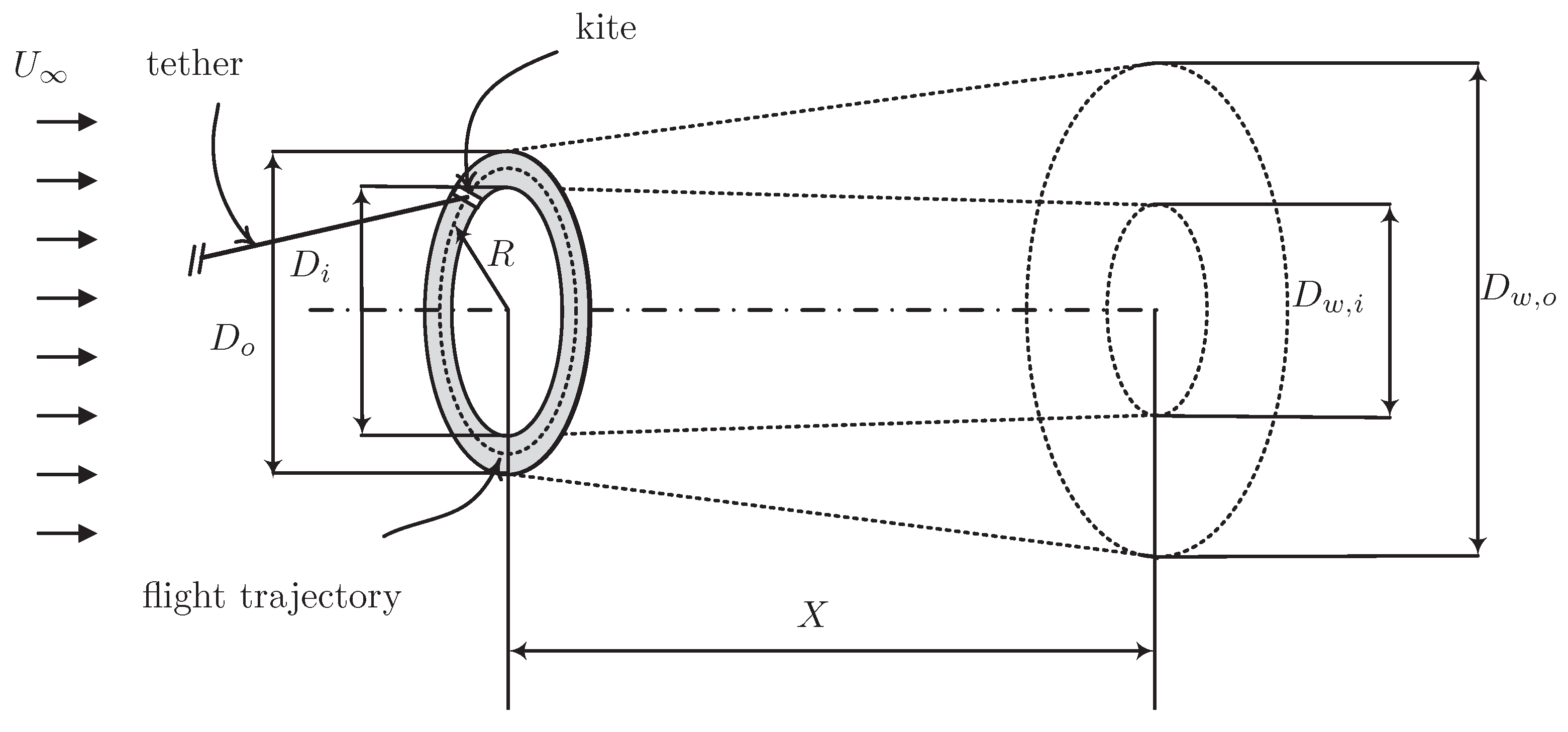
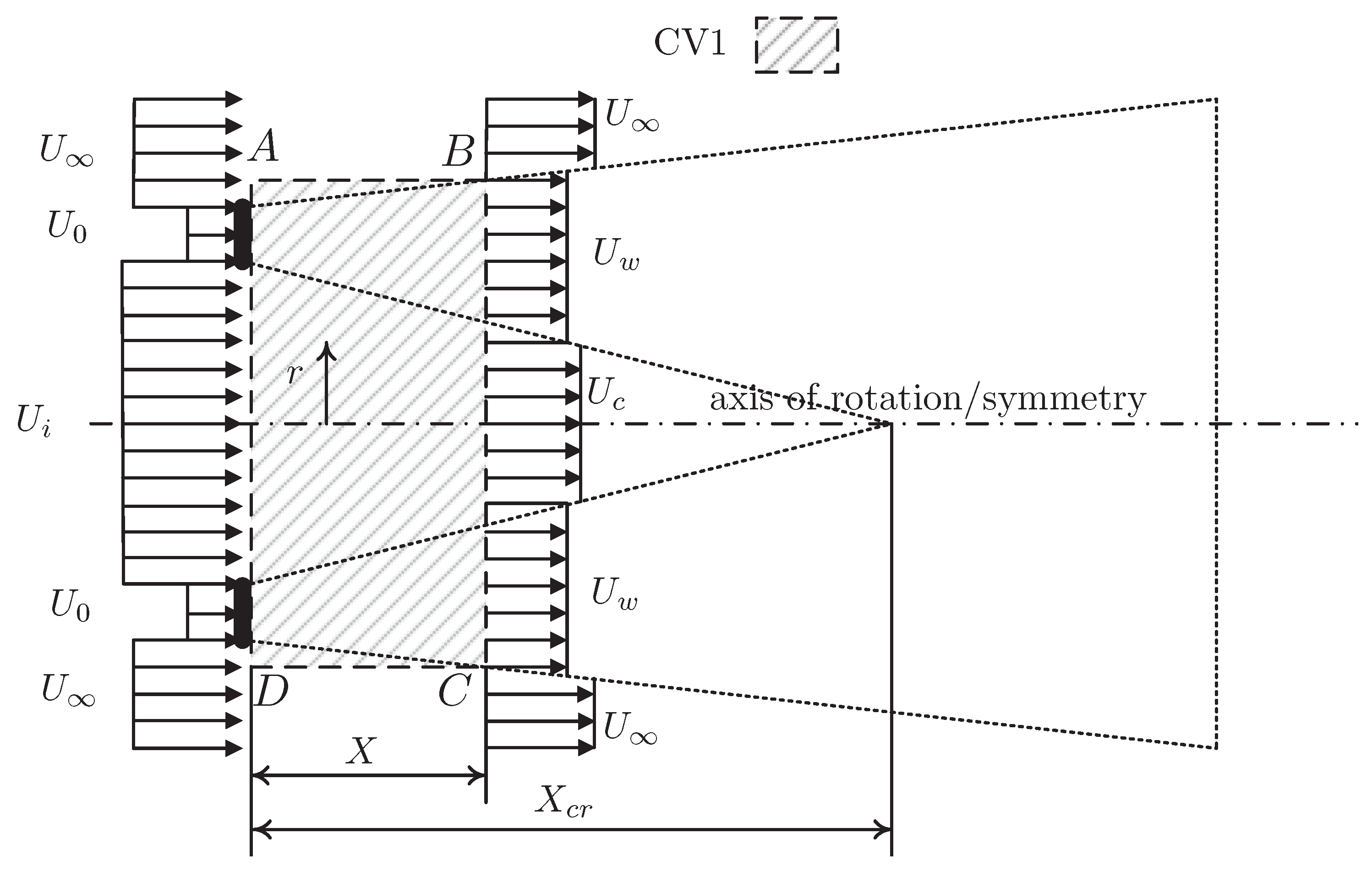
2.1. Theoretical Background

Turbulent flow is characterized by random fluctuations created by the presence of numerous eddies. The increase in turbulence has important effects on the fluid flow parameters, such as density, pressure, and velocity. In general, there are three different methods for turbulent flow calculations: (1) Reynolds-averaged Navier Stokes (RANS) equations ‘closed’ by a turbulence model, (2) large-eddy simulation (LES), and (3) direct numerical simulation (DNS). In the present paper, three-dimensional (3-D), incompressible, unsteady, Reynolds-averaged Navier-Stokes (URANS) equations are solved computationally [33,34]:

$$\begin{array}{c}\frac{\partial u_i}{\partial x_i}=0,\hfill \end{array}$$

(1)

$$\begin{array}{c}\frac{\partial u_i}{\partial t}+u_j\frac{\partial u_i}{\partial x_j}=-\frac{1}{\rho }\frac{\partial p}{\partial x_i}+\frac{\partial }{\partial x_j}(2\nu S_{ij}+{\tau }_{ij}),\hfill \end{array}$$

(2)

where $u_i(i=1,2,3)$ are the mean (or time-averaged) flow velocity components; $\rho$ and p are the density and time-averaged pressure, respectively; $\nu$ is the kinematic viscosity; also, $S_{ij}=(1/2)(\partial u_i/\partial x_j+\partial u_j/\partial x_i)$ are the mean rate of strain tensor (alternatively, $\mu S_{ij}$ are the Newtonian or laminar stresses; $\mu$ being the dynamic viscosity), and ${\tau }_{ij}=-\overline{\rho u_i^{\prime }{u}_j^{\prime }}$ are called Reynolds or turbulent stresses; $u_i^{\prime }$ being fluctuating velocity components; $x_i$ and t are physical coordinates and time, respectively; finally, the overbar indicates the mean value of a quantity, which has been dropped from $u_i$ and p, for convenience.

Here, Menter’s [35] shear-stress transport (SST) turbulence model, commonly referred to as the $k-\omega$ SST turbulence model, is adopted. This means that two additional partial differential equations should be solved simultaneously with Equations (1) and (2):

$$\begin{array}{cc}\hfill \frac{\partial }{\partial t}\left(\rho k\right)+\frac{\partial }{\partial x_i}\left(\rho k{u}_i\right)& =\frac{\partial }{\partial x_j}\left({\Gamma }_k\frac{\partial k}{\partial x_j}\right)+{\tilde{G}}_k-Y_k+S_k,\hfill \end{array}$$

(3)

$$\begin{array}{cc}\hfill \frac{\partial }{\partial t}\left(\rho \omega \right)+\frac{\partial }{\partial x_i}\left(\rho \omega u_i\right)& =\frac{\partial }{\partial x_j}\left({\Gamma }_{\omega }\frac{\partial \omega }{\partial x_j}\right)+G_{\omega }-Y_{\omega }+D_{\omega }+S_{\omega },\hfill \end{array}$$

(4)

$$\begin{array}{cc}\hfill {\Gamma }_k& =\mu +\frac{{\mu }_t}{{\rho }_k},\hfill \end{array}$$

(5)

$$\begin{array}{cc}\hfill {\Gamma }_{\omega }& =\mu +\frac{{\mu }_t}{{\rho }_{\omega }},\hfill \end{array}$$

(6)

where the first equation accounts for the turbulent mixing energy, i.e., the k-equation, and the second governs the specific turbulent dissipation rate, i.e., the $\omega$-equation [36].

In the above equations, ${\rho }_k$ and ${\rho }_{\omega }$ are the turbulent Prandtl numbers for k and $\omega$ and are calculated using blending functions; ${\mu }_t$ is the turbulent viscosity; ${\tilde{G}}_k$ is the generation of turbulent kinetic energy due to mean velocity gradients. Also, $G_{\omega }$ represents the generation of $\omega$, which is calculated as in the $k-\omega$ model of Wilcox [37] (or the standard $k-\omega$ model); ${\Gamma }_k$ and ${\Gamma }_{\omega }$ represent the effective diffusivity of k and $\omega$, respectively, and $D_{\omega }$ is the cross-diffusion term. Lastly, $S_k$ and $S_{\omega }$ are the defined source terms given by the user. For more detailed explanation on the terms, please refer to the user guide of ANSYS Fluent [36].

The SST model utilizes the modified form of the original $k-\omega$ model of Wilcox [37]—by accounting for the effect of the transport of the principal turbulent shear stress ${\tau }_{ij}$—in the inner region of the boundary layer, and it switches to the standard $k-\epsilon$ model away from the wall boundaries (i.e., the outer region) and in free shear flows. The $k-\omega$ SST turbulence model is particularly superior in the prediction of adverse pressure gradient flows often encountered over the blades of wind turbines. To date, many researchers have adopted the $k-\omega$ SST turbulence model for CFD simulations of the flow around wind turbines: refs. [38,39,40,41,42,43] for horizontal-axis wind turbines, and refs. [44,45] for vertical-axis wind turbines, just to name a few.

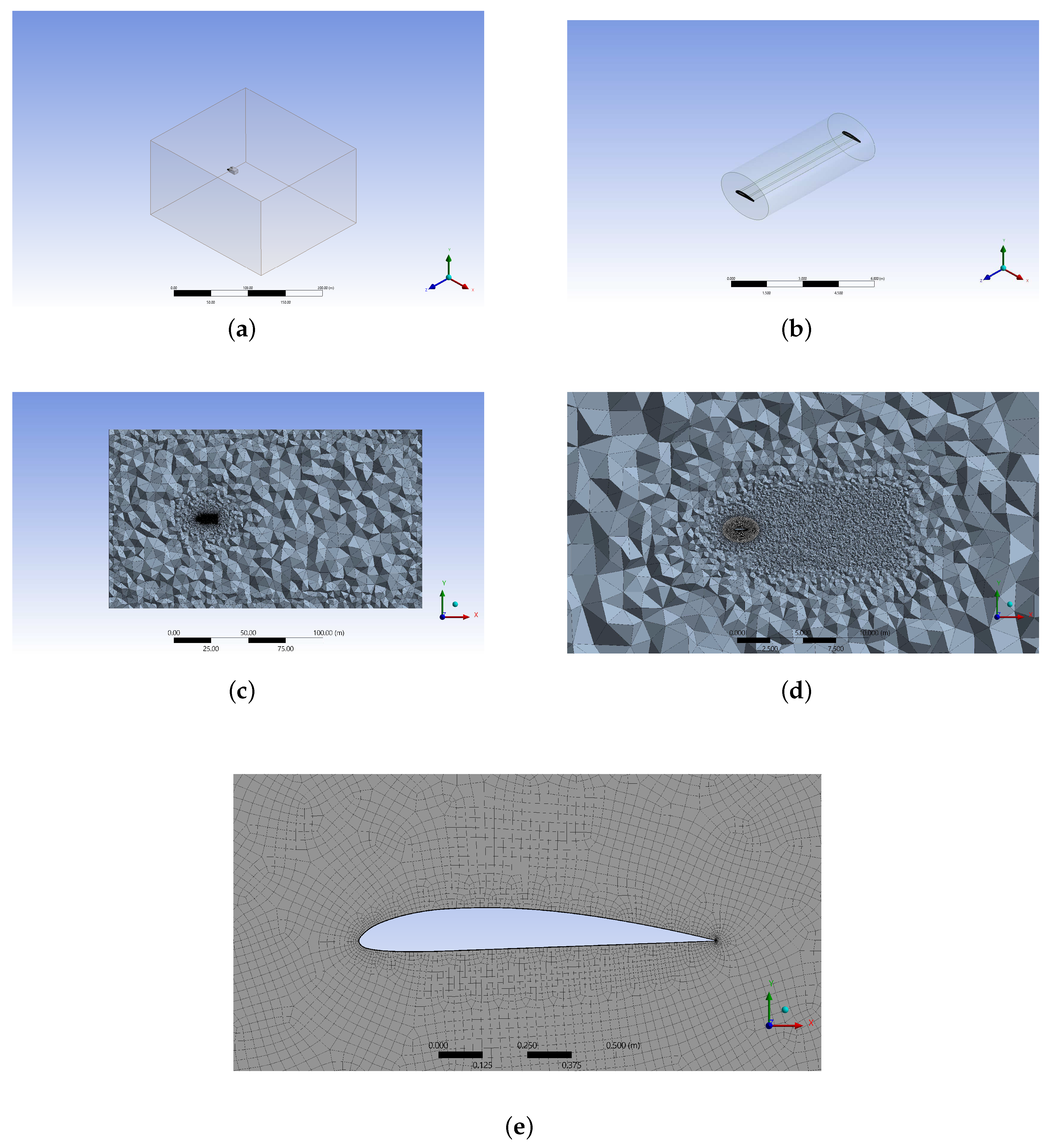
2.2. CFD Simulation Set-Up

Figure 2 shows the CFD solution domain. The distance between the inlet and the outlet, i.e., the length of the simulation domain, is 20 km, and the width and the height of the domain are identical and equal to 9 km. The kite geometry is fully modelled, which is essentially a rectangular wing of span $b=53.94$ m, chord length $c=3.72$ m (aspect ratio $AR=14.5$), and Clark Y airfoil sections. The Clark Y airfoil section was chosen in this study due to its popularity in general aviation and in the field of aerodynamics. Clark Y’s relatively high lift-to-drag ratio, gentle stall, and nearly flat bottom make it very attractive in terms of aerodynamics and construction.

The inlet of the simulation domain is placed 4.5 km upstream of the rotor plane. The reasonably large size of the computational domain, especially the large distance between the rotor plane and the outlet, prevents possible interactions between the wake flow and boundaries and thus ensures the reliability of the flow simulation results. Small downstream distances sometimes lead to solution divergence and sometimes to an overestimate of the power output coefficient. The flow blockage ratio in the solution domain, i.e., the solid area divided by the flow area, is calculated as 0.052%, that is negligible. A uniform spatio-temporal flow velocity of $U_{\infty }=8.33$ m/s with a turbulence intensity of 1% is imposed at the inlet—the velocity inlet condition. The turbulence intensity is commonly defined as the ratio between the root mean square of turbulent velocity fluctuations to the mean flow velocity [33]. The rest of the boundary conditions are: zero gauge pressure at the outlet (i.e., pressure outlet), symmetry over the top, bottom and sides of the domain, and no-slip over all the faces of the kite; see Figure 2a). The SIMPLE algorithm is used for pressure-velocity coupling. Second order upwind scheme is utilized for spatial discretization of the momentum, turbulent kinetic energy, and specific dissipation rate equations. First order implicit scheme is used for time discretization of the transient term.

The nominal power output of the kite is approximately 5.5 MW, which is calculated based on Loyd’s [1] equations for a lift mode CKPS flying at the average altitude of 355 m where the freestream density is ${\rho }_{\infty }=1.1752$ kg/m${}^3$. The kite is flying continuously on a circular path of radius $R=123.3$ m with the angular velocity $\Omega =0.738$ rad/s which corresponds to a linear velocity $V_c=91.03$ m/s. Therefore, the kite sweeps an annular area with the inner diameter $D_i=2R-b=192.66$ m and outer diameter $D_o=2R+b=300.54$ m. It is assumed that the actual kite is tethered and is subjected to a 12.5 m/s wind normal to the swept area. This corresponds to a wind speed in wind power class 7 (following the National Renewable Energy Laboratory’s classification) at 10 m and assuming $\alpha =1/7$ in the power law velocity profile. The kite is reeling-out at one-third of the wind speed (to reach maximum power output according to Loyd’s formulation), so that the relative velocity (i.e., $v_{rel}=(1-1/3)\times 12.5=8.33$ m/s) becomes exactly the same as the inlet flow velocity considered in the CFD simulations. It is further assumed that the kite would fly such that the aerodynamic efficiency, defined as $\chi =C_L{(C_L/C_D)}^2$ [6], reaches the optimal value of $\chi =1.23\times {(1.23/0.1074)}^2=161.3$ and that there is no induction. The optimal value of $\chi$ may be calculated using tables for the lift and drag coefficients of Clark Y airfoil section versus angle of attack (with the Reynolds number of $Re\approx 20\times {10}^6$), which have been corrected for the effects of a finite aspect ratio; see ([46], Chapter 5). It should be noted that $C_D=0.1074$ also includes the effective drag coefficient due to the tether [47].

ANSYS workbench meshing tool [48] is used for mesh generation, and the simulation domain is divided into stationary and rotating domains to allow for the implementation of the sliding mesh method (SMM). The SMM is a special case of dynamic mesh motion, where nodes move rigidly, provided that cell zones are connected through non-conformal interfaces. The kite is placed in the middle of the rotating domain, which rotates counterclockwise; see Figure 2b). Wake flow analysis requires a smooth, uniform mesh growth rate; therefore, the patch independent method is used to create the transitional mesh between the rotating and stationary domains. This method provides additional control over the maximum element size and leads to a smooth transition of the mesh. The maximum element size of the rotating domain is at the interface. A sphere of influence (of radius of 640 m) is created in the downstream region of the kite to effectively capture the physics of the wake flow; see Figure 2c,d. The advanced size function is also enabled with refinement options set to proximity and curvature – this helps to adequately capture and mesh small edges of an airfoil. The global and local mesh controls options are utilized to dictate the mesh refinements regions, faces and edges. In the solution domain, in total, there are 6.9 million cells and 3.8 million nodes. The maximum mesh skewness is 0.83.

The upper and lower sides of the airfoil are split in half to apply different mesh densities with more concentrations towards the leading and trailing edges. A bias factor of 2 is applied towards the leading edge while it is 10 towards the trailing edge. 22 inflation layers are created around the kite geometry to reliably simulate flow in the boundary layer and to accurately capture flow separation; see Figure 2e). The first layer height is defined by the $y^{+}$ requirements (i.e., $y^{+}\sim 1$) with a steady growth rate of 1.2. The airfoil mesh is swept across the kite surface to ensure better mesh quality and uniform inflation layers. The total number of hexahederal elements that are swept across the kite surface is around 3 millions.

The CFD simulation is performed using ANSYS Fluent, which employs a finite volume method for solving the Navier-Stokes equations, on Compute Canada clusters (accessed 12 cores and 192 GB of RAM). For the present study, the transient flow analysis is adopted. As mentioned earlier, the sliding mesh method is employed to model the transient flow effects between the stationary and rotating domains. The rotational velocity of the rotating domain is set at the angular velocity of the kite. The solution time step was considered to be equivalent to $\Delta \theta =1$ deg of rotation (i.e., $\Delta t=\Delta \theta /\Omega =$ 0.0236 s, CFL number = 0.43). This time step was judged to be sufficiently small considering best practices adopted for CFD simulation of similar systems, such as H-type Darrieus [44], and Savonius [49] wind turbines. The simulation was ran up to 51 cycles (each cycle took almost 24 h CPU time) to ensure the wake flow is fully developed up to large distances (i.e., $12R$) from the rotor. Two criteria were established to ensure the solution is converged and reached post-transient conditions. The first criterion is that the residual values should fall below ${10}^{-5}$. The second criterion is met by monitoring the average value of the axial flow velocity over multiple concentric annuli across the wake width at several points from the rotor (e.g., at $x=5R$ and $x=8R$). The solution is assumed to have converged when for any two successive revolutions of the kite, the average difference between the velocities at equivalent time steps within the period is less than 1%.

The methodology used in the CFD simulation of the kite, which was discussed above, is verified by considering computational results from two other simulations performed for an airfoil (Appendix A) and for a wing (Appendix B). This may be an acceptable verification approach given the lack of experimental data on the aerodynamics of crosswind kites. Although some flow features in the kite simulation, such as wake rotation, is absent from the airfoil/wing simulations, still, these two simulations and the kite simulation share some common flow features, such as boundary layer development, tip vortices generation, and possible flow separation. A similar simulation setup and mesh setting as those mentioned above have been used in the airfoil/wing simulations, and, wherever possible, a similar geometry and flow Reynolds number have been adopted; please see Appendix A and Appendix B for more details.

2.3. Results and Discussion

2.3.1. Induction Factor

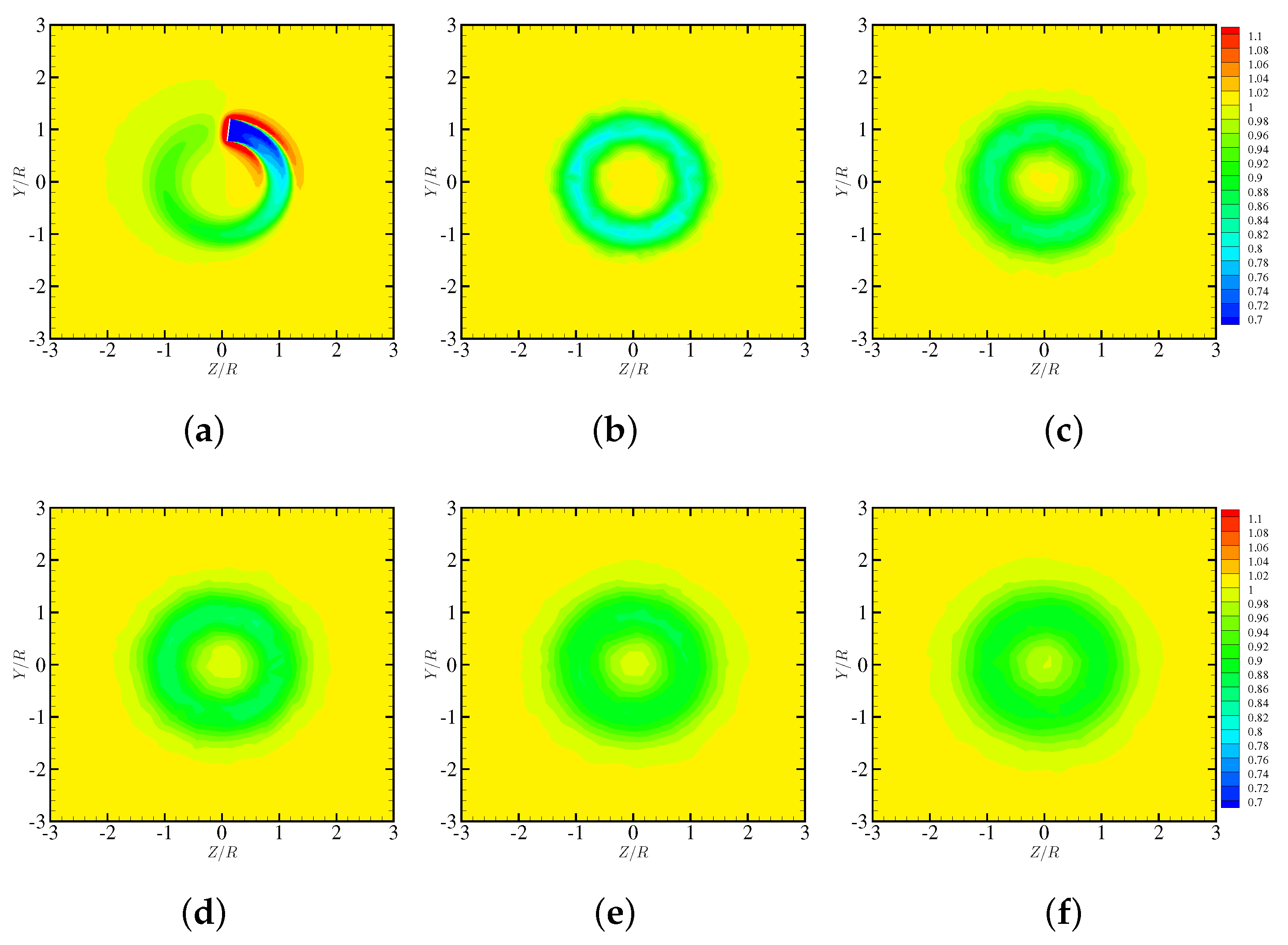
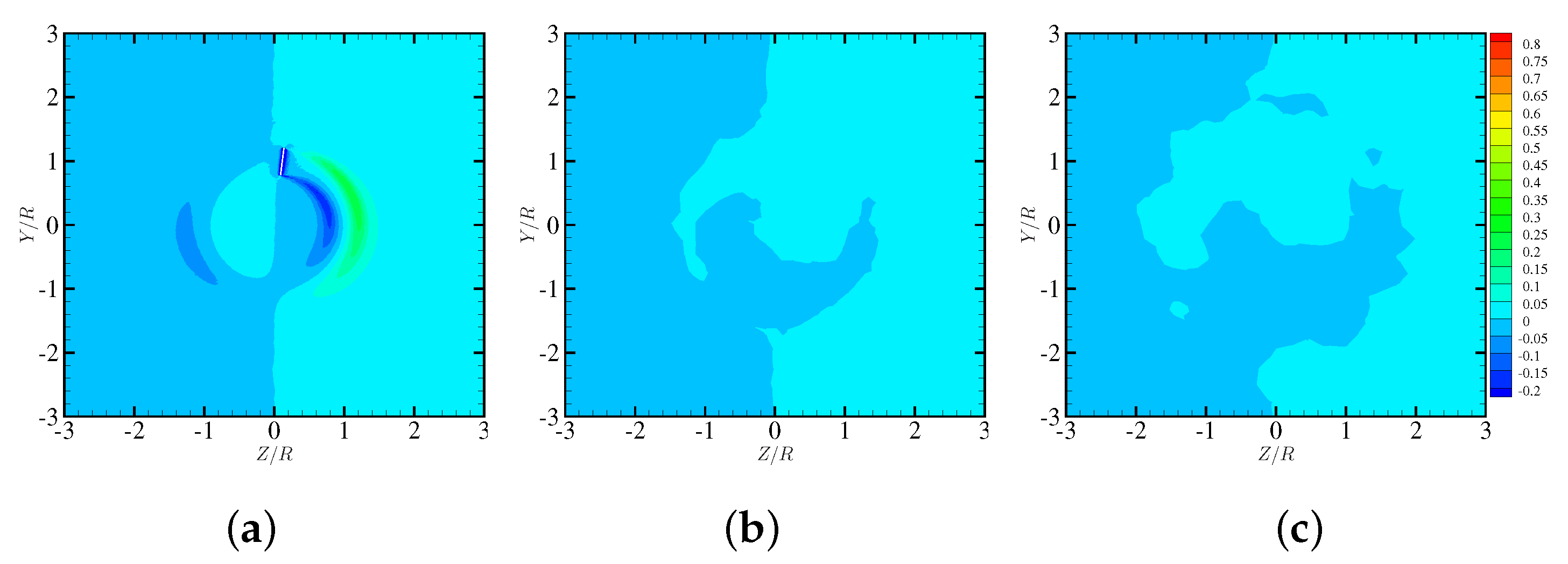
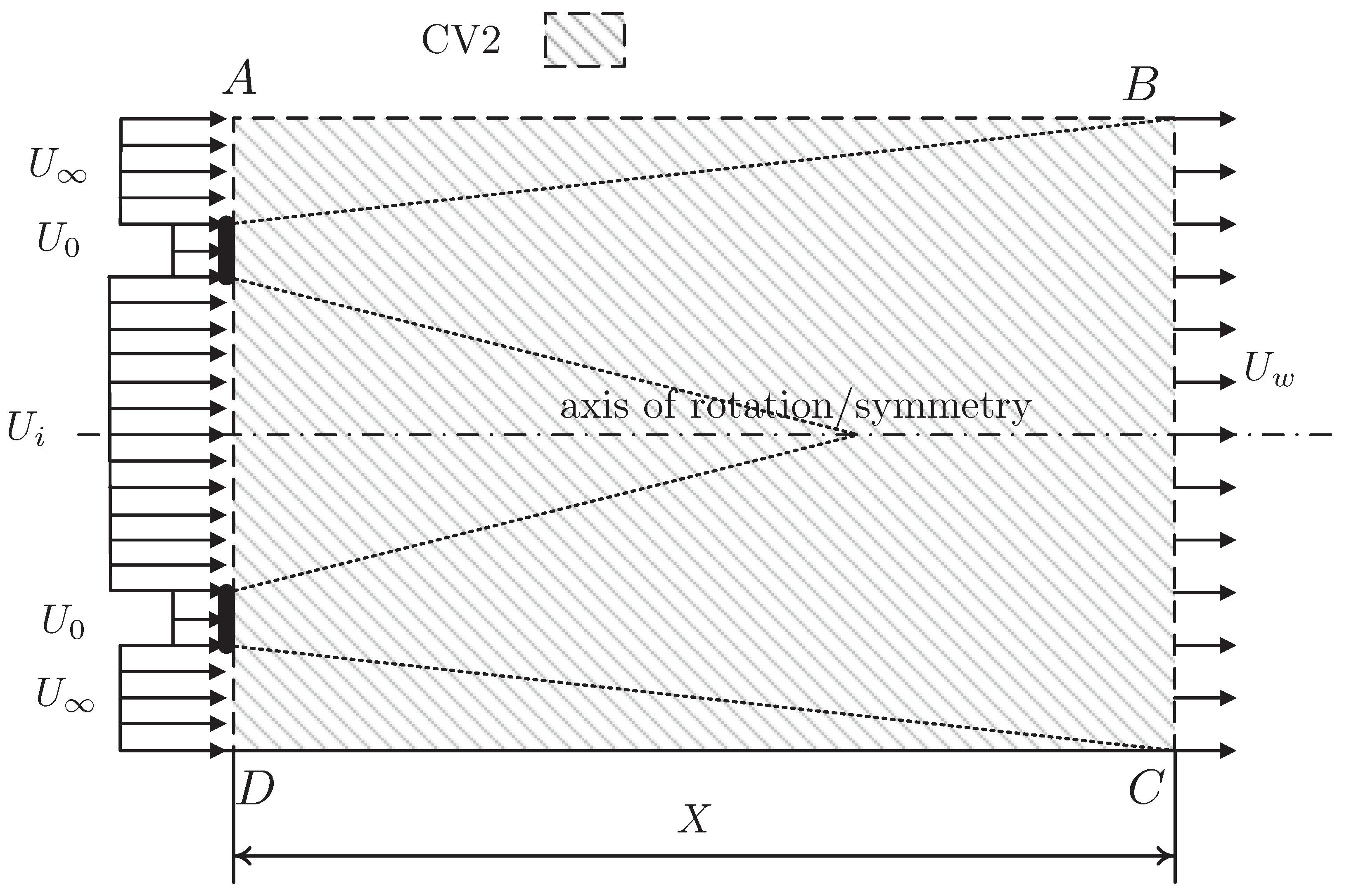
According to the axial momentum theory [39,50,51], flow undergoes a velocity reduction and a simultaneous pressure increase when approaching an energy extracting device, such as a wind turbine or a crosswind kite. The magnitude of flow velocity reduction at the turbine/kite is commonly expressed as $a{U}_{\infty }$. In general, the axial (or streamwise) induction factor a may be defined as the ratio between the axial flow velocity induced by an energy extracting/generating device and the freestream velocity, $U_{\infty }$. In other words, a may be defined as $a=1-(U/U_{\infty })$, where U is the flow velocity component normal to the plane of rotation at any point on that plane. The acceptable range of the mean value of a for a wind turbine or a crosswind kite is $0<a<1/2$ while for an energy generating device, such as a propeller, $a<0$. The induction factor can be linked to the power coefficient of the device, which for a wind turbine-like device can reach at best $16/27\approx 59.3\%$ (known as the Betz-Joukowsky limit [52]) which occurs when $a=1/3$. When the flow passes through an energy extracting device, the static pressure undergoes a sudden reduction while the flow velocity remains almost unchanged.

Figure 3 shows the contour plots of the instantaneous axial induction factor at the kite location while the kite flies counterclockwise on a circular path. The kite is shown as a white rectangle in the figure. More precisely, the white region is the pressure side of the kite, which is subjected to the incoming wind flow. In the figure, positive values (i.e., warm colours) indicate flow retardation, while negative values (i.e., cool colours) indicate flow acceleration. Induction values higher than 1 may indicate a reverse flow which can occur close to the kite tips. At the tips, the axial velocity ‘induced’ by tip vortices is typically larger than that at in-board points. From Figure 3, flow retardation in the wake of the kite and acceleration in the regions close to the front and sides of the kite as well as in the inner (or core) region of the annulus swept by the kite are evident. The inner region may be defined as the area between the axis of rotation and the innermost tip of the kite. It is also evident that a greater flow retardation occurs close to the kite trailing edge, which gradually diminishes at larger distances from the kite on the circular path. This appears reasonable since during the time that the kite is advancing in a cycle, the regions already swept by the kite will be exposed to fresh undisturbed flow and thus be recovering from the effects of the presence of the kite.

Following the ‘reduced axial velocity method’ [53,54], which was originally developed for conventional wind turbines, the flow area is divided into multiple concentric rings (or annuli) over which the axial flow velocity is averaged. From the above equation for a, the average induction factor over each ring is obtained, where $a_{r,i}$ being the average induction over the ith ring; $a_{r,i}$ may be considered to be effectively acting at a radial distance corresponding to the center of the ring. Thus, one can obtain a radial distribution of the average induction factor, i.e., $a_r\left(r\right)$, which for the kite in the present study is shown in Figure 4. On the other hand, the global induction factor, $\overline{a}$, is obtained by averaging the radial induction values: $\overline{a}={\sum }_{i=1}^n{w}_i{a}_{r,i}$, where $w_i=A_{r,i}/A_s$ is the ratio between the ith ring area and the total area swept by the kite. This global induction factor is an indicator of the overall aerodynamic performance of the kite. For the kite whose radial distribution of the average induction factor is shown in Figure 4, the global induction factor is calculated as $\overline{a}=0.127$ which is in good agreement (≈0.6–6% relative error) with the values obtained analytically [11,47] for the same kite. It should be noted that in ref. [11] the arithmetic mean of induction values over the rings covering the swept area was reported as the CFD-calculated induction factor. It is also interesting to note that $\overline{a}$ obtained computationally using a URANS flow solver closed by the $k-\epsilon$ turbulence model is only different by less than $2\%$ from that obtained here by employing the $k-\omega$ SST turbulence model; refer to [11] for more details.

2.4. Wake Flow

Figure 5 shows the distribution of the instantaneous static pressure coefficient, $C_p$, and the dimensionless axial (or X-component) flow velocity, $U/U_{\infty }$, in the $YZ$-plane ($6R\times 6R$ in size) at different dimensionless axial distances $X/R=0.25,0.50,0.75,\mathrm{and}1$, from the plane of rotation. The static pressure coefficient is defined as $C_p=(p-p_{\infty })/(1/2{\rho }_{\infty }{U}_{\infty }^2)$, where p and $p_{\infty }$ are the local and freestream static pressures, respectively. Typically, when the flow passes through an energy extracting device, the static pressure undergoes a sudden drop. As the wake flow moves downstream, it expands, where the static pressure increases and reaches the ambient pressure while the flow velocity inside the wake decreases. This marks the end of the initial expansion region, the length of which for conventional wind turbines is estimated to be about one diameter [28]. Nevertheless, some researchers, such as Frandsen et al. [23] and Bastankhah and Porte-Angel [24] argued that it is difficult to exactly determine the length of this region.

As discussed in [28] and also confirmed by the plots shown in Figure 5, the regions immediately downstream the rotation plane are featured by non-uniform pressure and axial flow velocity deficit (i.e., $C_p<0$, $U/U_{\infty }<1$). As seen, by increasing the axial distance from $X/R=0.25$ to 1, $C_p$ vanishes increasingly over the flow area. It is evident that the static pressure gradually increases by $X/R$ and eventually reaches the ambient static pressure at $X/R=1$ or soon after. The static pressure increase is accompanied by a flow velocity reduction as may be confirmed from Figure 5e–h. Thus, one may take $X=R$ as the end of the initial expansion region for the present crosswind kite. Nevertheless, it is too early to generalize this observation for other kite systems. Additional CFD simulations for kites of different scales, and more favourably, experimental studies are required to reach a general conclusion.

Figure 6 shows the distribution of the instantaneous, dimensionless axial flow velocity, $U/U_{\infty }$, in the $YZ$-plane at $X/R=0,2,4,6,8,\mathrm{and}10$. These plots were obtained after the kite completed 50 cycles of rotation. At $X/R=0$, as seen from Figure 6a, the flow velocity distribution in the $YZ$-plane is asymmetric, obviously due to the presence of the kite. Moreover, as also discussed in Section 2.3.1, flow acceleration (i.e., $U/U_{\infty }>1$) can be observed in the front and sides of the kite. As seen from Figure 6b–f, as the wake moves further downstream, the axial flow velocity becomes nearly axisymmetric. Also, the annular wake flow becomes thicker as $X/R$ is increased, which means that the wake expands towards both inner and outer undisturbed flows.

Figure 7 and Figure 8 show the distribution of the instantaneous dimensionless flow velocity in the vertical (or Y-axis) and lateral (or Z-axis) directions, represented by $V/U_{\infty }$ and $W/U_{\infty }$, respectively. At $X/R=0$, as seen from Figure 7a, in the inner flow region and for $Y>0$, $V/U_{\infty }$ has a predominantly negative sign while it is primarily positive for $Y<0$, indicating that the flow is convergent in that region. On the other hand, in the outer region, the flow is generally divergent (or expanding), where the kite pushes the flow up in the positive half-plane and thus $V/U_{\infty }>0$ while it pushes down the flow in the negative half-plane and thus $V/U_{\infty }<0$. In Figure 7b,c, arrows (which represent the in-plane flow velocity vector) confirm the flow expansion but also show that the expansion is diminished as $X/R$ is increased. Moreover, it is observed that the wake rotates in the clockwise direction as it moves downstream. This makes perfect sense since the kite spins in the counterclockwise direction. As a result, a flow asymmetry appears in the inner flow region and area swept by the kite, where $V/U_{\infty }>0$ and $V/U_{\infty }<0$ on most parts of the left and right semicircles (of the radius of approximately R), respectively. Similar observations can be made from plots shown in Figure 8, which are not repeated here for the sake of brevity.

3. A Simple Analytical Wake Model

In Section 2.4, the length of the initial wake expansion region for the present study crosswind kite system was obtained computationally to be about R. Nevertheless, for simplicity and inspired by the work of [20,21,23], it is assumed that the initial expansion behind the kite occurs immediately; in other words, the initial expansion region has a negligible length (Assumption 1). From the momentum theory, the axial flow velocity where the initial expansion region ends, is obtained from [39,50,51]:

$$U_0=U_{\infty }(1-2a).$$

(7)

Figure 9 shows schematically the annular wake (dotted line) downstream of a crosswind kite in the straight downwind configuration, where the kite flies essentially on a plane (referred to as rotation plane) normal to the incoming wind which is considered to be steady and uniformly distributed (Assumption 2). The fact that a crosswind kite sweeps an annulus in the sky permits considering an annular wake flow. It should be noted that this is the wake developed past the initial expansion region. Considering Assumption 1, one may then conclude that the wake essentially starts developing immediately after the rotation plane, as shown in Figure 9. It is assumed that the wake flow is entirely axial (i.e., with no rotational motion) and axisymmetric and that it expands linearly as a function of the axial coordinate X (Assumption 3). Motivated by the assumption made in [20,21] for wind turbines, it is further assumed that the wake has a starting width equal to the width of the annulus swept by the kite (Assumption 4); that is, $D_{w,i}(X=0)=D_i$ and $D_{w,o}(X=0)=D_o$, where $D_{w,i}$ and $D_{w,o}$ are the inner and outer diameters of the wake, respectively; see Section 2.2 for the definition of $D_i$ and $D_o$. The wake radius expansion is assumed to occur at two different rates towards the outer and inner flow regions, which are represented by ${\kappa }_o$ and ${\kappa }_i$, respectively (Assumption 5). The rate of wake expansion, the so-called “entrainment” or “decay” constant, for on-shore conventional wind turbines is typically taken between 0.05 and 0.1 [20,23,24]. A commonly-used semi-empirical equation for estimating the entrainment constant for wind turbines is $\kappa =0.5/ln(h/z_0)$, where h is the hub height, and $z_0$ is the surface roughness length [55].

See Figure 10 which shows a section of the wake flow (dotted line) downstream of a crosswind kite and that of the control volume CV1 (hatch pattern) enclosing a flow region downstream the rotation plane. The boundaries of CV1 are specified by $ABCDA$; the inlet $AD$ is located where the initial expansion ends (marked by $X=0$), which is immediately after the rotation plane (see Assumption 1). The outlet, on the other hand, is placed upstream of the critical point, i.e., $X<X_{cr}$. The critical point (marked by $X_{cr}$) is defined as the point where the wake inner diameter vanishes. The side boundaries $AB$ and $CD$ are parallel to the freestream. At the inlet, as seen from the figure, the velocity of the flow going into CV1 along radial range $0\le r<(D_i/2)$ is uniform and of magnitude $U_i$. The flow velocity along $(D_i/2)<r<(D_o/2)$ is $U_0$ (see Equation (7)), and that is $U_{\infty }$ for $(D_o/2)<r<(D_{w,o}/2)$.

The flow velocity inside the wake at any point along the X-axis is considered uniform. This is equivalent to the so-called “top-hat” distribution of the velocity deficit in the wake, which is used for simplicity, in contrast to a more accurate but also more complex Gaussian or bell-shaped distribution (see, e.g., ref. [24] which considers the Gaussian velocity profile for conventional wind turbines). Moreover, the uniform distribution automatically satisfies “self-similarity” of wake flow velocity often assumed in the analytical wake models for conventional wind turbines. Thus, at the outlet $BC$, the velocity of the flow leaving CV1 along the radial range of $(D_{w,i}/2)<r<(D_{w,o}/2)$ is uniform and is denoted by $U_w$. Moreover, the flow velocity within the inner region $0\le r<(D_{w,i}/2)$ is assumed uniform and is denoted by $U_c$. No inflow or outflow occurs across $AB$ and $CD$ since they are, in fact, streamlines which are parallel to the freestream.

Considering the control volume CV1, the equation for the conservation of mass may be written as:

$$\frac{\pi }{4}{D}_i^2{U}_i+\frac{\pi }{4}(D_o^2-D_i^2)U_0+\frac{\pi }{4}(D_{w,o}^2-D_o^2)U_{\infty }=\frac{\pi }{4}{D}_{w,i}^2{U}_c+\frac{\pi }{4}(D_{w,o}^2-D_{w,i}^2)U_w.$$

(8)

Using the assumption that the wake expands linearly with the axial distance X from the rotation plane, we can write

$$D_{w,o}=D_o+2{\kappa }_{o}X,D_{w,i}=D_i-2{\kappa }_{i}X,$$

(9)

where $2{\kappa }_o$ and $2{\kappa }_i$ are the rates at which the wake diameter expands towards the freestream and the axis of rotation, respectively.

From Equations (8) and (9), one can obtain

$$\begin{array}{cc}\hfill D_i^2{U}_i+(D_o^2-D_i^2)U_0& +[{(D_o+2{\kappa }_{o}X)}^2-D_o^2]U_{\infty }\hfill \\ \hfill ={(D_i-2{\kappa }_{i}X)}^2{U}_c& +[{(D_o+2{\kappa }_{o}X)}^2-{(D_i-2{\kappa }_{i}X)}^2]U_w,\hfill \end{array}$$

(10)

which by defining ${\delta }_i=D_i/2R$, ${\delta }_o=D_o/2R$, $\xi =X/R$, ${\upsilon }_0=U_0/U_{\infty }$, ${\upsilon }_i=U_i/U_{\infty }$, ${\upsilon }_c=U_c/U_{\infty }$ and ${\upsilon }_w=U_w/U_{\infty }$ is further simplified to

$${\upsilon }_w={\displaystyle \frac{{\delta }_i^2{\upsilon }_i+({\delta }_o^2-{\delta }_i^2){\upsilon }_0+{({\delta }_o+{\kappa }_o\xi )}^2-{\delta }_o^2-{({\delta }_i-{\kappa }_i\xi )}^2{\upsilon }_c}{{({\delta }_o+{\kappa }_o\xi )}^2-{({\delta }_i-{\kappa }_i\xi )}^2}}.$$

(11)

Using the control volume CV2 shown in Figure 11, the dimensionless wake velocity for $X>X_{cr}$ (or alternatively $\xi >{\xi }_{cr}$) is obtained as

$${\upsilon }_w={\displaystyle \frac{{\delta }_i^2{\upsilon }_i+({\delta }_o^2-{\delta }_i^2){\upsilon }_0+{({\delta }_o+{\kappa }_o\xi )}^2-{\delta }_o^2}{{({\delta }_o+{\kappa }_o\xi )}^2}},$$

(12)

and the dimensionless counterpart of Equation (9) can be written as

$${\delta }_{w,o}={\delta }_o+{\kappa }_o\xi ,{\delta }_{w,i}={\delta }_i-{\kappa }_i\xi .$$

(13)

A simplifying assumption is to consider the flow velocity in the inner region to remain constant and equal to the freestream velocity, i.e., ${\upsilon }_i={\upsilon }_c=1$; a similar assumption was made in [31]. From CFD results presented in Section 2.4, it is seen that ${\upsilon }_c$ may actually reach values above 1, which means that flow may accelerate inside the inner region; nevertheless, this increase of flow velocity is minimal and still the assumption of ${\upsilon }_c=1$ may be reasonable. Moreover, from Equation (7), ${\upsilon }_0=1-2a$; thus, Equations (11) and (12) may be simplified to

$${\upsilon }_w=1-{\displaystyle \frac{2a({\delta }_o^2-{\delta }_i^2)}{{({\delta }_o+{\kappa }_o\xi )}^2-{({\delta }_i-{\kappa }_i\xi )}^2}},$$

(14)

and

$${\upsilon }_w=1-{\displaystyle \frac{2a({\delta }_o^2-{\delta }_i^2)}{{({\delta }_o+{\kappa }_o\xi )}^2}},$$

(15)

respectively.

Equations (14) and (15) provide simple mathematical equations to obtain the flow velocity in the wake as a function of $\xi$; moreover, with Equation (13) one can calculate the wake size as it expands downstream. Nevertheless, one should note the limitations of the model, the first being the unrealistic assumption of top-hat distribution of the velocity deficit and the second being the fact that the model solely considers the conservation of mass. In fact, one can mathematically show that the present model violates the conservation of momentum law in the wake, and the violation grows with $\xi$ [32]. See Appendix C which provides some expressions to quantify the deviation from the conservation of momentum law.

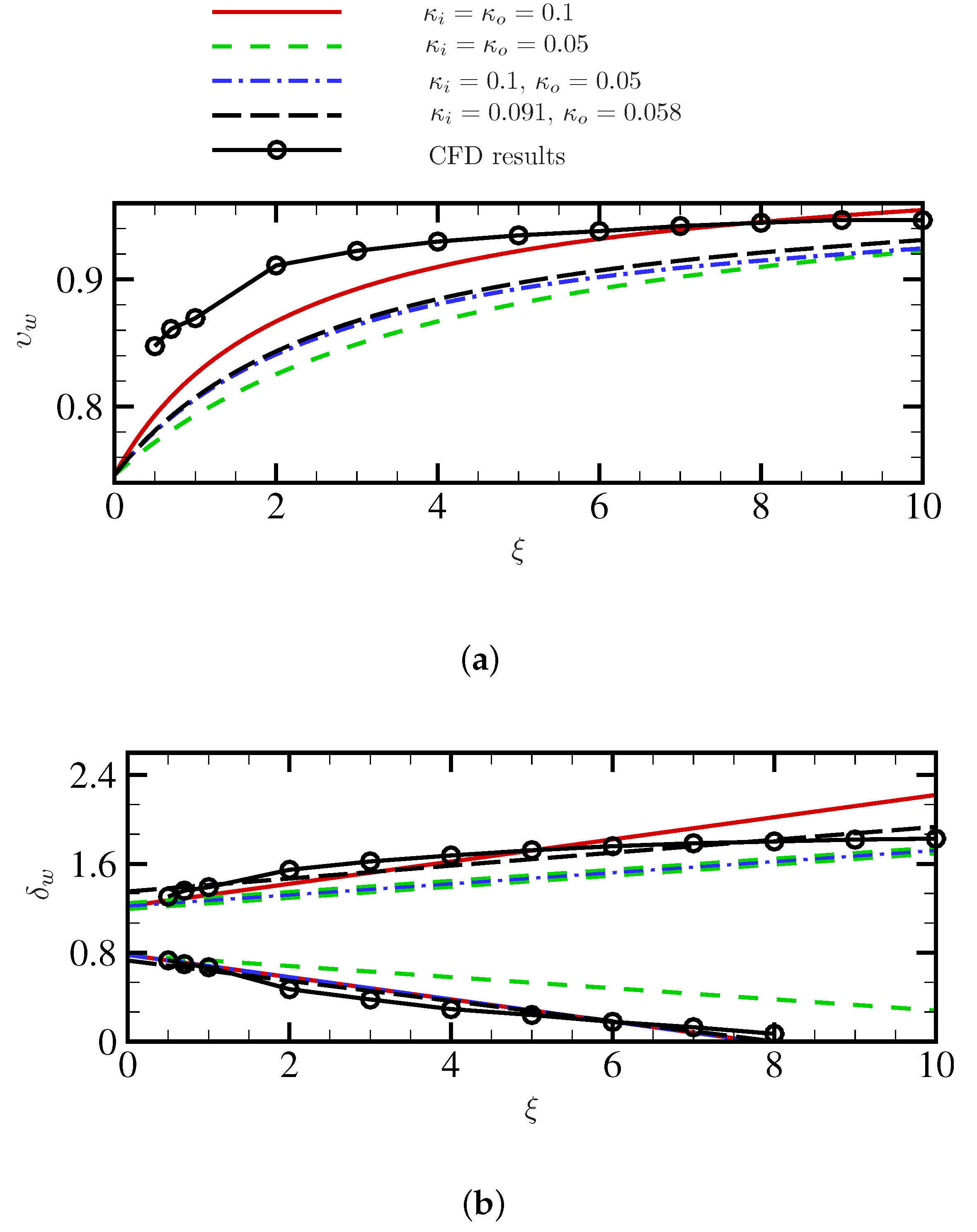
4. Comparison between CFD and Analytical Results

We adopt the method proposed in [27] to obtain the wake radii and the average wake velocity from the CFD results presented in Section 2. The wake boundary (or width) in the radial direction at any streamwise coordinate $\xi$ is considered as the point where the flow velocity reaches 99% of the freestream velocity—Kaufman-Martin et al. [31] considered the surface where the flow velocity reached the freestream velocity as the wake boundary. The average wake velocity was also obtained by integrating the area under the velocity profile between the wake inner and outer radii.

Figure 12 shows the comparison between CFD results (circle markers) and those obtained via the analytical model for four different sets of entrainment constants ${\kappa }_i$ and ${\kappa }_o$: ${\kappa }_i={\kappa }_o=0.1$ (solid line, red online), ${\kappa }_i={\kappa }_o=0.05$ (dashed line, green online), ${\kappa }_i=0.1,{\kappa }_o=0.05$ (dash-dotted line, blue online), and ${\kappa }_i=0.091,{\kappa }_o=0.058$ (long dashed line, black online). Subfigures (a) and (b) show, respectively, the variation of ${\upsilon }_w$ and ${\delta }_w$ (${\delta }_w$ is used to refer to both ${\delta }_{w,o}$ and ${\delta }_{w,i}$) as a function of $\xi$. The first three analytical sets are basically different combinations of 0.1 and 0.05, which are typical entrainment constants used for conventional wind turbines onshore; see Section 3. The last set of ${\kappa }_i$ and ${\kappa }_o$ was found by fitting lines to the CFD wake inner and outer radii curves.

As seen from Figure 12a, the CFD wake velocity recovers quite fast within $\xi \le 2$ with ${\upsilon }_w$ increasing above 0.9, while it almost plateaus at higher values of $\xi$. The analytical model with the given entrainment constants generally underestimates the value of ${\upsilon }_w$. The best agreement is achieved with ${\kappa }_i={\kappa }_o=0.1$ although the curves with other values of ${\kappa }_i$ and ${\kappa }_o$ may lead to a better agreement beyond $\xi =10$ based on their trends. As seen from Figure 12b, according to CFD results, the wake expands almost linearly with $\xi$ but with two different rates within $\xi ⪅2$ and $\xi ⪆2$ wake regions. In addition, the rate of wake expansion is quite different towards the inner and outer flow regions. Considering the quality of agreement over both ${\upsilon }_w$ and ${\delta }_w$, particularly for larger values of $\xi$, all analytical results, except those obtained via ${\kappa }_i={\kappa }_o=0.05$, appear to reasonably match the CFD results. See

Table 1. Comparison between analytical and CFD results, where the mean and standard deviation of the relative difference between the two sets of results are given.

${\mathit{\kappa }}_{\mathit{i}}$, ${\mathit{\kappa }}_{\mathit{o}}$	${\mathit{\upsilon }}_{\mathit{w}}$		${\mathit{\delta }}_{\mathit{w},\mathit{i}}$		${\mathit{\delta }}_{\mathit{w},\mathit{o}}$
	Mean (%)	STD (%)	Mean (%)	STD (%)	Mean (%)	STD (%)
${\kappa }_i={\kappa }_o=0.1$	2.6	2.4	15.5	14.6	7.7	6.2
${\kappa }_i={\kappa }_o=0.05$	6.3	2.6	83.8	80.3	10.9	3.9
${\kappa }_i=0.1$, ${\kappa }_o=0.05$	5.2	2.2	15.5	14.6	10.9	3.9
${\kappa }_i=0.091$, ${\kappa }_o=0.058$	4.8	2.4	13.7	9.5	3.8	1.9

for a quantitative comparison between analytical and CFD results. In the table, the mean and standard deviation of the relative difference between the two sets of results for wake velocity and wake radii have been provided.

Figure 13 shows the wake velocity profile, more precisely, the radial distribution of the time-averaged wake velocity, obtained from the CFD simulation (solid line) and that obtained via the analytical model (dashed line) at different axial distances from the rotation plane for (a) ${\kappa }_i={\kappa }_o=0.1$, and (b) ${\kappa }_i=0.091$, ${\kappa }_o=0.058$. As seen, the CFD velocity profile looks like a Gaussian profile while the analytical one is a top-hat profile as was assumed in the beginning. From CFD profiles, it is evident that the flow velocity in the inner flow region is slightly higher than the freestream velocity (i.e., ${\upsilon }_w>1.0$) for $\xi \le 2$ while it gradually decreases by increasing $\xi$ but remains very close to the freestream velocity.

5. Concluding Remarks

In this paper, using the CFD model, some aspects of the aerodynamics in the vicinity and downstream of a multi-megawatt CKPS were examined. URANS equations closed by the $k-\omega$ SST turbulence model were solved numerically inside a large simulation domain. The radial distribution of the average axial induction factor as well as the global induction factor were obtained by following the reduced axial velocity method. Next, the variation of the static pressure and the axial flow velocity in small axial distances from the rotation plane were obtained. For the kite considered in this study, the initial expansion region was found to extend up to one gyration radius from the rotation plane, which is comparable to that of conventional wind turbines. The wake rotation caused an asymmetry in the vertical and lateral wake flow velocities while the axial flow velocity became increasingly axisymmetric as the axial distance from the rotation plane was increased. Although the flow velocity deficit in the wake reduced as the axial distance was increased, flow velocity deficits as large as 10% could be observed at large distances such as 10 times the gyration radius from the rotation plane. This means potentially a maximum of 27% reduction in the available wind power. CFD models can provide much details about the flow dynamics around kite power systems. However, it is not practical to use such models for, for example, conducting preliminary kite farm studies (where many simulations are normally required) due to their prohibitive CPU time.

In addition, in the present paper, the viability of developing a simple analytical wake model for CKPSs was proved. The present model, and those which will be developed subsequently, will pave the way for a better estimation of energy capture in kite farms and their layout design and optimization. These are crucial for estimating the levelized cost of energy for CKPSs, which directly relates to commercialization prospects of such systems. The model was built based on a similar model, known as Jensen’s model in the literature, for conventional wind turbines. Comparisons between numerical results obtained from the proposed analytical model and those from the CFD simulation showed that the analytical model may be able to provide accurate information regarding the average wake flow velocity and its radii. The simple form of the analytical model permits fast computations, which in turn make the model ideal for conducting preliminary as well as optimization studies. Nevertheless, the level of accuracy of the analytical model appeared to be largely dependent on the magnitude of entrainment constants. Thus, future studies should highlight the correlation between the design parameters of a kite system and the entrainment constants. In the absence of publicly available experimental data, more computational studies, which preferably consider the wind gradient due to atmospheric boundary layer, would be necessary for finding a suitable range and/or closed-form equation for the entrainment constants to be used for CKPSs. Moreover, more rigorous analytical wake models such as those satisfying also the conservation of momentum and those considering a Gaussian-like velocity profile are desirable.

References

1. Loyd, M.L. Crosswind Kite Power. J. Energy (AIAA) 1980, 4, 106–111. [Google Scholar] [CrossRef]
2. Fagiano, L.; Milanese, M. Airborne wind energy: An overview. In Proceedings of the American Control Conference (ACC), Montreal, QC, Canada, 27–29 June 2012; pp. 3132–3143. [Google Scholar]
3. Ahrens, U.; Diehl, M.; Schmehl, R. (Eds.) Airborne Wind Energy; Springer: Berlin, Germany, 2013. [Google Scholar]
4. Cherubini, A.; Papini, A.; Vertechy, R.; Fontana, M. Airborne wind energy systems: A review of the technologies. Renew. Sustain. Energy Rev. 2015, 51, 1461–1476. [Google Scholar] [CrossRef] [Green Version]
5. Schmehl, R. (Ed.) Airborne Wind Energy; Springer: Singapore, 2018. [Google Scholar]
6. Kheiri, M.; Nasrabad, V.S.; Bourgault, F. A new perspective on the aerodynamic performance and power limit of crosswind kite systems. J. Wind. Eng. Ind. Aerodyn. 2019, 190, 190–199. [Google Scholar] [CrossRef]
7. Zanon, M.; Gros, S.; Meyers, J.; Diehl, M. Airborne wind energy: Airfoil-airmass interaction. IFAC Proc. Vol. 2014, 47, 5814–5819. [Google Scholar] [CrossRef] [Green Version]
8. Leuthold, R.; Gros, S.; Diehl, M. Induction in optimal control of multiple-kite airborne wind energy systems. IFAC PapersOnLine 2017, 50, 153–158. [Google Scholar] [CrossRef]
9. Kheiri, M.; Bourgault, F.; Nasrabad, V.S. Power limit for crosswind kite systems. In Proceedings of the International Symposium on Wind and Tidal Power (ISWTP), Montréal, QC, Canada, 28–30 May 2017. [Google Scholar]
10. De Lellis, M.; Reginatto, R.; Saraiva, R.; Trofino, A. The Betz limit applied to airborne wind energy. Renew. Energy 2018, 127, 32–40. [Google Scholar] [CrossRef]
11. Kheiri, M.; Bourgault, F.; Nasrabad, V.S.; Victor, S. On the aerodynamic performance of crosswind kite power systems. J. Wind. Eng. Ind. Aerodyn. 2018, 181, 1–13. [Google Scholar] [CrossRef]
12. Kheiri, M.; Victor, S.; Bourgault, F. Advances in Aerodynamic Modelling of Crosswind Kite Power Systems. In Proceedings of the Abstracts of Airborne Wind Energy Conference (AWEC) 2019, Glasgow, UK, 15–16 October 2019. [Google Scholar]
13. Gaunaa, M.; Forsting, A.M.; Trevisi, F. An engineering model for the induction of crosswind kite power systems. J. Phys. Conf. Ser. 2020, 1618, 032010. [Google Scholar] [CrossRef]
14. Fagiano, L. Control of Tethered Airfoils for High-Altitude Wind Energy Generation. Ph.D. Thesis, Politecnico di Torino, Turin, Italy, 2009. [Google Scholar]
15. Faggiani, P.; Schmehl, R. Design and economics of a pumping kite wind park. In Airborne Wind Energy; Springer Nature Singapore Pte Ltd.: Singapore, 2018; pp. 391–411. [Google Scholar]
16. Haas, T.; Meyers, J. Comparison study between wind turbine and power kite wakes. Proc. J. Phys. Conf. Ser. 2017, 854, 012019. [Google Scholar] [CrossRef] [Green Version]
17. Kheiri, M.; Nasrabad, V.S.; Victor, S.; Bourgault, F. A Wake Model for Crosswind Kite Systems. In Proceedings of the Abstracts of Airborne Wind Energy Conference (AWEC) 2017, Freiburg, Germany, 5–6 October 2017. [Google Scholar]
18. Haas, T.; De Schutter, J.; Diehl, M.; Meyers, J. Wake characteristics of pumping mode airborne wind energy systems. J. Phys. Conf. Ser. 2019, 1256, 012016. [Google Scholar] [CrossRef] [Green Version]
19. Haas, T.; De Schutter, J.; Diehl, M.; Meyers, J. Investigation of Airborne Wind Energy Farm Performance for Different Operation Modes Using Large Eddy Simulation. In Proceedings of the Abstracts of Airborne Wind Energy Conference (AWEC) 2019, Glasgow, UK, 15–16 October 2019. [Google Scholar]
20. Jensen, N.O. A Note on Wind Generator Interaction; Technical Report Risoe-M-2411(EN); Risø National Laboratory: Roskilde, Denmark, 1983.
21. Katic, I.; Højstrup, J.; Jensen, N.O. A simple model for cluster efficiency. In Proceedings of the European Wind Energy Association Conference and Exhibition, Rome, Italy, 7–9 October 1986; Volume 1, pp. 407–410. [Google Scholar]
22. Larsen, G.C. A Simple Wake Calculation Procedure; Risø National Laboratory: Roskilde, Denmark, 1988.
23. Frandsen, S.; Barthelmie, R.; Pryor, S.; Rathmann, O.; Larsen, S.; Højstrup, J.; Thøgersen, M. Analytical modelling of wind speed deficit in large offshore wind farms. Wind. Energy 2006, 9, 39–53. [Google Scholar] [CrossRef]
24. Bastankhah, M.; Porté-Agel, F. A new analytical model for wind-turbine wakes. Renew. Energy 2014, 70, 116–123. [Google Scholar] [CrossRef]
25. Tian, L.; Zhu, W.; Shen, W.; Zhao, N.; Shen, Z. Development and validation of a new two-dimensional wake model for wind turbine wakes. J. Wind. Eng. Ind. Aerodyn. 2015, 137, 90–99. [Google Scholar] [CrossRef] [Green Version]
26. Kaldellis, J.K.; Triantafyllou, P.; Stinis, P. Critical evaluation of Wind Turbines’ analytical wake models. Renew. Sustain. Energy Rev. 2021, 144, 110991. [Google Scholar] [CrossRef]
27. Andersen, S.J.; Sørensen, J.N.; Ivanell, S.; Mikkelsen, R.F. Comparison of engineering wake models with CFD simulations. J. Phys. Conf. Ser. 2014, 524, 012161. [Google Scholar] [CrossRef] [Green Version]
28. Crespo, A.; Hernandez, J.; Frandsen, S. Survey of modelling methods for wind turbine wakes and wind farms. Wind. Energy Int. J. Prog. Appl. Wind. Power Convers. Technol. 1999, 2, 1–24. [Google Scholar] [CrossRef]
29. Vermeer, L.; Sørensen, J.N.; Crespo, A. Wind turbine wake aerodynamics. Prog. Aerosp. Sci. 2003, 39, 467–510. [Google Scholar] [CrossRef]
30. Porté-Agel, F.; Bastankhah, M.; Shamsoddin, S. Wind-turbine and wind-farm flows: A review. Bound. Layer Meteorol. 2020, 174, 1–59. [Google Scholar] [CrossRef] [Green Version]
31. Kaufman-Martin, S.; Naclerio, N.; May, P.; Luzzatto-Fegiz, P. An entrainment-based model for annular wakes, with applications to airborne wind energy. Wind Energy 2022, 25, 419–431. [Google Scholar] [CrossRef]
32. Luzzatto-Fegiz, P. A one-parameter model for turbine wakes from the entrainment hypothesis. J. Phys. Conf. Ser. 2018, 1037, 72019. [Google Scholar] [CrossRef]
33. White, F.M. Fluid Mechanics, 6th ed.; McGraw-Hill: New York, NY, USA, 2008. [Google Scholar]
34. Ding, L.; Bernitsas, M.M.; Kim, E.S. 2-D URANS vs. experiments of flow induced motions of two circular cylinders in tandem with passive turbulence control for 30,000 < Re < 105,000. Ocean. Eng. 2013, 72, 429–440. [Google Scholar]
35. Menter, F.R. Two-equation eddy-viscosity turbulence models for engineering applications. AIAA J. 1994, 32, 1598–1605. [Google Scholar] [CrossRef] [Green Version]
36. Ansys Inc. ANSYS FLUENT 12.0 User’s Guide; Ansys Inc.: Canonsburg, PA, USA, 2009. [Google Scholar]
37. Wilcox, D.C. Reassessment of the scale-determining equation for advanced turbulence models. AIAA J. 1988, 26, 1299–1310. [Google Scholar] [CrossRef]
38. Sørensen, N.N.; Michelsen, J.; Schreck, S. Navier–Stokes predictions of the NREL phase VI rotor in the NASA Ames 80 ft × 120 ft wind tunnel. Wind Energy 2002, 5, 151–169. [Google Scholar] [CrossRef]
39. Sørensen, J.N. General Momentum Theory for Horizontal Axis Wind Turbines; Springer International Publishing Switzerland: London, UK, 2016. [Google Scholar]
40. Wang, L.; Quant, R.; Kolios, A. Fluid structure interaction modelling of horizontal-axis wind turbine blades based on CFD and FEA. J. Wind. Eng. Ind. Aerodyn. 2016, 158, 11–25. [Google Scholar] [CrossRef] [Green Version]
41. Menegozzo, L.; Dal Monte, A.; Benini, E.; Benato, A. Small wind turbines: A numerical study for aerodynamic performance assessment under gust conditions. Renew. Energy 2018, 121, 123–132. [Google Scholar] [CrossRef]
42. Laursen, J.; Enevoldsen, P.; Hjort, S. 3D CFD quantification of the performance of a multi-megawatt wind turbine. J. Phys. Conf. Ser. 2007, 75, 012007. [Google Scholar] [CrossRef]
43. Harrison, M.; Batten, W.; Myers, L.; Bahaj, A. Comparison between CFD simulations and experiments for predicting the far wake of horizontal axis tidal turbines. IET Renew. Power Gener. 2010, 4, 613–627. [Google Scholar] [CrossRef] [Green Version]
44. McLaren, K.; Tullis, S.; Ziada, S. Computational fluid dynamics simulation of the aerodynamics of a high solidity, small-scale vertical axis wind turbine. Wind Energy 2012, 15, 349–361. [Google Scholar] [CrossRef]
45. Chowdhury, A.M.; Akimoto, H.; Hara, Y. Comparative CFD analysis of Vertical Axis Wind Turbine in upright and tilted configuration. Renew. Energy 2016, 85, 327–337. [Google Scholar] [CrossRef]
46. Anderson, J.D. Fundamentals of Aerodynamics, 6th ed.; McGraw-Hill Education: New York, NY, USA, 2017. [Google Scholar]
47. Akberali, A.F.K.; Kheiri, M.; Bourgault, F. Generalized aerodynamic models for crosswind kite power systems. J. Wind. Eng. Ind. Aerodyn. 2021, 215, 104664. [Google Scholar] [CrossRef]
48. ANSYS Inc. ANSYS Meshing User’s Guide; ANSYS Inc.: Canonsburg, PA, USA, 2010. [Google Scholar]
49. Larin, P.; Paraschivoiu, M.; Aygun, C. CFD based synergistic analysis of wind turbines for roof mounted integration. J. Wind. Eng. Ind. Aerodyn. 2016, 156, 1–13. [Google Scholar] [CrossRef]
50. Wilson, R.E.; Lissaman, P. Applied Aerodynamics of Wind Power Machines; Oregon State University: Corvallis, OR, USA, 1974. [Google Scholar]
51. Burton, T.; Jenkins, N.; Sharpe, D.; Bossanyi, E. Wind Energy Handbook; John Wiley & Sons: Chichester, UK, 2011. [Google Scholar]
52. Okulov, V.; van Kuik, G.A. The Betz-Joukowsky limit for the maximum power coefficient of wind turbines. Int. Sci. J. Altern. Energy Ecol. 2009, 9, 106–111. [Google Scholar]
53. Hansen, M.O.; Sørensen, N.N.; Sørensen, J.N.; Michelsen, J.A. Extraction of lift, drag and angle of attack from computed 3-D viscous flow around a rotating blade. In Proceedings of the 1997 European Wind Energy Conference, Dublin, Ireland, 6–9 October 1998; Irish Wind Energy Association: Dublin, Ireland, 1998; pp. 499–502. [Google Scholar]
54. Johansen, J.; Sørensen, N.N. Aerofoil characteristics from 3D CFD rotor computations. Wind. Energy Int. J. Prog. Appl. Wind. Power Convers. Technol. 2004, 7, 283–294. [Google Scholar] [CrossRef]
55. Frandsen, S. On the wind speed reduction in the center of large clusters of wind turbines. J. Wind. Eng. Ind. Aerodyn. 1992, 39, 251–265. [Google Scholar] [CrossRef]
56. Abbott, I.H.; Von Doenhoff, A.E. Theory of Wing Sections: Including a Summary of Airfoil Data; Dover Publications Inc.: New York, NY, USA, 1959. [Google Scholar]
57. Sheldahl, R.E.; Klimas, P.C. Aerodynamic Characteristics of Seven Symmetrical Airfoil Sections through 180-Degree Angle of Attack for Use in Aerodynamic Analysis of Vertical Axis Wind Turbines; Technical Report; Sandia National Labs: Albuquerque, NM, USA, 1981.
58. Silverstein, A. Scale Effect on Clark Y Airfoil Characteristics from NACA Full-Scale Wind-Tunnel Tests; Technical report; Langley Memorial Aeronautical Labs: Hampton, VA, USA, 1934.
Figure 1. Schematic drawings of (a,b) ground-based (or lift mode or pumping mode), and (c) on-board (or drag mode), power generation via CKPSs. Subfigure (a) shows the reel-out or power generation phase, and subfigure (b) shows the reel-in or power consumption phase (adapted from [6]).
Energies 15 02449 g001
Figure 2. The setup of the CFD simulation of the kite: (a) the solution domain that is 20 × 9 × 9 km (L × W × H); boundary conditions are: velocity inlet, pressure outlet, symmetry over the top, bottom and sides of the domain, and no-slip over all the faces of the kite, (b) the rotating domain (radius: 180 m); a non-conformal domain is created between the stationary and rotating domains, (c) the top-view of the solution domain mesh (6.9 M cells, and 3.8 M nodes) with the ‘sphere of influence’ downstream of the kite, (d) mesh in the vicinity of the rotating domain, and (e) mesh around the kite airfoil section (Clark Y airfoil, chord: 3.72 m, Max. thickness: 0.43 m, No. of hexahederal elements around the airfoil: 3M, bias factor at the L.E. and T.E.: 2 and 10, No. of inflation layers around the airfoil: 22, the growth ratio: 1.2).
Energies 15 02449 g002
Figure 3. (a) Contour plots showing the axial induction factor distribution for an instant of a cycle at the kite location. The white rectangular region in the plots represents the kite. The subfigure (b) shows a close-up view.
Energies 15 02449 g003
Figure 4. The radial distribution of the average induction factor.
Energies 15 02449 g004
Figure 5. The distribution of the instantaneous (ad) pressure coefficient, C p , and (eh) dimensionless axial (or X-component) flow velocity, U / U , in the Y Z -plane at different axial distances from the plane of rotation: (a,e) X / R = 0.25 , (b,f) X / R = 0.50 , (c,g) X / R = 0.75 , and (d,h) X / R = 1.0 .
Energies 15 02449 g005
Figure 6. The distribution of the instantaneous, dimensionless axial flow velocity, U / U , in the Y Z -plane at different axial distances from the plane of rotation: (a) X / R = 0 , (b) X / R = 2 , (c) X / R = 4 , (d) X / R = 6 , (e) X / R = 8 , and (f) X / R = 10 .
Energies 15 02449 g006
Figure 7. The distribution of the instantaneous, dimensionless vertical (or Y-component) flow velocity, V / U , in the Y Z -plane at different axial distances from the plane of rotation: (a) X / R = 0 , (b) X / R = 2 , and (c) X / R = 4 . The arrows represent the in-plane flow velocity vector at different points.
Energies 15 02449 g007
Figure 8. The distribution of the instantaneous, dimensionless lateral (or Z-component) flow velocity, W / U , in the Y Z -plane at different axial distances from the plane of rotation: (a) X / R = 0 , (b) X / R = 2 , and (c) X / R = 4 .
Energies 15 02449 g008
Figure 9. A schematic drawing showing axisymmetric wake flow (dotted line) developed downstream of a crosswind kite in the straight downwind configuration. The incoming wind speed is represented by U , and it is considered to be steady and uniformly distributed. The kite sweeps an annulus with D i and D o representing the inner and outer diameters, respectively, and R = ( D i + D o ) / 4 denoting the gyration radius; also, the inner and outer diameters of the wake are represented by D w , i and D w , o , respectively.
Energies 15 02449 g009
Figure 10. A schematic drawing showing the control volume CV1 (hatch pattern) whose boundaries (dashed line) are specified by A B C D A . CV1 encloses a small part of the freestream, the inner flow and the wake flow (dotted line) up to X < X c r . The inlet is specified by A D ( X = 0 ), the outlet by B C ( 0 < X < X c r ), and the side boundaries by A B and C D . The thick line at X = 0 represents the area swept by the kite; also, r represents the radial distance from the axis of rotation/symmetry.
Energies 15 02449 g010
Figure 11. A schematic drawing showing the control volume CV2 (hatch pattern) whose boundaries (dashed line) are specified by A B C D A . CV2 enclose a part of the freestream, the inner flow and the wake flow (dotted line) up to X > X c r .
Energies 15 02449 g011
Figure 12. (Colour online) Variation of (a) the average dimensionless wake velocity, and (b) the dimensionless wake radii, as a function of the dimensionless streamwise distance measured from the rotation plane. Results from the analytical wake model: [] κ i = κ o = 0.1 , [] κ i = κ o = 0.05 , [━▪━▪] κ i = 0.1 , κ o = 0.05 , and [] κ i = 0.091 , κ o = 0.058 ; [] CFD results.
Energies 15 02449 g012
Figure 13. The radial distribution of the time-averaged wake velocity at different axial distances from the rotation plane; [] CFD results, [] analytical results: (a) κ i = κ o = 0.1 , and (b) κ i = 0.091 , κ o = 0.058 .
Energies 15 02449 g013