Article

Planning of New Distribution Network Considering Green Power Certificate Trading and Carbon Emissions Trading †

College of Electrical Engineering, Sichuan University, Chengdu 610065, China
*
Author to whom correspondence should be addressed.
This paper is an extended version of our paper published in 2021 6th International Conference on Power and Renewable Energy (ICPRE), Shanghai, China, 24–27 September 2021; pp. 700–706.
Energies 2022, 15(7), 2435; https://doi.org/10.3390/en15072435
Submission received: 14 February 2022 / Revised: 11 March 2022 / Accepted: 24 March 2022 / Published: 25 March 2022

Abstract

:
In order to adapt to the development of the green power certificate trading (GPCT) and carbon emissions trading (CET) market, reduce the carbon emissions of the distribution network and increase the investment income, this paper proposes a new distribution network (NDN) planning and simulation operation bi-layer model with new energy (NE) as the main body, considering the GPCT and CET mechanisms. First, the upper layer determines the capacity and location of wind turbine (WT), photovoltaic (PV), hydraulic turbine (HT), micro turbine (MT), and energy storage (ES), while the lower simulation operation considers the operation costs of WT, PV, HT, MT, ES, load demand response (DR) and carbon emissions. The planning objective was to minimize the total cost of investment, operation and carbon emissions in the planning period. Then, on the basis of a traditional distribution network (TDN), security constraints, carbon emissions intensity, GPCT volume and CET volume were added. Finally, the cases study of the improved IEEE33 node and PG&E69 node NDN planning were provided. The results of NDN planning and TDN planning are compared and analyzed, and a sensitivity analysis was carried out to study the impact of GPCT and CET mechanisms with different price levels on investment planning. The results verify the applicability and rationality of the model.

1. Introduction

1.1. Research Motivations

Global warming has become one of the major problems facing human society, and promoting a reduction in carbon emissions has become the consensus of major countries in the world. China has pledged to strive toward achieving a carbon peak by 2030 and carbon neutrality by 2060, referred to as the “dual carbon” goal [1]. The power industry is one of the largest sources of carbon emissions. To achieve the “dual carbon” goal, the ninth meeting of the Central Financial and Economic Commission in March 2021 proposed building a new power system with NE as the main body. Under the “Kyoto Protocol”, the carbon market, as an important way to save energy and reduce emissions, promoted an international reduction in carbon emissions [2]. China is also working hard to develop its own carbon market. In 2013, seven pilot carbon markets began to operate. In December 2017, a national unified carbon trading system was established. In July 2021, the national carbon market was officially launched for trading and included GPCT and CET mechanisms, [3], both of which constrain the power system from the two aspects of NE generation and carbon emissions. As an important link in the construction of new power systems, NDN planning needs to adapt to the development of GPCT and CET markets, reduce carbon emissions, and increase investment income. Therefore, NDN planning urgently needs to consider the impact of GPCT and CET.

1.2. State of the Art

Domestic and foreign scholars have carried out in-depth research on active distribution network (ADN) planning, considering DR and ES. Reference [4] studies the influence of controllable load and distributed ES on ADN planning. Reference [5] classifies flexible loads into transfer load, translational load and reducible load from the dispatching response mode. The influence of flexible loads is considered in distribution network planning. Reference [6] establishes a bi-layer optimization model of investment and simulation operation considering multiple timescales, and the timing, power-flow characteristics and DR capacity of the model are analyzed. Reference [7] studies planning, considering the distributed NE and charging and discharging of electric vehicles. Reference [8] uses a multi-objective programming model composed of NE permeability, absorption capacity, economic benefit and voltage deviation to study the ES planning of ADN. Reference [9] considers DR and distributed NE in distribution network planning to reduce the cost and carbon emissions of the distribution network. Reference [10] defines ES and controllable loads as generalized energy storage, and studies the joint planning of generalized energy storage and distributed generation. Reference [11] studies the DR and operation strategy embedded into the source network co-planning in the distribution network-planning model. Reference [12] considers the influence of DR in the planning process of the integrated energy system, so that the planned system has a larger DR capacity, better economic effect and increased environmental benefit. Reference [13] conducts a fine modeling for distributed ES and establishes a “source-storage-load” joint planning model. The above references consider DR and ES in AND, but DR and ES are less considered in low-carbon NDN. Under the development trend of NE, the high permeability of NE influences the operation of the existing distribution network, which reduces the operation economy of the distribution network. Meanwhile, the orderly charging and discharging of ES and user DR have the functions of peak cutting and valley filling and promote the absorption of NE. Therefore, it is of great research significance to consider ES and DR in the planning and simulation operation of low-carbon NDN.
Domestic and foreign scholars have also conducted some research on the impact of GPCT and CET on the planning and operation of NDN. Reference [14] studies the planning and operation of power systems that use coal, gas, wind, solar, water, and other power sources that consider carbon emissions. Reference [15] studies the impact of CET volume constraints on the dispatching operation of virtual power plants. Reference [16] considers CET in the planning process of wind and solar power, and storage, aiming to minimize the total cost of the investment, operation and maintenance of carbon emissions. Reference [17] studies the impact of CET price changes on the operating costs of power systems. Reference [18] studies the promotion effect of carbon tax and CET policies on wind power investment, and reducing the subsidies for NE generation will help to enhance the adjustment of the energy structure by CET. Reference [19] studies the allocation of carbon allowances based on historical emissions and power generation. Reference [20] studies the coordinated GPCT and CET markets to promote the development and efficient utilization of NE. Reference [21] analyzes the difference between GPCT and CET systems and their impact on the electricity wholesale market. On this basis, an energy optimization model is established for the electricity wholesale market, considering GPCT and CET. This helps to promote a reduction in carbon emissions in the power industry, and there is an optimal ratio of GPCT and CET under the constraints of total carbon emissions. Reference [22] studies the decentralized low-carbon economic dispatch of the electricity–gas interconnection network considering the combined effect of DR and tiered CET price. Reference [23] establishes a simulation model based on the system dynamics theory and scenario design method to analyze the investment distribution of traditional energy or NE technologies under the integrated system of the GPCT and CET market. The results show that GPCT and CET in the power system will help to promote the transformation of the power system, reduce the carbon emissions of the power industry, and promote the realization of China’s carbon emission reduction goals. Reference [24] analyzes a distribution network in Singapore that is dominated by cooling and electricity demand. The first purpose of the analysis is to determine whether the CET price will affect distribution network planning, and the second purpose is to evaluate the effectiveness of the CET price as a carbon emissions reduction policy. By studying the influence of different CET prices and natural gas prices, this paper optimizes the design of the distribution network so that it meets the requirements of the test case, but when the natural gas price is too low, the impact of CET prices will be invalid, and a reduction in carbon emissions cannot be achieved. Most studies address the impact of GPCT and CET on distribution network operation, and there is less consideration of the impact of GPCT and CET on NDN planning. In future, the distributed NE of the NDN will participate in the GPCT and CET market. Therefore, when planning and simulating the operation of the NDN, it is of great research significance to consider both GPCT and CET.

1.3. Contributions

The plan simulation runs a bi-layer model to evaluate the economic and environmental benefits of NDN planning, considering GPCT and CET mechanisms. Among these, GPCT establishes a three-stage model, CET establishes a two-stage model, and the average unit power supply’s carbon emission intensity for the NDN is introduced to organically combine the two. The goal of the bi-layer model is to minimize the total investment, operation and maintenance costs and to reduce carbon emissions. The upper layer plans the capacity and location of WT, PV, HT, MT, ES. Decision content: location and capacity of WT, PV, HT, MT, ES. The lower-layer simulation operation considers the operating costs of WT, PV, HT, MT, ES, load DR, and carbon emissions. Decision content: the actual output of WT, PV, HT, MT, ES, DR, electricity purchases and sales on the main network, GPCT volume and CET volume, etc. The differences between the NDN planning and the TDN planning results are compared and analyzed, and a sensitivity analysis of the impact of GPCT and CET mechanisms at different price levels on investment planning is carried out.

1.4. Paper Structure

The rest of the paper is organized as follows. The GPCT, CET, DR and NE model are described in Section 2. The NDN planning and simulation operation bi-layer model is presented in Section 3. In Section 4, the constraints of NDN planning are displayed. Section 5 displays the transformation of the bi-layer programming model into a single-layer mixed-integer second-order cone programming (MISOCP) model. Section 6 displays a case study. Finally, conclusions are drawn in Section 7.

2. Low-Carbon Background and Model

2.1. Green Power Certificate Trading and Carbon Emissions Trading Model

2.1.1. GPCT Mechanism Based on Quota System

The quota system aims to determine the weight of the NE consumption responsibility according to the provincial administrative region, and the market is obliged to assume the NE consumption responsibility. The GPCT mechanism is proposed on the basis of the NE quota system, which can calculate the NE generation of power generation companies as the corresponding number of the green power certificate [25]. Each market entity completes consumption through the consumption of NE electricity, the purchase of excess consumption by other market entities, and the voluntary subscription to a green power certificate [26].
At present, the main trading entities of GPCT include onshore centralized photovoltaics and wind power. It is expected that distributed photovoltaics and wind power will be included in the trading scope in the future. The proportion of NE in the planning scheme is relatively low, which is not conducive to reducing carbon emissions. The following model is calculated for the distributed NE quotas and given an NDN certificate.
The NDN’s green power certificate quota target A is determined by the following formula:
A = P r q P t q , A ( 0 , 1 ]
ss n = 1 N P r , n q = P r q
In the formula: P r q is the forecasted power generation of the NDN in the period of time t ; P t q is the forecasted power consumption of the NDN in the period of time t ; and P r , n q is the forecasted power generation of the n NE generator in the NDN.
As an important supplement to the quota system, the green power certificate quantity calculation method aims to establish a unified GPCT rule, in which the number of green power certificates per unit of time can be expressed by Formula (3):
G gre , t = n = 1 N k g P n Δ t
In the formula: G gre , t indicates the number of GPCT in the NDN during time Δ t ; k g is a quantification coefficient, which is taken as 1 in this paper, and refers to 1 MWh of electricity generated by renewable energy can be traded for 1 green power certificate; P n is the actual power generation capacity of the NE equipment n , unit: MW; Δ t is the unit time, unit: h; and N is the number of NE-generating units in the NDN.

2.1.2. GPCT Income Model

The GPCT revenue model is set as a three-segment function. The first-order NE power generation is greater than the green power certificate quota, and profits are made by selling the excess quota; the second-stage NE power generation is less than the green power certificate quota, but within a certain penalty allowance. Within the period, only the insufficient quota needs to be purchased in the green power certificate market; the third-stage NE power generation is much smaller than the green power certificate quota, which exceeds the penalty margin. It is necessary to purchase the green power certificate quota and accept the penalty mechanism at the same time. The formula is as follows:
C G = { - [ t = 1 T k g ( G gre , t - A Q t ) ] c t G   B A [ t = 1 T k g ( A Q t - G gre , t ) ] c t G   A C B A c t G t = 1 T k g C Q t + c G k g   ( A B C ) t = 1 T Q t B A C
In the formula: CG is the total revenue of NE power generation in the GPCT market in the NDN during the planning period; A is the green power certificate quota target for the NDN; B is the actual proportion of NE in the NDN; and C is the GPCT mechanism penalty margin. Qt is the total power generation of the NDN during the period t, unit (MWh), c t G is the GPCT price during the period t , while c G is the GPCT penalty price; the penalty price is much higher than the trading price.

2.1.3. Principles of Carbon Emissions Allowance Allocation

CET is a trading mechanism used to reduce carbon emissions by establishing legal carbon emissions rights and allowing such rights to be bought and sold [27]. Under the principle of controlling the total amount of carbon emissions, the government allocates carbon emissions rights to various emission sources. When the actual emissions of the emission source are lower than the specified emissions quota, the remaining quota can be sold on the market for profit; when the actual carbon emissions of the emission source exceed the specified emissions quota, the excess must be purchased in the market; otherwise, the source will face high fines.
The initial distribution of carbon emissions rights mainly includes free distribution and paid distribution. For the existing power industry, the paid distribution of carbon emissions rights will increase the additional burden on the industry, and the free distribution method is easier to implement and accept. The free initial carbon emissions rights allocation method used in this paper, based on power generation, is associated with the power-generation capacity of large power grids. To improve the utilization rate of NE, the allocation method in which the emissions allowance is proportional to the power generation capacity is adopted for different types of generator sets. The carbon emissions limits assigned to the NDN are as follows:
E q = t = 1 T μ D P D t
In the formula: P D t is the total power generation of traditional energy distributed generators per unit period t, MW. μ D is the carbon emissions quota per unit of electricity, t/(MWh), which is determined by the “Regional Power Grid Baseline Emission Factor” issued by the National Development and Reform Commission. In this paper, the weighted average of the operating margin (OM) emissions factor and the build margin (BM) emissions factor of the large grid region are used [28].

2.1.4. CET Cost Model

The CET cost model is set as a two-stage function: the first stage is the profit-making stage of selling additional carbon emissions allowances, and the second stage is the loss-making stage of purchasing excess carbon emissions allowances:
C ED = { c t ED ( μ E μ D ) t = 1 T P t buy Δ t μ E μ D c t ED ( μ E μ D ) t = 1 T P t buy Δ t μ E μ D
In the formula: c ED is the total CET cost of the NDN, c t ED is the trading price of unit CO2, and μ D comprehensively determines the carbon emissions quota for the unit power generation of the NDN. μ E is the actual power generation carbon emissions for the NDN, and ( μ E μ D ) is the equivalent CET quota.

2.1.5. Combination of GPCT and CET Mechanism

The introduction of the average unit power supply’s carbon emissions intensity μ CO 2 to the NDN can organically combine the GPCT and CET mechanisms. To avoid calculating the reduction in GPCT and CET carbon emissions twice, NE generation in this NDN participates in GPCT, and the traditional distributed MT and other power generation participate in CET, which act together on the NDN and reduce carbon emissions. The average unit power supply of the NDN carbon emissions’ intensity is as follows:
μ CO 2 = Q CO 2 P Q N E + Q T E + Q B E Q S E
In the formula: Q CO 2 P is the total carbon emissions of the NDN; Q N E is the total amount of NE generation in the NDN, which is related to the GPCT revenue; Q T E is the total power generation of traditional distributed energy in the NDN, which is related to the CET cost; Q B E is the NDN that buys electricity from the upper-layer grid; and Q S E is the NDN that sends electricity to the upper-layer grid.
In future, the NDN’s μ m CO 2 will be limited in size to achieve the “dual carbon” goal, and GPCT and CET will be carried out at the NDN level. Therefore, when planning NDN, the impact of these two markets also needs to be considered.

2.2. New Energy Component Model and Demand Response Model

2.2.1. Model of NE Components

The photovoltaic (PV), wind turbine (WT), and energy storage (ES) models are from the literature [12]; the hydraulic turbine (HT) model comes from the literature [29]; the micro turbine (MT) model is derived from the literature [30]. These models have been described in detail in the literature and will not be repeated in this paper.

2.2.2. DR Model

Although electricity consumption does not directly generate carbon emissions, it is the main driving force for carbon emissions. Through reasonable demand-side management, electricity consumption can be optimized, thereby indirectly reducing carbon emissions.
Price-based demand response (PBDR) is a cost-free DR that allows users to automatically adjust power consumption based on electricity prices. In this paper, the relationship between electricity consumption and electricity price can be represented by price elasticity. According to the step-by-step elastic load curve modeling method in Reference [12], this paper designs 10 electricity price-points to represent the relationship between electricity price changes and load changes, to obtain the relationship between load response and incentive price. The rate of change has yet to be determined. Then, the user load after the PBDR strategy is implemented is as follows:
L t pbdr = L t D 0 x = 1 X α x t η x t
L t D 0 = t = 1 T j = 1 G Load P j , t , Load
x = 1 X α x t = 1 , α x t { 0 , 1 }
Δ L t pbdr = L t pbdr L t D 0
| Δ L t pbdr | Δ L t pbdr , max
In the formula: L t pbdr is the load after PBDR is implemented, L t D 0 is the load value, X is the set of electricity price levels, T is the set of all time periods, P j , t , Load is the load demand of the node j at time t , G Load is the set of load nodes, α x t is the binary decision variable of PBDR at price level x in time t , η x t is the load response rate of PBDR at the price level x in time t , Δ L t pbdr is the load participating in PBDR, and Δ L t pbdr , max is the maximum allowable value of Δ L t pbdr .
The incentive-based demand response (IBDR) model is used in the NDN; since the power supply cannot track the load change in real time, this paper implements IBDR to reduce the source–load mismatch. The electrical loads in the NDN include flexible loads and inflexible loads. To encourage users to participate in IBDR, the NDN needs to pay a certain compensation to users:
L t DR = L t D 0 L t D 0 × Δ L t DR + L t D 0 × Δ L t DR
t = 1 T L t D 0 × Δ L t DR = t = 1 T L t D 0 × Δ L t DR
Δ L t DR Δ L max DR
Δ L t DR Δ L max DR
In the formula: L t D 0 and L t DR are the loads before and after the implementation of IBDR, Δ L t DR and Δ L t DR represent the percentage of load reduction and increase, L t D 0 × Δ L t DR is related to the reduction in elastic load participating in the IBDR program, and L t D 0 × Δ L t DR is the increase in elastic load. During each time period t , Δ L t DR Δ L max DR is used to ensure user satisfaction; in addition, the percentage of load increase Δ L t DR should be less than Δ L max DR . If no customer participates in IBDR, then Δ L t DR = 0 and Δ L t DR = 0 , and the load does not change during time period t . In this study, only 20% of the electrical load of four nodes participate in IBDR, and 80% of the electrical load is considered to be fixed [12].

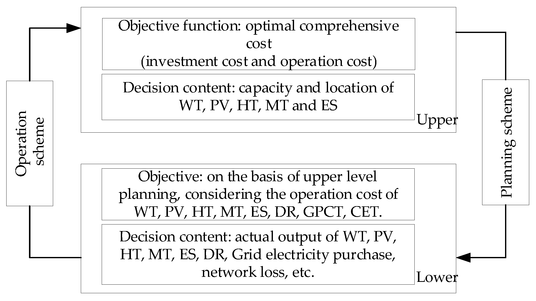
3. NDN Planning and Simulation Operation Bi-Layer Model

On the basis of the component model established in the previous section, a bi-layer model for the investment planning and simulation operation of an NDN was established. The bi-layer planning model used in this paper is shown in Equation (17): the upper layer is the investment decision layer, and the lower layer is the simulation operation layer. The upper layer transmits planning information to the lower layer, and the simulation operation results of the lower layer affect the upper-layer planning:
{ x Inv min F ( X Inv ) = C Inv G ( X Inv ) 0 H ( X Inv ) = 0 x Ope min F ( X Inv , X Ope ) = C Ope g ( X Inv , X Ope ) 0 h ( X Inv , X Ope ) = 0
In the formula: x Inv min F ( ) and x Ope min F ( ) are symbols of the objective function of investment and simulation operation; X Inv and X Ope are the investment variables and simulation operation variables; and C Inv and C Ope are the comprehensive investment cost and simulation operation cost of the NDN, respectively. G ( ) and H ( ) are investment constraints, while g ( ) and h ( ) are simulation operation constraints.

3.1. Acquisition Cost of Equipment in the Upper Layer

The equipment procurement cost considered in this paper is the procurement cost under the whole life cycle, including the initial investment cost, replacement cost and the residual value of the equipment at the end of the project cycle. C Inv is the annual fee, which calculates the annual cost of the equipment by averaging the total investment in equipment over its entire life cycle. The formula for annual equipment acquisition cost is:
C Inv = σ WT j G WT c WT n j , WT + σ PV j G PV c PV n j , PV + σ HT j G HT c HT n j , HT + σ MT j G MT c MT n j , MT + σ BAT j G BAT c BAT n j , BAT
σ = a ( 1 + a ) y ( 1 + a ) y 1
In the formula: G WT , G PV , G HT and G MT are a set of WT, PV, HT and MT investment candidate nodes; G BAT is the ES investment candidate node set; σ is the annual investment equivalence coefficient; σ WT , σ PV , σ HT and σ MT are the WT, PV, HT and MT annual investment equivalence coefficients; σ BAT is ES annual investment equivalence coefficient; a is the discount rate, the interest rate used to change the future payment to the present value; y is the service life of the equipment; c WT , c PV , c HT and c MT are the investment prices of the WT, PV, HT and MT units; n j , WT , n j , PV , n j , HT and n j , MT are the quantity of the WT, PV, HT and MT in the node j ; c BAT is the investment price of the ES unit; and n j , BAT is the quantity of ES in the node j .

3.2. Operating Costs at Lower Layer

Operation costs mainly include seven parts: (1) energy cost, including C grid buy : electricity purchase cost and C grid sale : electricity sales revenue; (2) C MT : MT operation cost; (3) C IBDR : compensation cost related to IBDR; (4) C LOSS : network loss cost; (5) C LoadGap : load fluctuation penalty cost; (6) C ED : CET cost; and (7) C G : GPCT revenue:
C Ope = C grid buy C grid sale + C IBDR + C LOSS + C MT + C LoadGap + C ED C G
C grid buy = t = 1 T c t buy P t buy Δ t
C grid sale = t = 1 T c t sale P t sale Δ t
C IBDR = t = 1 T λ IBDR L t D 0 Δ L t DR Δ t
C LOSS = c Loss t = 1 T i j E I ˜ i j , t r i j Δ t
C MT = t = 1 T j = 1 G MT ( c ( P j MT ( t ) ) Δ t + c S j MT ( t ) Δ t + k j P j MT ( t ) Δ t )
c S j MT ( t ) = max { 0 , β j ( t ) β j ( t 1 ) } C s , j MT
C LoadGap = c LoadGap t = 1 T ( j = 1 G Load P j , t , load DR + j = 1 G BAT P j , t , BAT , Cha j = 1 G BAT P j , t , BAT , Dis P Ave ) Δ t
In the formula: T is the collection of all the time periods; c t buy and c t sale are the purchase and sale price of electricity; P t buy and P t sale are the purchase and sale of electric power; and λ IBDR is the IBDR compensation unit price. E is the set of all branches in the NDN and c Loss is the unit price of the network loss penalty. The square of the branch i j current I 2 i j , t at the moment t , is represented by I ˜ i j , t ; the cost function can be linearized, and r i j is the branch resistance. G MT is the set of MT candidate investment nodes, G Load is the set of load nodes, and G BAT is the set of ES candidate investment node. c ( P j MT ( t ) ) is the fuel cost of the MT j in the time period t ; c S j MT ( t ) is the start-up cost of the MT j in the time period t ; C s , j MT is the cost of each start-up of the MT j ; k j is the maintenance cost of the MT j unit electric energy; P j MT ( t ) is the MT j generation; β j ( t ) is the start–stop state of the unit j in the time period t . A value of 0 means shutdown, while a value of 1 indicates that power is on; c LoadGap is the load fluctuation penalty; P j , t , load DR is the load demand of the node as j after participating in DR at time t , which is the joint action of PBDR and IBDR; P j , t , BAT , Cha and P j , t , BAT , Dis are the ES charge and discharge amount of the node j at time t ; and P Ave is the average load of the NDN.

4. Constraints of NDN Planning

4.1. Upper-Layer Investment Constraints

Due to the limitations of funds and sites, the WT, PV, HT, MT and ES that can be accessed by each node are limited. The investment constraints of WT, PV, HT, MT and ES are as follows:
{ 0 n j , WT N j , WT 0 n j , PV N j , PV 0 n j , HT N j , HT 0 n j , MT N j , MT 0 n j , BAT N j , BAT
In the formula: N j , WT , N j , PV , N j , HT , N j , MT are the upper limits of the number of WT, PV, HT and MT investments in the node j , and the investment capacity of WT, PV, HT and MT is an integer multiple of the capacity of a single machine; N j , BAT is the upper limit of the number of ES investments of the node j . ES investment capacity is also an integer multiple of the capacity of a single machine.

4.2. Lower-Layer Operating Constraints

The constraints are divided into eleven main categories: (1) second-order cone relaxation power flow constraints of NDN; (2) NDN security constraints; (3) power generation equipment capacity constraints; (4) power generation constraints; (5) MT constraints; (6) ES operation constraints; (7) power purchase and sales constraints with power grids; (8) NDN power balance constraints; (9) GPCT quotas and GPCT price constraints; (10) carbon emissions’ intensity constraints; and (11) GPCT and CET volume constraints.

4.2.1. Second-Order Cone Relaxation Power Flow Constraint of NDN

In this paper, the distflow branch power flow is used to constrain the power flow of the NDN, and the second-order cone relaxation (SOCR) technique is used to relax the original power flow model. For branches i j and j k , Λ ( j ) represents the set of starting points with node as the end point j , Ω ( j ) represents the set of end points with the node as the starting point j , and G E represents the set of all nodes of the NDN:
k = 1 Ω ( j ) P j k , t DR i = 1 Λ ( j ) ( P i j , t DR I ˜ i j , t r i j ) = j = 1 G BAT P j , t , BAT , Dis + j = 1 G WT P j , t , WT + j = 1 G PV P j , t , PV + j = 1 G HT P j , t , HT + j = 1 G MT P j , t , MT
U ˜ j , t = U ˜ i , t 2 ( P i j , t DR r i j Q i j , t x i j ) + I ˜ i j , t ( r i j 2 + x i j 2 )
2 P i j , t DR 2 Q i j , t I ˜ i j , t U ˜ j , t 2 I ˜ i j , t + U ˜ j , t
In the formula: i , j G E , P i j , t DR and Q i j , t are the active power and reactive power of the branch i j after participating in the DR at the moment t , assuming that participating in the DR does not affect the reactive power; P j k , t DR is the active power of the branch j k participating in the DR at the moment; P j , t , WT , P j , t , PV , Pj,i,HT are the generated power of WT, PV, HT of the node j at the moment t ; G WT , G PV , G HT are the investment candidate node set of WT, PV, HT; x i j is the reactance of the branch i j ; U ˜ i , t and U ˜ j , t are the voltage square of the node i j at the moment t .

4.2.2. NDN Security Constraints

{ U j , min U j , t U j , max I i j , t I i j , max
In the formula: U j , max , U j , min are the upper and lower limits of the voltage amplitude of the network node j , respectively; I i j , max is the upper limit of the branch i j current amplitude.

4.2.3. Power Generation Equipment Apparent Power Capacity Constraints

S G , n cap , min S G , n cap S G , n cap , max
In the formula, S G , n cap , min and S G , n cap , max are the minimum and maximum apparent power capacity of the WT, PV, HT, and MT equipment n , and S G , n cap is the apparent power capacity of the equipment n .

4.2.4. Power Generation Constraints

In the NDN, considering the characteristics of power generation equipment and the safety and reliability of the NDN, the power of the equipment must be limited between the minimum output power and the rated power:
δ n S G , n cap v n min cos ϕ n P t E n δ n S G , n cap cos ϕ n
Assuming ξ n = δ n S G , n cap cos ϕ n , Equation (34) can be expressed as:
{ ξ n v n min P t E n ξ n δ n v G , n cap , min ξ n δ n v G , n cap , max ( 1 δ n ) S G , n cap , min cos ϕ n S G , n cap cos ϕ n ξ n ( 1 δ n ) S G , n cap , max cos ϕ n
In the formula: δ n is the binary variables that determine the operating state of the equipment n , v n min is the minimum output power coefficient of the equipment n , cos ϕ n is the power factor of the equipment n , P t E n is the output of the equipment n , and ξ n is the linearization auxiliary variables.

4.2.5. MT Constraints

The main constraints are power output constraints, climbing constraints, and start–stop time constraints:
P j , min MT β j ( t ) P j MT ( t ) P j , max MT β j ( t )
R j down Δ T P j MT ( t ) P j MT ( t 1 ) R j up Δ T
( T j on ( t 1 ) T j U ) ( β j ( t 1 ) β j ( t ) ) 0
( T j off ( t 1 ) T j D ) ( β j ( t ) β j ( t 1 ) ) 0
In the formula, P j , min MT , P j , max MT are the minimum and maximum outputs of the MT j ; R j down , R j up are the downward and upward climbing speeds of the MT j ; T j on , T j off are the continuous on–off state time of unit j in the period of time t ; T j U , T j D are the minimum continuous on–off time of unit j .

4.2.6. ES Operation Constraints

The constraints on ES can be expressed as follows:
{ 0 P t , Cha δ Cha P max BAT 0 P t , Dis δ Dis P max BAT δ Cha + δ Dis = { 0 , 1 } E min E t E max
In the formula, P t , Cha and P t , Dis are the ES charge and discharge power, δ Cha and δ Dis are the binary variables of the ES charge and discharge, P max BAT is the maximum charge and discharge power, and E min and E max are the ES minimum and maximum capacity.

4.2.7. Power Purchase and Sales Constraints with Power Grids

The energy exchange between the NDN and the large grid has capacity constraints:
G max p t buy G max

4.2.8. NDN Power Balance Constraints

The NDN should satisfy the power balance, which can be expressed by the following equation:
δ b u y P t buy + P t , PV + P t , WT + P t , HT + P t , MT + P t , Dis = P t , Cha + δ sale P t sale + L t D 0
δ b u y + δ sale = { 0 , 1 }

4.2.9. GPCT Quotas and GPCT Price Constraints

E m A k g = n S re k n g E m n + G m buy G m sale
A 30 %
In the formula, A is the quota coefficient of NE, that is, the part of the electricity supplied through the NE in a certain year. The NDN in this paper requires the quota coefficient to be higher than 30%. E m is the supply of electricity in the m year, MWh; E m n is the power generation of NE generators n in the m year; S re indicates generators belonging to NE; k n g is the green power certificate number that renewable energy can obtain; G m buy and G m sale are the green power certificates bought and sold in the m year:
c m , min G = ( s l s c ) ( 1 + r l ) ( h l + d l )
c m , max G = ( s l s c )
In the formula: c m , min G is the lower limit of GPCT price; c m , max G is the upper limit of GPCT price; s l is the electricity price of the NE l ; sc is the benchmark electricity price for local thermal power; r l is the discount rate of the NE l ; hl is the payment cycle of fiscal subsidy for the NE l ; d l is delay the payment period for the fiscal subsidy of the NE l .

4.2.10. Carbon Emissions Intensity Constraints

To achieve the “dual carbon” goal and reduce the carbon emissions of the NDN, the Government will set a carbon emissions limit for the NDN. When the actual emissions amount exceeds the emissions limit, the NDN company needs to purchase the excess from the market; when the actual emissions amount is lower than the emissions limit, the NDN company can sell the remaining part of the quota in the market:
μ m C O 2 Q m E = E q , m + C m buy C m sale
μ m C O 2 0.1   t / MWh
In the formula: Q m E is the total electricity consumption of the NDN in the year m , μ m C O 2 is the carbon emissions intensity of the average unit power supply of the NDN in the year m , E q , m is the total carbon emissions quota limit of the NDN in the year m , t; C m buy and C m sale represent the year m of the NDN carbon emissions from buying and selling, t.

4.2.11. GPCT and CET Volume Constraints

{ G m buy 0 G m sale 0 C m buy 0 C m sale 0
In the formula, G m buy and G m sale represent the numbers of green power certificates bought and sold in year m , respectively. C m buy and C m sale represent the carbon emissions purchased and sold by the NDN in year m , respectively.

5. Bi-Layer Programming Model Transformation

The upper layer plans the capacity and location of WT, PV, HT, MT, and ES. Decision content: capacity and location of WT, PV, HT, MT and ES installations. The lower-layer operation considers the operating costs of WT, PV, HT, MT, ES and load DR. Decision content: the actual output of WT, PV, HT, MT, ES, DR power, electricity purchased and sold with the main grid, network loss, load fluctuation, etc. According to Formula (17), it can be seen that the proposed objective function is a bi-layer, with the investment decision of the upper layer and the simulation operation of the lower layer. The planning capacity and location of the upper layer are transferred to the lower layer, and the operation cost of the lower layer is transferred to the upper layer. The planning result can be obtained when the system is optimized. The specific goals and contents of each layer are shown in Figure 1.
The upper layer is a long-time-scale programming model; the lower layer is a short-time-scale simulation operation optimization scheme. The upper layer of the bi-layer model includes integer variables and continuous variables, and the lower layer is a mixed-integer nonlinear programming (MINLP) problem. There is a coupling relationship between the upper and lower models, which is difficult to directly solve. Since the lower layer belongs to convex optimization, the KKT condition is a sufficient and necessary condition for the optimality of the solution of the convex optimization problem. In this paper, the single-layer transformation method is used to construct the Lagrangian function of the lower-layer model. Based on the KKT condition of the lower-layer model, the lower-layer model is converted to the constraints of the upper model, while the bi-layer model is transformed into a single-layer, nonlinear programming model. Then, the Big-M method is used to linearize the nonlinear part of the transformed, single-layer, nonlinear model to form a single-layer MISOCP problem [31]. For details on the transformation process, please refer to the Appendix A. In Matlab2016b, the YALMIP toolbox and the CPLEX12.7 solver are used to solve the problem. The specific process is shown in Figure 2.

6. Cases

6.1. Introduction to Case Environment and Parameters

In this paper, the planning calculation is based on the modified IEEE33 node system. Parameters such as the planned operation period, discount rate, load data, line-loss cost, and upper and lower limits of voltage and current are derived from the literature [6]. Using the abundant wind–solar–water resources data in Southwest China, and comprehensively considering energy distribution and energy demand in the planning area, WT, PV, HT, MT and ES investment candidate nodes are derived from the literature [7], as shown in Figure 3. ES charge and discharge are calculated by time-of-use electricity price, and the relevant data for GPCT and CET are derived from the literature [28]. The price elasticity is also derived from the literature [12]. The total planning period is 10 years, and the optimization scheduling period is also 10 years, with 4 typical days of spring, summer, autumn and winter considered in the annual operation optimization. The article displays the simulation operation results on a typical day in summer.

6.2. Analysis of Planning Results

6.2.1. Planning Results of NDN Considering GPCT and CET

The results of the NDN planning considering GPCT and CET are shown in Table 1 and Table 2. Since the investment cost of WT and HT is lower than that of PV, the investment of WT and HT reaches the planned upper limits of 2.5 MW × 3 and 10 MW. Due to the high operating costs of MT, the installed capacity is planned to be only 7 MW. The PV of nodes 24 and 31 is closer to ES, and the fluctuation in PV output can be reduced through ES, so the planned capacity is 2.5 MW. The distance between 10-node PV and 6-node HT is relatively small, and the output of the HT is larger, so the planned capacity of 10-node PV is 1.1 MW. The proportion of the installed capacity of renewable energy in the planned NDN reaches 77.12% and is close to the 80% requirement of a “carbon neutral” renewable-energy installation capacity, which experts expect to be achieved by 2060 [32].

6.2.2. NDN Simulation Operation Considering GPCT and CET

The simulation results are shown in Figure 4 and Figure 5. The peak–valley difference between the original load is 14.1195 MW, and the peak–valley difference between the after PBDR load is 12.0884 MW, with a reduction of 14.39%. After adjusting for ES and IBDR, the peak–valley difference becomes 9.3911 MW, which is 33.49% lower than the original load. ES charges at 1:00–10:00 when the TOU price is low (low load), and discharges at 11:00–23:00 when TOU price is high (high load), which can reduce the load peak–valley difference. The same can be said of IBDR, which has no investment cost, but an operating cost.
The HT output is relatively stable, and the power generation cost is low, so the HT is planned according to the long-term maximum, full running capacity. The wind is strong at night and low in the daytime. PV generation is from 6:00 to 19:00 in the daytime. WT and PV are somewhat complementary. During the load peak period from 15:00 to 22:00 in the evening, the power supply is supplemented by the MT. The running time of the MT is from 10:00 to 24:00. Due to the MT climbing constraints, the power peak is insufficient from 17:00 to 20:00 and from 20:00 to 22:00. The NDN will purchase power from the superior grid to meet the balance between supply and demand. At other times, when the power generation of the NDN exceeds the load, it will sell power to the superior grid to obtain additional income.
The output of non-water renewable energy, water-bearing renewable energy and MT accounts for 48.94%, 90.39% and 9.61% of the NDN. The overall carbon emissions of the NDN are 24.04 g/kWh, close to zero-carbon emissions.

6.2.3. Comparative Analysis of GPCT, CET and the Traditional Model Are Considered

TDN planning, without considering DR, GPCT and CET, is taken as a reference, and factors such as DR, GPCT and CET are considered as comparative calculation examples, as shown in Table 3.
According to the investment and simulation results in Table 3, the traditional planning income of scheme 1, excluding DR, GPCT and CET, is CNY 136.38 million, but it cannot meet the requirements of the NE consumption quota of the NDN, or the carbon emissions intensity of average unit power supply required by the NDN. Compared with the planning of GPCT and CET, scheme 3, which includes DR and excludes the planning of GPCT and CET, improves the overall income by 38.10%. Compared with scheme 1, scheme 2, excluding DR and considering the planning of GPCT and CET, improves the overall income by 69.99%. Compared with scheme 4, the planning of DR, GPCT and CET with scheme 1, the total planning cost is the lowest and the total revenue is the highest, at CNY 282.82 million. The specific results are shown in Table 1 and Table 2. The overall revenue increases by 107.38%, the output proportion of water-bearing renewable energy is 90.39%, and the average carbon emissions intensity is 24.04 g/kWh. This can meet both the NE consumption quota of the NDN and the carbon emissions intensity requirement of the average unit power supply of the NDN. The NDN profits by selling the excess green power certificate quota and carbon quota.

6.2.4. Price Sensitivity Analysis of GPCT and CET

As can be seen from Table 3, in the NDN, an important part of the income is the income from GPCT and CET; GPCT accounts for a higher proportion of income than CET. Scheme 5 considers the revenue of GPCT to be CNY 279.83 million, and scheme 6 considers the revenue of CET to be CNY 192.87 million. The former has a greater impact on NDN planning than the latter, because the NDN that is mainly based on NE has a lower carbon emissions quota and lower CET volume.
The impact of price changes in GPCT and CET on planning is shown in Figure 6. As can be seen from Figure 6, the investment cost of WT and HT is low, and the maximum capacity is planned in various planning processes. The PV cost is high, and the GPCT price of PV is also high. The GPCT price of PV will greatly affect the planned capacity of PV, and the planned capacity of PV is positively correlated with the GPCT price of PV. When the price of GPCT and CET ranges from 0 to 0.9 times, the planned PV capacity increases and the total revenue increases accordingly. When the price of GPCT and CET increases from 0.9 times to once, MT capacity planning begins to decrease. The reason for this is that the increase in the price of GPCT increases PV installation, and the total revenue increases faster than the revenue provided by MT. GPCT has a more sensitive impact on NDN planning than CET. When the price of GPCT and CET increases from 1.1 to 1.2 times, with the increase in GPCT income, the planning PV capacity further increases, and the total income increases, further reducing MT and HT planning. When the price of GPCT and CET increases from 1.2 to 1.3 times, PV capacity reaches the planning limit and cannot continue to increase.

6.2.5. Algorithm Performance Analysis

The model in this paper is essentially a MINLP model before the linearization and second-order cone relaxation process [6], which can usually be solved by a genetic algorithm and the Bonmin toolkit. After linearization and second-order cone relaxation, the model is transformed into a MISOCP model that can be solved by CPLEX, which is the solution route adopted in this paper. To verify the validity of the model and algorithm in this paper, we simultaneously adopted the above two solution routes and compared the solution time of the three methods, as shown in Table 4. An analysis of Table 4 shows that the Bonmin toolkit cannot solve the model, and the solving process of the genetic algorithm takes a long time, while the CPLEX optimization package can solve the problem relatively quicker.

6.3. PG&E69 NDN System

To verify the applicability of the proposed planning model to larger-scale system, we describe the planning of the PG&E69 NDN system with the proposed model and algorithm in this section. The main parameters of the PG&E69 NDN system are from reference [33], and the rest parameters are the same as the IEEE33 node system. The planning and simulation results are shown in Table 5 and Table 6.
The proportion of the installed capacity of renewable energy in the planned NDN reaches 73.79%, which is close to the proportion needed to reach “carbon neutral” by 2060, that is 80% [32]. The output of non-water renewable energy, water-bearing renewable energy and MT accounts for 43.45%, 84.28% and 15.72% of the NDN, respectively. The overall carbon emission of the NDN is 30.16 g/kWh, close to zero-carbon emissions. Through the above analyses, the proposed planning and simulation operation model is also applicable to the PG&E69 NDN system.

7. Conclusions

(1)
On the basis of the GPCT and CET model, the average carbon emissions intensity of the power supply unit of the NDN is introduced to organically combine the influences of GPCT and CET on the NDN planning, and the role of DR is also included. Compared with considering the influences of the three models alone, the planning results are as follows: The proportion of NE installed in the NDN, carbon emissions intensity per power supply unit and total income of the NDN were greatly improved. More specifically, the proportion of installed NE and the carbon emissions intensity per power supply unit essentially reached the NDN goal of “carbon neutrality”, and they could profit by selling the excess green power certificate quota and carbon quota at the same time.
(2)
It can be seen that the participation of NDN in GPCT accounts for a higher proportion than CET, and GPCT has a greater impact on NDN planning than CET, mainly because the GPCT price of PV is higher and has a greater impact on the distributed PV-planning capacity of NDN, while CET has a greater impact on the distributed MT planning capacity of NDN. It can be seen from the calculation results that the sensitivity of GPCT price to NDN planning is greater than that of CET. Next, we can further study the proportion of NDN to preferentially participate in GPCT and CET, to increase income and lower carbon emissions.
(3)
The planning model is suitable for regions with abundant wind, solar, and water resources. For regions without one or more of these three renewable resources, the planning economic benefits of the model will decrease, and the intensity of carbon emissions will increase. The results of this example verify the rationality and applicability of the model, and the research results can provide a reference for NDN planning in areas with abundant wind, solar, and water resources.
(4)
This paper mainly considers NDN planning; the uncertainties of the distributed generation and loads are not reflected in this paper. We look forward to considering the uncertainties of the distributed generation and loads in further research.

Author Contributions

Conceptualization, H.W., X.S. and J.L.; methodology, H.W. and X.S.; software, H.W.; validation, H.W., X.S. and J.L.; formal analysis, H.W. and X.S.; investigation, H.W. and X.S.; resources, J.L.; data curation, H.W.; writing—original draft preparation, H.W.; writing—review and editing, H.W., X.S. and J.L.; visualization, H.W.; supervision, X.S.; project administration, X.S.; funding acquisition, J.L. All authors have read and agreed to the published version of the manuscript.

Funding

This research was funded by the National Natural Science Foundation of China, grant number U2066209 from January 2021 to December 2024, and this research was funded by the China Southern Power Grid Major Science and Technology Special Project, grant number 060400KK52190017.

Institutional Review Board Statement

Not applicable.

Informed Consent Statement

Not applicable.

Conflicts of Interest

The authors declare no conflict of interest.

Appendix A

First, Lagrangian multipliers are introduced in the lower-layer model, and the equality and inequality constraints are transformed into standard forms, respectively; the Lagrangian function (A1) is correspondingly obtained. Then, according to the obtained Lagrangian function (A1) and the lower-layer KKT complementary relaxation conditions, the lower-layer model can be transformed into the upper-layer model’s constraints (A4)–(A29), where (A2) and (A3) are the objective function and constraint of the original upper-layer model, respectively.
C Ope = t = 1 T ( c t buy P t buy c t sale P t sale + j = 1 G MT ( c ( P j MT ( t ) ) + max { 0 , β j ( t ) β j ( t 1 ) } C s , j MT + k j P j MT ( t ) ) + c Load i j E I ˜ i j , t r i j + c LoadGap ( j = 1 G Load P j , t , load DR + j = 1 G BAT P j , t , BAT , Cha j = 1 G BAT P j , t , BAT , Dis P Ave ) + c t ED ( μ E μ D ) P t buy + c t G k g ( G gre , t - A Q t ) + λ IBDR L t D 0 Δ L t DR ) Δ t + λ 1 , i , j , t ( k = 1 Ω ( j ) P j k , t DR i = 1 Λ ( j ) ( P i j , t DR I ˜ i j , t r i j ) j = 1 G BAT P j , t , BAT , Dis j = 1 G WT P j , t , WT j = 1 G PV P j , t , PV j = 1 G HT P j , t , HT j = 1 G MT P j , t , MT ) + λ 2 , i , j , t ( U ˜ j , t U ˜ i , t + 2 ( P i j , t DR r i j Q i j , t x i j ) I ˜ i j , t ( r i j 2 + x i j 2 ) ) μ 1 , , i , j , t min ( I ˜ i j , t + U ˜ j , t 2 P i j , t DR 2 Q i j , t I ˜ i j , t U ˜ j , t 2 ) + μ 2 , i , j , t min ( U j , min U j , t ) + μ 2 , i , j , t max ( U j , t U j , max ) + μ 3 , i , j , t max ( I i j , t I i j , max ) + μ 4 , i , j , t min ( S G , n cap , min S G , n cap ) + μ 4 , i , j , t max ( S G , n cap S G , n cap , max ) + μ 5 , i , j , t min ( δ n S G , n cap v n min cos ϕ n P t E n ) + μ 5 , i , j , t max ( P t E n δ n S G , n cap cos ϕ n ) + μ 6 , i , j , t min ( P j , min MT β j ( t ) P j MT ( t ) ) + μ 6 , i , j , t max ( P j MT ( t ) P j , max MT β j ( t ) ) + μ 7 , i , j , t min ( R j down Δ T P j MT ( t ) + P j MT ( t 1 ) ) + μ 7 , i , j , t max ( P j MT ( t ) P j MT ( t 1 ) R j up Δ T ) μ 8 , i , j , t min ( ( T j on ( t 1 ) T j U ) ( β j ( t 1 ) β j ( t ) ) ) μ 9 , i , j , t min ( ( T j off ( t 1 ) T j D ) ( β j ( t ) β j ( t 1 ) ) ) + μ 10 , i , j , t min ( 0 P t , Cha ) + μ 10 , i , j , t max ( P t , Cha δ Cha P max BAT ) + μ 11 , i , j , t min ( 0 P t , Dis ) + μ 11 , i , j , t max ( P t , Dis δ Dis P max BAT ) + μ 12 , i , j , t min ( E min E t ) + μ 12 , i , j , t max ( E t E max ) + λ 3 , i , j , t ( ( δ Cha + δ Dis ) { 0 , 1 } ) + μ 13 , i , j , t min ( G max p t buy ) + μ 13 , i , j , t max ( p t buy G max ) + λ 4 , i , j , t ( δ b u y P t buy + P t , PV + P t , WT + P t , HT + P t , MT + P t , Dis P t , Cha δ sale P t sale L t D 0 ) + λ 5 , i , j , t ( δ b u y + δ sale { 0 , 1 } ) + λ 6 , i , j , t ( E m η m k g n S re k n g E m n G m buy + G m sale ) + λ 8 , i , j , t ( c max G ( s l s c ) ) + λ 7 , i , j , t ( c min G ( s l s c ) / ( 1 + r l ) ( h l + d l ) ) + λ 9 , i , j , t ( μ m CO 2 Q m E E q , m C m buy + C m sale ) + + μ 14 , i , j , t min ( 30 % A ) + μ 15 , i , j , t max ( μ m CO 2 0.1 ) μ 16 , i , j , t min G m buy μ 17 , i , j , t min G m sale μ 18 , i , j , t min C m buy μ 19 , i , j , t min C m sale
{ C Inv = σ WT j G WT c WT n j , WT + σ PV j G PV c PV n j , PV + σ HT j G HT c HT n j , HT + σ MT j G MT c MT n j , MT + σ BAT j G BAT c BAT n j , BAT σ = a ( 1 + a ) y ( 1 + a ) y 1
{ 0 n j , WT N j , WT 0 n j , PV N j , PV 0 n j , HT N j , HT 0 n j , MT N j , MT 0 n j , BAT N j , BAT
0 μ 1 , i , j , t min ( I ˜ i j , t + U ˜ j , t 2 P i j , t DR 2 Q i j , t I ˜ i j , t U ˜ j , t 2 ) 0
0 μ 2 , i , j , t min ( U j , t U j , min ) 0
0 μ 2 , i , j , t max ( U j , max U j , t ) 0
0 μ 3 , i , j , t max ( I i j , max I i j , t ) 0
0 μ 4 , i , j , t min ( S G , n cap S G , n cap , min ) 0
0 μ 4 , i , j , t max ( S G , n cap , max S G , n cap ) 0
0 μ 5 , i , j , t min ( P t E n δ n S G , n cap v n min cos ϕ n ) 0
0 μ 5 , i , j , t max ( δ n S G , n cap cos ϕ n P t E n ) 0
0 μ 6 , i , j , t min ( P j MT ( t ) P j , min MT β j ( t ) ) 0
0 μ 6 , i , j , t max ( P j , max MT β j ( t ) P j MT ( t ) ) 0
0 μ 7 , i , j , t max ( R j up Δ T P j MT ( t ) + P j MT ( t 1 ) ) 0
0 μ 8 , i , j , t min ( ( T j on ( t 1 ) T j U ) ( β j ( t 1 ) β j ( t ) ) ) 0
0 μ 9 , i , j , t min ( ( T j off ( t 1 ) T j D ) ( β j ( t ) β j ( t 1 ) ) ) 0
0 μ 10 , i , j , t min ( P t , Cha 0 ) 0
0 μ 10 , i , j , t max ( δ Cha P max BAT P t , Cha ) 0
0 μ 11 , i , j , t min ( P t , Dis 0 ) 0
0 μ 11 , i , j , t max ( δ Dis P max BAT P t , Dis ) 0
0 μ 12 , i , j , t min ( E t E min ) 0
0 μ 13 , i , j , t min ( p t buy + G max ) 0
0 μ 13 , i , j , t max ( G max p t buy ) 0
0 μ 14 , i , j , t min ( A 30 % ) 0
0 μ 15 , i , j , t max ( 0.1 μ m CO 2 ) 0
0 μ 16 , i , j , t min G m buy 0
0 μ 17 , i , j , t min G m sale 0
0 μ 18 , i , j , t min C m buy 0
0 μ 19 , i , j , t min C m sale 0
The meaning of the formula “0 ≤ a ⊥ b ≥ 0” is that a ≥ 0, b ≥ 0 and a × b = 0.
In the converted single-layer model (A2)–(A29), the constraints (A4)–(A29) are nonlinear constraints. By using the Big-M method and introducing several 0–1 variables, the original nonlinear constraints are equivalently transformed into mixed-integer second-order cone constraints, and constraint (A5) is transformed into constraints (A30) and (A31) as an example to introduce, the transformation of the other constraints among (A4)–(A29) is similar to the transformation of constraint (A5).
0 μ 2 , i , j , t min M u min v u , i , j , t min
0 U j , t U j , min M u min ( 1 v u , i , j , t min )
In the formula: M u min is a sufficiently large constant and v u , i , j , t min is a binary variable.

References

  1. Zeng, M.; Wang, Y.L.; Zhang, S.; Liu, Y.X. “14th Five-Year” energy plan and “30·60” dual-carbon goals in the process of achieving 12 key issues. China Power Enterp. Manag. 2021, 1, 41–43. [Google Scholar]
  2. Perdan, S.; Azapagic, A. Carbon trading: Current schemes and future developments. Energy Policy 2011, 39, 6040–6054. [Google Scholar] [CrossRef]
  3. Zhou, J.; Deng, Y.R.; Zhuang, C.W. Development Process, Current Situation and Prospect of China’s Carbon Trading Market. Environ. Sci. Manag. 2020, 45, 1–4. [Google Scholar]
  4. Quan, S. Active Power Distribution System Planning Considering Demand-Side Resource Integration; China Electric Power Research Institute: Beijing, China, 2019. [Google Scholar]
  5. Qi, N.; Cheng, L.; Tian, L.T.; Guo, J.B.; Huang, R.L.; Wang, C.P. Review and Prospect of Distribution Network Planning Research Considering Access of Flexible Load. Autom. Electr. Power Syst. 2020, 44, 193–207. [Google Scholar]
  6. Gao, H.J.; Liu, J.Y. Coordinated Planning Considering Different Types of DG and Load in Active Distribution Network. Proc. CSEE 2016, 36, 4911–4922. [Google Scholar]
  7. Liu, J.Y.; Lu, L.; Gao, H.J.; Liu, J.Y.; Shi, W.C.; Wu, Y. Planning of Active Distribution Network Considering Characteristics of Distributed Generator and Electric Vehicle. Autom. Electr. Power Syst. 2020, 44, 41–48. [Google Scholar]
  8. Zhang, Y.H.; Lu, L.; Pan, C.; Zhang, Y.P.; Luo, Y.X.; Bao, F. Planning strategies of source-storage considering wind-photovoltaic-load time characteristics. Power Syst. Prot. Control 2020, 48, 48–56. [Google Scholar]
  9. Zeng, B.; Zhang, J.; Yang, X.; Wang, J.; Dong, J.; Zhang, Y. Integrated Planning for Transition to Low-Carbon Distribution System with Renewable Energy Generation and Demand Response. IEEE Trans. Power Syst. 2014, 29, 1153–1165. [Google Scholar] [CrossRef]
  10. Cheng, L.; Qin, N.; Tian, L.T. Joint Planning of Generalized Energy Storage Resource and Distributed Generator Considering Operation Control Strategy. Autom. Electr. Power Syst. 2019, 43, 27–35. [Google Scholar]
  11. Liu, H.; Zheng, N.; Ge, S.Y.; Xu, Z.Y.; Guo, L. Coordinated Planning of Source and Network in Active Distribution System with Demand Response and Optimized Operation Strategy. Autom. Electr. Power Syst. 2020, 44, 89–97. [Google Scholar]
  12. Xiang, Y.; Cai, H.; Gu, C.; Shen, X. Cost-benefit analysis of integrated energy system planning considering demand response. Energy 2020, 192, 116632. [Google Scholar] [CrossRef]
  13. Huang, Z.L.; Jiang, X.B.; Liu, L.J. Multi-objective optimal allocation of “generation-storage-load” under the low-carbon background. J. Electr. Power Sci. Technol. 2020, 35, 36–45. [Google Scholar]
  14. Zhang, X.H.; Yan, P.D.; Zhong, J.Q.; Lu, Z.G. Research on Generation Expansion Planning in Low-Carbon Economy Environment Under Incentive Mechanism of Renewable Energy Sources. Power Syst. Technol. 2015, 39, 655–662. [Google Scholar]
  15. Zhang, G.; Zhang, F.; Zhang, L.; Liang, J.; Han, X.; Yang, Y. Two-stage Robust Optimization Model of Day-ahead Scheduling Considering Carbon Emissions Trading. Proc. CSEE 2018, 38, 5490–5499. [Google Scholar]
  16. Cao, J.W.; Mu, C.W.; Sun, K.; Tan, J.J.; Zhang, Q.M.; Cui, X.; Bai, Y. Optimal configuration method of wind-photovoltaic-storage capacities for regional power grid considering carbon trading. Eng. J. Wuhan Univ. 2020, 53, 1091–1096+1105. [Google Scholar]
  17. Zhu, W.Y.; Luo, Y.; Hu, B.; Luo, H.H.; Zhang, Y.; Han, Y.; Tang, M.Y.; Tong, Q.D. Optimized Combined Heat and Power Dispatch Considering Decreasing Carbon Emission by Coordination of Heat Load Elasticity and Time-of-Use Demand Response. Power Syst. Technol. 2021, 45, 3803–3813. [Google Scholar]
  18. Huang, C. The Effect of Carbon Emission Policies on Decision-making of Clean Power Generation Technologies Investment. Yuejiang Acad. J. 2019, 11, 39–51+122. [Google Scholar]
  19. Zhou, X.; James, G.; Liebman, A.; Dong, Z.Y.; Ziser, C. Partial Carbon Permits Allocation of Potential Emission Trading Scheme in Australian Electricity Market. IEEE Trans. Power Syst. 2010, 25, 543–553. [Google Scholar] [CrossRef]
  20. Luo, Z.; Qin, J.; Liang, J.; Zhao, M.; Wang, H.; Liu, K. Operation Optimization of Integrated Energy System with Green Certificate Cross-chain Transaction. Power Syst. Technol. 2021, 2, 1–11. [Google Scholar]
  21. Yao, J.; He, J.; Wu, Y.F.; Yan, C.X. Energy Optimization of Electricity Wholesale Market with Carbon Emissions Trading and Green Power Certificate Trading System. Electr. Power 2021, 1–9. [Google Scholar]
  22. Wei, Z.; Wei, P.; Guo, Y.; Huang, Y.; Lu, B. Decentralized Low-carbon Economic Dispatch of Electricity-gas Network in Consideration of Demand-side Management and Carbon Trading. High Volt. Eng. 2021, 47, 33–47. [Google Scholar]
  23. Yu, X.; Dong, Z.; Zhou, D.; Sang, X.; Chang, C.T.; Huang, X. Integration of tradable green certificates trading and carbon emissions trading: How will Chinese power industry do? J. Clean. Prod. 2021, 279, 123485. [Google Scholar] [CrossRef]
  24. Bartolini, A.; Mazzoni, S.; Comodi, G.; Romagnoli, A. Impact of carbon pricing on distributed energy systems planning. Appl. Energy 2021, 301, 117324. [Google Scholar] [CrossRef]
  25. Liu, Q.H.; Yuan, H.; Yang, Z.L.; Fan, H.F.; Xu, C.L. Discussion on Compensation Ancillary Service Scheme of Green Certificates Based on Renewable Portfolio Standard. Autom. Electr. Power Syst. 2020, 44, 1–8. [Google Scholar]
  26. National Development and Reform Commission. National Energy Administration. Notice on Establishing and Improving Renewable Energy Power Consumption Guarantee Mechanism. Available online: http://www.china-nengyuan.com/exhibition/china-nengyuan_exhibition_news_139370.pdf (accessed on 10 March 2022).
  27. Zhang, X.H.; Yan, K.K.; Lu, Z.G.; He, S.L. Low-carbon economic dispatch of wind power system based on carbon trading. Power Syst. Technol. 2013, 37, 2697–2704. [Google Scholar]
  28. Ministry of Ecology and Environment of the People’s Republic of China. Baseline Emission Factors of China’s Regional Power Grid for the 2019 Emission Reduction Project. Available online: http://www.Mee.gov.cn/ywgz/ydqhbh/wsqtkz/202012/t20201229_815386.shtml (accessed on 10 March 2022).
  29. Wang, W.L.; Zhou, M.X.; Guan, Q.; Luo, Y.X.; Xu, X.L. Research and practice of optimum operation method based on genetic algorithm for small hydropower stations. J. Hydroelectr. Eng. 2005, 24, 6–11. [Google Scholar]
  30. Wu, X.; Wang, X.; Wang, J.; Bie, Z. Economic Generation Scheduling of a Microgrid using Mixed integer programming. Proc. CSEE 2013, 33, 1–9. [Google Scholar]
  31. Wu, S.J.; Li, Q.; Liu, J.K.; Zhou, Q.; Wang, C.G. Bi-level Optimal Configuration for Combined Cooling Heating and Power Multi-microgrids Based on Energy Storage Station Service. Power Syst. Technol. 2021, 45, 3822–3832. [Google Scholar] [CrossRef]
  32. Zhuo, Z.Y.; Zhang, N.; Xie, X.R.; Li, H.Z.; Kang, C.Q. Key Technologies and Developing Challenges of Power System with High Proportion of Renewable Energy. Autom. Electr. Power Syst. 2021, 45, 171–191. [Google Scholar]
  33. Alam, M.S.; Arefifar, S.A. Hybrid PSO-TS Based Distribution System Expansion Planning for System Performance Improvement Considering Energy Management. IEEE Access 2020, 8, 221599–221611. [Google Scholar] [CrossRef]
Figure 1. The objective function and decision content of the planning model.
Energies 15 02435 g001
Figure 2. Model processing and solving.
Energies 15 02435 g002
Figure 3. Candidate locations for WT, PV, HT, MT and ES stations.
Energies 15 02435 g003
Figure 4. Typical daily simulation results.
Energies 15 02435 g004
Figure 5. ES and IBDR simulation operation.
Energies 15 02435 g005
Figure 6. The impact of GPCT and CET price changes on planning.
Energies 15 02435 g006
Table 1. IEEE33 NDN planning results considering GPCT and CET.
EquipmentQuantity (Location)Capacity/MW
ES6 (5)1.08
ES5 (16)0.9
ES6 (25)1.08
ES5 (33)0.9
WT25 (3)2.5
WT25 (17)2.5
WT25 (21)2.5
PV11 (10)1.1
PV25 (24)2.5
PV25 (31)2.5
HT10 (6)10
MT7 (2)7
Table 2. IEEE33 NDN planning and simulation operation cost considering GPCT and CET.
Cost ItemInvestment (CNY 10,000)Operation (CNY 10,000)
ES1344
WT11,250
PV15,250
HT15,000
MT2100
IBDR 0.1261
Natural gas 2.2129
Load fluctuation 5.0027
Network loss 1.1318
GPCT (wind) −1.6289
GPCT (solar) −2.3635
CET −0.0852
Grid electricity purchase −4.8850
Running cost 1 d −0.4891
Investment cost 10 y44,944
Running cost 10 y −1785.22
Total cost 10 y43,158.79
Electricity sales revenue 10 y71,440.36
Total revenue 10 y28,281.57
Table 3. Planning case comparison.
SchemeDRGPCTCETIncome
(CNY 10,000)
1nonono13,638
2noyesyes23,183
3yesnono18,834
4yesyesyes28,282
5yesyesno27,983
6yesnoyes19,287
Table 4. Comparison of solving efficiency of different algorithms.
Model CategorySolution AlgorithmSolution Time
MINLPBonminInfeasible
MINLPGenetic Algorithm>2 h
MISOCPCPLEX128.56 s
Table 5. PG&E69 NDN planning results considering GPCT and CET.
EquipmentQuantity
(Location)
Capacity/MWEquipmentQuantity
(Location)
Capacity/MW
ES5(2)0.9WT25 (49)2.5
ES4(9)0.72WT25 (61)2.5
ES6(12)1.08PV18 (7)1.8
ES5(23)0.9PV20 (20)2.0
ES6(31)1.08PV25 (31)2.5
ES6(49)1.08PV25 (49)2.5
ES4(65)0.72PV16 (65)1.6
WT21(3)2.1HT15 (9)15
WT21(11)2.1MT6 (2)6
WT20(21)2.0MT7 (47)7
Table 6. PG&E69 NDN planning and simulation operation cost considering GPCT and CET.
Cost ItemInvestment (CNY 10,000)Operation (CNY 10,000)
ES2199
WT16,800
PV26,000
HT22,500
MT3900
IBDR 0.2106
Natural gas 3.9197
Load fluctuation 8.3243
Network loss 1.8924
GPCT (wind) −2.7752
GPCT (solar) −4.0295
CET −0.1562
Grid electricity purchase −7.5601
Running cost 1 d −0.4891
Investment cost 10 y71,399
Running cost 10 y −2420.315
Total cost 10 y68,978.69
Electricity sales revenue 10 y116,902.41
Total revenue 10 y47,923.72
Publisher’s Note: MDPI stays neutral with regard to jurisdictional claims in published maps and institutional affiliations.

