A Clustering Approach for the Optimal Siting of Recharging Stations in the Electric Vehicle Routing Problem with Time Windows

Abstract

Transportation has been incorporating electric vehicles (EVs) progressively. EVs do not produce air or noise pollution, and they have high energy efficiency and low maintenance costs. In this context, the development of efficient techniques to overcome the vehicle routing problem becomes crucial with the proliferation of EVs. The vehicle routing problem concerns the freight capacity and battery autonomy limitations in different delivery-service scenarios, and the challenge of best locating recharging stations. This work proposes a mixed-integer linear programming model to solve the electric location routing problem with time windows (E-LRPTW) considering the state of charge, freight and battery capacities, and customer time windows in the decision model. A clustering strategy based on the k-means algorithm is proposed to divide the set of vertices (EVs) into small areas and define potential sites for recharging stations, while reducing the number of binary variables. The proposed model for E-LRPTW was implemented in Python and solved using mathematical modeling language AMPL together with CPLEX. Performed tests on instances with 5 and 10 clients showed a large reduction in the time required to find the solution (by about 60 times in one instance). It is concluded that the strategy of dividing customers by sectors has the potential to be applied and generate solutions for larger geographical areas and numbers of recharging stations, and determine recharging station locations as part of planning decisions in more realistic scenarios.

1. Introduction

The transport sector is one of the principal sources of environmental pollutants, producing 20% of the gas emissions that accelerate climate change, according to reports presented by the European Union in 2014 [1]. Since then, merchandise distribution companies and civil society have defined strategies to mitigate these effects [2]. In recent years, researchers have been seeking strategies for logistical operations to balance the assistance quality, operating cost, and environmental impact. The target is to reduce emissions of polluting gases via logistical route planning for each vehicle according to its freight [3].

The vehicle routing problem (VRP) is one of the most studied combinatorial optimization problems in the specialized literature. Its classification is NP-hard, where researchers look for reasonable quality solutions through algorithms to solve it in a limited time [4]. It serves customers to minimize the overall distance traveled by conventional vehicle fleets. The complexity of this problem depends on the different variants of the characteristics or constraints considered when determining the solution, which make it difficult to find a single optimal solution within an appropriate computational time in most cases.

Currently, there are two different approaches to solving VRP instances, which minimize the environmental impact. The first incorporates the cost of greenhouse gas emissions into the objective function, while the second suggests the use of less polluting means of transport, such as electric vehicles (EVs), and route planning models thus incorporate their operating characteristics [5]. The advantage of incorporating EVs is that they do not produce air or noise pollution, and they have high energy efficiency and low maintenance costs due to their electric motors. Recent studies include EVs in the VRP, renaming it the electric vehicle routing problem (E-VRP), in which the freight capacity and battery operation constraints are integrated. Some mathematical models minimize the number of EVs used and the total distance traveled, with EVs possibly recharging at any available station.

The first work on the E-VRP was developed by Conrad and Figliozzi, including standard VRP constraints and additional constraints related to EV recharging stations sited in customer vertices or the middle of the road [6]. Following works added specific conditions referring to the battery charge, vehicle state of charge (SOC), traveling time between vertices, recharging stations [7], partial recharging [8], energy consumption on the road [9], heterogeneous fleets [10], driver cost [11], and time windows to serve customers [12]. The first research to model simultaneous routing and recharging station siting decisions was proposed in [13]; however, the stations were considered as battery exchange sites instead of for battery recharging.

Most of the previous works proposed metaheuristics to solve the E-VRP, such as an adaptive tabu search algorithm, large-scale adaptive neighborhood search, or genetic algorithm (GA) [14]. Other studies used hybrid optimization algorithms based on mathematical programming techniques within a heuristic or metaheuristic structure, also known as matheuristics [15]. Some studies used exact methods to solve the E-VRP, considering two directions in the arcs and multiple visits to the recharging stations [16], although they were limited in how they could deal with large-scale scenarios.

In terms of routing, the solutions have better computational performance when clustering is performed first, and then the optimal route is found using optimization algorithms [17]. The majority of the previous works focused on generating routes, and clustering techniques were used to find the optimal locations of depots according to the customer distribution; thus, depots were allocated in centroids to reduce the total distance traveled and the number of vehicles [18]. Some works applied this technique to large-scale real-life problems with time windows. One of the best-known strategies was assigning a group to a vehicle and finding the corresponding optimal route [19].

Among the clustering techniques, the k-means algorithm finds customer classification patterns and solves huge, complex routing problems, including the position, time windows, and customer demand [20]. In [21], the authors showed that combining clustering techniques with a GA produced the best route recommendations according to the total cost and processing time. K-means is also practical for the different EV charging technologies, such as fast-charging stations, wherein the clustering is defined by taking into account the EV charging demand and proximity to distribution lines [22].

The k-means algorithm was introduced to categorize the behavior of EV users at recharging stations installed in public parks [23]. According to [24], clustering customers by their driver behavior, demographic information, population distribution, tourist attractions, and convenient facilities is a helpful strategy for real-life applications. Some clustering works have addressed the E-VRP and recharging station placement in a simultaneous approach. One of the first works to consider the E-VRP and clustering techniques was by [25], comparing four clustering techniques: random generation, great route, customer location, and k-means. In this work, the k-means algorithm was used to locate the recharging stations in centroids and then apply a vehicle routing algorithm to optimize the routes by considering the operating constraints of the EVs.

To conclude the above literature review, and to the best of the authors’ knowledge, none of the previous research concluded on customer clustering or solved the E-VRP using exact algorithms.

The VRP is a well-known combinatorial optimization problem in the specialized literature. Despite that, this problem remains challenging. Its classification is NP-hard, where it is difficult to solve it and obtain a quality solution in a limited time. It is not easy to simultaneously solve two complex NP-hard problems, i.e., the location of recharging stations and EV routing. Although there has been considerable research separately addressing them, it is necessary to develop optimization methods for joint E-VRP and recharging station location problems that can guarantee convergence and optimal solutions.

In this sense, we propose a mixed-integer linear programming model (MILP) to solve the E-LRPTW. Furthermore, some simplifications described in Section 2 are made to solve the E-LRPTW in a limited time. The traveling time between customers and the time required to recharge are further considered; however, the queuing time at the recharging station is not included. The MILP is implemented in the mathematical modeling language AMPL and solved via the commercial solver CPLEX. Optimal solutions (gap 0%) to the MILP are produced for all simulated scenarios, as described in Section 5.

1.1. Literature Review

The VRP is a traditional and well-known combinatorial optimization problem. The first work to consider simultaneous optimization in routing and siting decisions was proposed by [26], in which EV operating constraints and decisions on the locations of recharging stations were formulated in an exact model. They proposed satisfying customers by overcoming the so-called electric location routing problem with time windows (E-LRPTW). The locations of customers were considered as potential candidates for siting recharging stations. However, they did not consider a clustering approach.

Tahami et al. [27] took three approaches to deal with routing EVs: a polynomial compact-sized formulation-based method, a branch-and-cut algorithm, and a hybrid algorithm using an augmented variant of the compact formulation. Almouhanna et al. [28] addressed the location-routing problem of EVs with a constrained distance. They proposed heuristic and metaheuristic approaches using a fast multi-start heuristic based on Tillman’s heuristic for multi-depot vehicle routing problems and a variable neighborhood search (VNS). Zhang et al. [29] proposed a two-phase method where the first phase uses a fast heuristic to solve a routing problem by considering the locations of charging stations and battery consumption, while the second phase considers charging policies. Çalık et al. [30] considered a heterogeneous fleet for the electric location-routing problem; they formulated the problem and proposed a corresponding benders decomposition algorithm.

Several literature reviews can also be found. For instance, Kucukoglu et al. [14] focused on EVRP variants; they classified the problems based on objective functions, special constraints, and charging policies, among other features. Reddy and Narayana [31] emphasized metaheuristic solution strategies for optimization problems with electric vehicles. Nonlinear energy recharging and consumption problems related to EV routing were studied by Xiao et al. [32]. Surveys on green VRP were also presented by Moghdani et al. [33] and Asghari and Al-e-hashem [34], where hybrid and EVs were included as alternative-fuel-powered vehicles.

Table 1. Summary of E-VRP methods.

	I	II	III	IV	V	VI	VII	VIII	IX	X	XI	XII
[6]		✓		✓	✓			✓	✓	✓
[7]	✓							✓	✓	✓
[8]	✓			✓			✓		✓	✓	✓
[10]	✓	✓		✓	✓		✓		✓	✓
[11]	✓			✓	✓		✓		✓	✓
[12]	✓	✓		✓	✓		✓		✓	✓
[13]	✓		✓	✓		✓			✓	✓
[15]	✓			✓	✓		✓		✓	✓	✓
[25]	✓			✓	✓	✓			✓	✓	✓	✓
[35]	✓	✓		✓	✓			✓	✓	✓
[36]	✓	✓	✓	✓	✓	✓	✓	✓	✓	✓	✓
This work	✓	✓	✓	✓	✓	✓	✓	✓	✓	✓	✓	✓

(I) minimal distance; (II) minimal number of used vehicles; (III) minimal number of stations sited; (IV) vehicle freight capacity; (V) customers time windows; (VI) simultaneous recharging station siting; (VII) load-dependent charging time; (VIII) fixed charging time; (IX) charging at special vertices on route; (X) full recharges; (XI) partial recharges; (XII) clustering of customers.

summarizes the features of E-VRP methods in the literature and highlights the contributions to this work.

1.2. Contributions

A clustering strategy combined with a mixed-integer linear programming model (MILP) to solve the E-LRPTW problem is proposed in this paper. The provision of freight delivery services includes considerations of the customer position, SOC battery constraints, freight transport, and visits to recharging stations. The proposed models can optimize routes to achieve the lowest cost, distance, number of recharging stations, or number of required EVs. The k-means algorithm is applied to reduce the computational time by defining a potential set of centroids to site the necessary charging stations.

The main contributions of this work are:

(1)

A mathematical model for the optimal siting of recharging stations that integrates the generation of routes for a fleet of EVs, satisfying different characteristics of customer demand and considering the charging and draining of EV batteries.

(2)

A clustering strategy to divide customers into small areas that reduce the computational effort.

(3)

An analysis of the variety of routes and costs for different attributes of the fleet, such as the number of vehicles, maximum freight, and battery capacity.

1.3. Paper Structure

The rest of the paper is structured as follows: Section 2 describes in detail the proposed model formulation. The k-means algorithm and siting strategy are introduced in Section 3. Section 4 presents the case studies, while Section 5 shows the results. Finally, Section 6 draws conclusions.

2. Problem Formulation

In this section, the E-LRPTW is introduced as a MILP model to minimize the distance traveled by a fleet of EVs for a delivery service, considering constraints on routes and recharging station site decisions. The objective functions and constraints are presented in Section 2.1 and Section 2.2, respectively.

The proposed deterministic model is described by (1)–(37), assuming that: (1) each vehicle serves only one route that begins and ends at the depot; (2) customers must be visited once; (3) the total customer freight demand on each journey served by an EV must not exceed its freight capacity; (4) the amount of freight available in the depot must be greater than the total freight demand from customers; (5) the SOC of each EV, when leaving a station or depot, must satisfy maximum and minimum values (represented in terms of the battery capacity by factors $\alpha$ and $\beta$, respectively); (6) each recharging station can be visited up to once per route, if necessary; (7) recharging stations can be visited simultaneously by EVs; (8) partial recharging is allowed if a recharging station is available; (9) the vehicle speed between vertices is constant and differences in the road slope are disregarded; (10) the energy consumption rate is a linear function depending on the distance driven; (11) the recharging time at stations depends linearly on the amount of energy consumed; and (12) recharging is only allowed at the depot and/or recharging stations.

The notation used for the MILP is as follows: The model is formulated as a graph theory problem where a complete graph $G=\left(N, A\right)$ considers a set of vertices $N=\left\{1, \dots ,m\right\}$ and a set of arcs $A=\left\{\left(i,j\right)\right|i,j\in N, i\ne j\}$. The set of vertices $N$ is divided into a set of customers $C$, the depot vertex, and a set of recharging stations $E$. Vertex 1 represents the depot vertex. Let set $C_D$ be the union of set $C$ and the depot vertex, and set $C_E$ be the union of set $C$ and set $E$. For each arc $\left(i,j\right)\in A$, $d_{ij}$ and $c_{ij}$ represent the distance and cost coefficients associated with traveling between vertices $i$ and $j$, respectively. A fleet of vehicles $V$ is available at the depot to complete the journeys required. The traveling time ${\tau }_{ijk}$ for each arc is calculated by ${\tau }_{ijk}=v_k^{-1}{d}_{ij}$ [min], in which $v_k$ [km/min] is the average vehicle speed $k\in V$. For each vertex $j\in N$, the customer demand $D_j$ [units], service time $s_j$ [min], earliest arrival time ${\lambda }_j$ [min], and latest arrival time ${\mu }_j$ [min] are known constants. For vertices $j\notin C$, $D_j$ and $s_j$ are set to zero. The freight capacity $B_k$ [units] and battery capacity $S_k$ [km] are considered for each vehicle $k\in V$.

The recharging time $w_{jk}$ [min] is calculated from the amount of charged energy at vertex $j$ at the recharging rate ${\sigma }_k$ [W]. The consumed energy is described as a linear relation between $d_{ij}$ [km] and the consumption rate ${\delta }_k$ [Wh/km]. To trace vehicles, the binary decision variable $x_{ijk}$ indicates that arc $\left(i,j\right)$ is traversed by vehicle $k$. If the arc $\left(i,j\right)$ is traveled, $x_{ijk}=1$. Otherwise, if the arc $\left(i,j\right)$ is not traveled, $x_{ijk}=0$ holds. For siting decisions, the binary decision variable $a_j$ denotes if a recharging station is sited at vertex $j$. If a recharging station is sited at vertex $j$, $a_j=1$; otherwise, $a_j=0$. The EV arrival time of vehicle $k$ at vertex $j$ after traveling on arc $\left(i,j\right)$ is given by $t_{ijk}$ [min]. Furthermore, the SOC and freight load of vehicle $k$ arriving at vertex $j$ from vertex $i$ are given by $z_{ijk}$ [km] and $y_{ijk}$ [units], respectively.

Finally, the number of recharging stations is limited by the number of possible vertices $\xi$. Moreover, potential recharging stations are located in the depot, with customers, or in the middle of the routes. The model has the flexibility of considering two vertices (e.g., a customer or a recharging station) in the same position.

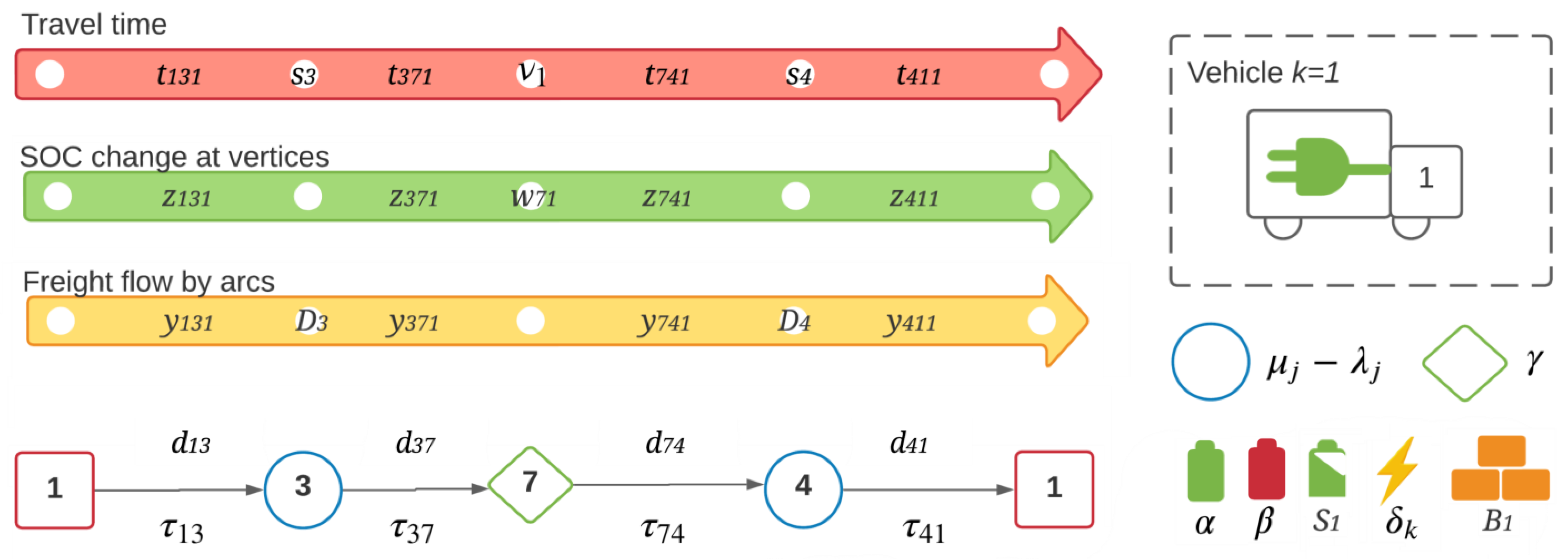
It is necessary to model the dynamics of each of the electric vehicles concerning their travel time, SOC of battery state, and product delivery. Figure 1 illustrates the relationship between the decision variables involved. For the dynamics of travel times $t_{ijk}$, there is an increasing flow of the variable for each vehicle, i.e., each time a vehicle visits a customer departing from the depot, its travel time increases along with the service time $s_j$ characteristic of each customer. The arrival and service times must fit within the customer’s time window $\left[{\lambda }_j,{\mu }_j\right]$. In addition, if the vehicle visits a recharging station, the travel time and the time to recharge the vehicle battery $\gamma$ are added to the total travel time. The figure shows the increased travel time of a vehicle represented by $k=1$ with the red arrow. The vehicle visits the customers located at nodes 3 and 4, and additionally, the vehicle visits the recharging station at node 7. Note that the use of the flow strategy to model the increase in travel time works recursively, similarly to the standard network flow equations.

On the other hand, both the SOC of the battery $z_{ijk}$ and the delivery of goods to customers $y_{ijk}$ have a decreasing flow dynamic. For the case of the SOC, the vehicle begins its route from the depot with the battery at its maximum limit, and the SOC will decrease as it advances along with vehicle visits to the customer nodes. However, the vehicle can recharge its battery, by an amount represented by $w_{ijk}$, by visiting any recharging station. In Figure 1, the green arrow represents the SOC flow for vehicle 1; when it visits node 7, the vehicle is recharging. It is important to note that the SOC should remain between physical battery limits $\alpha , \beta$, and $S_k$.

The modeling strategy also corresponds to a decreasing flow in the delivery of goods. The vehicle will leave the warehouse with a number of goods that does not exceed its capacity on each visit to customers. This load will decrease as it meets the demand of each of the customers. There is no possibility of including goods within the vehicle in the middle of the route. In Figure 1, the yellow arrow represents the flow of goods to customers 3 and 4, who have demands equal to $D_3$ and $D_4$. Finally, the main parameters related to the electric vehicle are in the lower right of Figure 1. In contrast, the parameters of the arcs have been placed accordingly on top of the arrows of vehicle route 1.

2.1. Objective Functions

Four different objective functions are presented in this section: the driven distance, number of required EVs, number of recharging stations, and monetary cost; the objective functions related to the distance driven and cost were taken from [11]. Selecting one of those objective functions gives flexibility in the decision process, allowing for adjustment to meet the desired goal. For instance, a utility firm that offers services in a region may be interested in minimizing the number of vehicles required, to better satisfy its customers or minimize the total costs; thus, the objective function can be chosen accordingly.

The objective function (1) minimizes the total distance driven for a given limit of recharging stations and vehicles.

$$\min f_1={\displaystyle \sum }_{k \in V }{\displaystyle \sum }_{\left(i,j\right) \in A}{d}_{ij}{x}_{ijk}$$

(1)

Furthermore, objective functions (2) and (3) minimize the number of vehicles and recharging stations, respectively. Note that those functions are explicitly written regarding vehicle routing and recharging station-siting decision variables, where $a_j$ represents the recharging station siting.

$$\min f_2={\displaystyle \sum }_{k \in V }{\displaystyle \sum }_{\left(1,j\right) \in A}{x}_{1jk}$$

(2)

$$\min f_3={\displaystyle \sum }_{j \in E}{a}_j$$

(3)

For cases where the monetary cost is the critical function, (4) could be used to minimize the total cost. Within this objective, specific cost factors for investment costs per vehicle $c_k$ [€/day], investments cost per recharging station $c_s$ [€/day], and operational costs $c_d$ [€/day] depending on the distance driven $d_{ij}$ [km] are used.

$$\min f_4=c_k{\displaystyle \sum }_{k \in V }{\displaystyle \sum }_{\left(i,j\right) \in A}{x}_{1jk}+c_s{\displaystyle \sum }_{j \in E}{a}_j+c_d{\displaystyle \sum }_{k \in V }{\displaystyle \sum }_{\left(i,j\right) \in A}{d}_{ij}{x}_{ijk}$$

(4)

Recharging stations are needed when the battery capacity of the vehicles is not enough to complete their routes. Thus, the decision on the optimal allocation depends on the chosen objective function: minimization of the total distance driven, number of vehicles used, number of recharging stations, or total cost. Ultimately, the decision of the optimal allocation depends on the lower bound of the battery capacity.

2.2. Constraints

Based on the formulations of Granada-Echeverri et al. [3] and Toro et al. [37], the proposed model defines a set of constraints (5)–(37). The constraints include the route definition, freight flow by arcs, SOC change at vertices, vehicle traveling times, and nature of the variables.

2.2.1. Route Definition

Constraints (5)–(13) ensure that routes start and end at the depot, with vehicles visiting customers and recharging stations. Equation (5) indicates that all customers must have a single arrival arc, while constraint (6) suggests that the recharging stations should be visited at most once per route, if necessary and if they are available. Note that (5) is written for each customer in set $C$, while (6) is defined by each possible recharging station. The latter establishes that the sum of arc variables for each vehicle $k$ arriving at a recharging station $e$ is at most 1 when the station is built ($a_j$ = 1), or zero otherwise.

Constraint (7) points out that only one vehicle should leave the depot per journey. An arc can also only be used by one vehicle, as indicated in (8). Constraint (9) ensures that, for each vertex $j\in N$, the number of active input arcs must equal the number of active output arcs for each vehicle, i.e., the sum of arcs arriving at node $j$ should be the same as the sum of arcs departing the node. Moreover, (10) and (11) guarantee that the output and the input arcs in the depot are not greater than the number of vehicles in the fleet; note that (10) defines the sum of arcs $\left(1,j\right)$, i.e., leaving the depot, while (11) defines the sum of arcs $\left(i,1\right)$, i.e., arriving the depot when the route is completed. Besides this, for any vehicle $k$, an arc can only be active in one direction, i.e., the sum of the variables related to the arc ($x_{ijk}$ and $x_{jik}$) should be at most 1 when the arc is used, as indicated in (12). Finally, (13) states that the maximum number of arcs traveled by each vehicle $k$ must be less than the number of available arcs.

$${\displaystyle \sum }_{k \in V}{\displaystyle \sum }_{\left(i,j\right)\in A}{x}_{ijk}=1 \forall j\in C$$

(5)

$${\displaystyle \sum }_{k \in V}{\displaystyle \sum }_{\left(i,j\right)\in A}{x}_{ijk}\le a_j \forall j\in E$$

(6)

$${\displaystyle \sum }_{\left(1,j\right)\in A}{x}_{1jk}\le 1 \forall k\in V$$

(7)

$${\displaystyle \sum }_{k \in V}{x}_{ijk}\le 1 \forall \left(i,j\right)\in A$$

(8)

$${\displaystyle \sum }_{\left(i,j\right) \in A}{x}_{ijk}={\displaystyle \sum }_{\left(i,j\right) \in A}{x}_{jik} \forall j\in N, \forall k\in V$$

(9)

$${\displaystyle \sum }_{k \in V}{\displaystyle \sum }_{\left(1,j\right) \in A}{x}_{1jk}\le \left|V\right|$$

(10)

$${\displaystyle \sum }_{k \in V}{\displaystyle \sum }_{\left(i,1\right) \in A}{x}_{i1k}\le \left|V\right|$$

(11)

$${\displaystyle \sum }_{k \in V}{x}_{ijk}+{\displaystyle \sum }_{k \in V}{x}_{jik}\le 1 \forall \left(i,j\right)\in A$$

(12)

$${\displaystyle \sum }_{\left(i,j\right)\in A}{x}_{ijk}\le \left|A\right| \forall k\in V$$

(13)

2.2.2. Freight Flow by Arcs

Constraints (14)–(17) describe the freight flow by arcs, using the variable $y_{ijk}$ to represent the remaining load of vehicle $k$ after traversing arc ($i,j$). As expressed in (14), the flow in the previous vertex $j$ must be equal to the freight flow of the posterior plus the freight demanded by the customer ($D_j$). Constraint (15) indicates that the maximum freight flow per arc cannot be greater than the vehicle freight capacity ($B_k$) and is also limited by the usage of the arc ($x_{ijk}$). Finally, constraint (16) establishes that the freight flow leaving the depot cannot be greater than the depot freight capacity ($b$), while constraint (17) indicates that the freight flow at each recharging station $j$ must be the same at the input and output.

$${\displaystyle \sum }_{k \in V}{\displaystyle \sum }_{\left(i,j\right) \in A}{y}_{ijk}={\displaystyle \sum }_{k \in V}{\displaystyle \sum }_{\left(j,i\right) \in A}{y}_{jik}+D_j \forall j\in C$$

(14)

$$y_{ijk}\le B_k·x_{ijk} \forall \left(i,j\right)\in A, \forall k\in V$$

(15)

$${\displaystyle \sum }_{\left(1,j\right) \in A}{y}_{1jk}\le b \forall k\in V$$

(16)

$${\displaystyle \sum }_{k \in V}{\displaystyle \sum }_{\left(i,j\right) \in A}{y}_{ijk}={\displaystyle \sum }_{k \in V}{\displaystyle \sum }_{\left(j,i\right) \in A}{y}_{jik} \forall j\in E$$

(17)

2.2.3. SOC Update at Vertices

Constraints (18)–(25) define the vehicle battery’s SOC and the operating conditions along the routes by representing the battery energy state of vehicle $k$ after traversing arc ($i,j$) with the variable $z_{ijk}$. Equation (18) allows the calculation of the SOC considering the distance traveled by the vehicle ($d_{ij}$) and its energy consumption rate (${\delta }_k$), while constraint (19) indicates that the SOC in the arcs cannot be greater than the EV battery capacity ($S_k$). When a vehicle leaves the depot, the battery has the maximum SOC level, as guaranteed in (20); that is represented by the sum of the energy states of the vehicle $k$ across the possible arcs leaving the depot (arcs $x_{1jk}$). As also indicated in (21) and (22), the vehicle must have enough SOC to return to the depot or reach a recharging station, i.e., the sum of variables $z_{i1k}$ should be enough to cover the last distance to the depot ($d_{i1}$) along with the lower bound of the battery capacity ($\beta$). Likewise, constraint (23) forces vehicles to leave the recharging stations with a SOC value within the allowable limits (according to parameters $\alpha$ and $\beta$). Constraint (24) establishes that recharging only occurs at vertices with a ready-built recharging station (in which $a_j$ is 1). Finally, constraint (25) limits the number of recharging stations that can be allocated by the number of potential vertices to site recharging stations ($\xi$).

$${\displaystyle \sum }_{k \in V}{\displaystyle \sum }_{\left(i,j\right) \in A}{z}_{ijk}={\displaystyle \sum }_{k \in V}{\displaystyle \sum }_{\left(j,i\right) \in A}{z}_{jik}+{\displaystyle \sum }_{k \in V}{\displaystyle \sum }_{\left(i,j\right) \in A}{\delta }_k·d_{ij}·x_{ijk} \forall j\in C$$

(18)

$$z_{ijk}\le S_k·x_{ijk} \forall \left(i,j\right)\in A, \forall k\in V$$

(19)

$${\displaystyle \sum }_{\left(1,j\right) \in A}{z}_{1jk}=\alpha ·S_k{\displaystyle \sum }_{\left(1,j\right) \in A}{x}_{1jk} \forall k\in V$$

(20)

$${\displaystyle \sum }_{\left(i,1\right) \in A}{z}_{i1k}\ge {\displaystyle \sum }_{\left(i,1\right) \in A}\left(\beta · S_k+{\delta }_k·d_{i1}\right)·x_{i1k} \forall k\in V$$

(21)

$${\displaystyle \sum }_{i \in C_D}{z}_{ijk}\ge {\displaystyle \sum }_{i \in C_D}\left( \beta ·S_k+{\delta }_k·d_{ij}\right)·x_{ijk} \forall j\in E, \forall k\in V$$

(22)

$$\beta ·S_k{\displaystyle \sum }_{j \in C_D}{x}_{ijk}\le {\displaystyle \sum }_{j \in C_D}{z}_{ijk}\le \alpha ·S_k{\displaystyle \sum }_{j \in C_D}{x}_{ijk} \forall i\in E, \forall k\in V$$

(23)

$$z_{ijk}\le S_k·a_j \forall i\in C_D, \forall j\in E, \forall k\in V$$

(24)

$${\displaystyle \sum }_{j \in E}{a}_j\le \xi$$

(25)

2.2.4. Traveling Times

Constraints (26)–(31) describe the arrival time of each vehicle in the route, considering customer service and the recharging time required at stations; variable $t_{ijk}$ is used to represent the time of arrival at vertex $j$, from vertex $i$, for vehicle $k$, and parameter ${\tau }_{ij}$ corresponds to the traveling time between vertices $i$ and $j$. The total arrival time represents the time required to visit the last customer on the route. Thus, constraint (26) describes the arrival time for each customer bearing in mind their service time $s_j$ [min.], by setting the time to arrive at the next vertex $i$ ($t_{jik}$) in terms of the time when the vehicle arrived at vertex $j$ ($t_{ijk}$), along with the travel time and service time (${\tau }_{ij}$ and $s_j$).

Since the customer must be visited within a time window, constraints (27) and (28) limit the time intervals, considering the earliest and latest times of allowed arrival (${\lambda }_j$ and ${\mu }_j$). On the other hand, constraint (29), similar to (26), is applied at recharging stations to calculate the arrival time as well as the recharging time $w_{jk}$ [min.]. Constraint (30) describes how the SOC of vehicle $k$ changes at the recharging station considering the recharging rate ${\sigma }_k$ [W] and recharging time $w_{jk}$. Likewise, this recharging time is limited to ensure that the vehicle does not remain at the recharging station, as specified by (31) and considering the upper bound for the recharging time at a recharging station ($\gamma$).

$${\displaystyle \sum }_{k \in V}{\displaystyle \sum }_{\left(i,j\right) \in A}{t}_{jik}={\displaystyle \sum }_{k \in V}{\displaystyle \sum }_{\left(i,j\right) \in A}{t}_{ijk}+{\displaystyle \sum }_{k \in V}{\displaystyle \sum }_{\left(i,j\right) \in A}\left({\tau }_{ij}+s_j\right)·x_{ijk} \forall j\in C$$

(26)

$$t_{ijk}\le \left({\mu }_j+s_j\right)·x_{ijk} \forall \left(i,j\right)\in A, \forall k\in V$$

(27)

$$t_{ijk}\ge {\lambda }_j·x_{ijk} \forall \left(i,j\right)\in A, \forall k\in V$$

(28)

$${\displaystyle \sum }_{k \in V}{\displaystyle \sum }_{\left(i,j\right) \in A}{t}_{jik}={\displaystyle \sum }_{k \in V}{\displaystyle \sum }_{\left(i,j\right) \in A}{t}_{ijk}+{\displaystyle \sum }_{k \in V}{\displaystyle \sum }_{\left(i,j\right) \in A}\left({\tau }_{ij}+s_j\right) x_{ijk}+{\displaystyle \sum }_{k \in V}{w}_{jk} \forall j\in E$$

(29)

$${\displaystyle \sum }_{\left(i,j\right) \in A}{z}_{ijk}+{\sigma }_k\cdot w_{jk}={\displaystyle \sum }_{\left(i,j\right) \in A}{z}_{jik}+{\displaystyle \sum }_{\left(i,j\right) \in A}{\delta }_k·d_{ij}·x_{ijk} \forall j\in E, \forall k\in V$$

(30)

$$w_{jk}\le \gamma ·a_j\forall j\in E, \forall k\in V$$

(31)

2.2.5. Nature of Variables

The nature of the variables in the problem is defined by (32)–(37). The binary nature of variables $a_j$ and $x_{ijk}$ is defined by (32) and (33), respectively. The continuous nature of the variables that describe the time, such as $t_{ijk}$ and $w_{jk}$, is defined by (34) and (35), respectively; similarly, (36) and (37) represent the continuous nature of variables $y_{ijk}$ and $z_{ijk}$, respectively. Overall, model (1)–(37) is a MILP formulation that can be implemented in a mathematical modeling language and solved using commercial solvers.

$$a_j\in \left\{0,1\right\} \forall j\in E$$

(32)

$$x_{ijk}\in \left\{0,1\right\} \forall \left(i,j\right)\in A, \forall k\in V$$

(33)

$$t_{ijk}\in {ℝ}^{+} \forall \left(i,j\right)\in A, \forall k\in V$$

(34)

$$w_{jk}\in {ℝ}^{+} \forall j\in E, \forall k\in V$$

(35)

$$y_{ijk}\in {ℝ}^{+} \forall \left(i,j\right)\in A, \forall k\in V$$

(36)

$$z_{ijk}\in {ℝ}^{+} \forall \left(i,j\right)\in A, \forall k\in V$$

(37)

3. K-Means Algorithm

The k-means algorithm is used in this section to classify data using patterns that may exist in a database [38]. This process includes identifying similar data in the same set and adding a label representing a category [39].

MacQueen created this algorithm in 1967 for simple unsupervised learning to solve a clustering problem [40]; its classification method finds a local minimum through the convergence of an iterative process in the assignment of groups until they are independent and compact. Its application is extensive, fast, simple, and effective in producing data clusters in fields like biology and medicine, including artificial intelligence and data mining [39].

K-means consists of two separate phases. The first phase randomly defines the centroids, while the second phase assigns each datum to the nearest centroid according to the Euclidean distance. The initial clustering corresponds to that first association between centroids and data. This process is carried out until the function criterion (e.g., distance) reaches the minimum [39]. Figure 2 shows in detail the clustering process performed by the k-means algorithm.

3.1. Recharging Station Assignment

The k-means algorithm adopted in this work is based on the proposal by [41]. It is assumed that there is a data set $H=\left\{h_1,\dots ,h_L\right\}$, $h_l\in {ℝ}^2$. The objective is to divide the data into $m$ groups $F_1,\dots ,F_m$ until the clustering criterion is optimized. It is worth highlighting that $m$ is the parameter previously defined. The most used clustering criterion is the sum of the square Euclidean distances between each data point $h_l$ and its related centroid $M_p$, within cluster $F_p$. This criterion is called the cluster error criterion and depends on the $M_1,\dots ,M_m$ centroids, as defined by (38).

$$\epsilon \left(M_1,\dots ,M_m\right)={\displaystyle \sum }_{l=1}^L{\displaystyle \sum }_{p=1| l \in F_p}^m\Vert h_l-M_p\Vert$$

(38)

The k-means algorithm randomly places the centroids and then moves them at each stage to minimize the error. The disadvantage of that process lies in the sensitivity of the starting positions, given their random selection; it is known that cluster performance error depends on the initial starting conditions [42]. Moreover, the process is deterministic, depending solely on the number of clusters as the input parameter. Some authors have considered metaheuristics such as GA or multiple restarts to solve this problem [43]. Further authors have presented research seeking to improve the efficiency of the technique, such as the k-means algorithm based on weights [44], which assigns loads to the numeric and symbolic attributes of the data, thus significantly reducing noise and the effect data without a characteristic pattern. Yet, the downside is that it takes longer to execute. Other studies have proposed solving data clustering systematically to find initial centroids of the sets that are consistent with the data distribution, thus obtaining more accurate results than with the traditional algorithm; however, the execution time and complexity are greater (Yuan 2004). Some works have aimed to improve the solution time, considering that even if the results are the same as with the standard algorithm, the speed of clustering and its complexity are enhanced [39].

In the proposed method, the k-mean algorithm defines vertices where the recharging stations can be located and the customer’s area. Hence, each centroid of the algorithm represents a possible localization for a charging station while each cluster represents a customer’s area. That information is part of the input for the formulation, as presented in Section 2. A graphical description is shown in Figure 3, where two example clusters are defined; in green, customers are related to the cluster on the left, while customers in blue are related to the cluster on the right. According to Algorithm 1, the strategy begins by obtaining the database containing the customer location and depot. Then, the user determines the number of groups and inserts them into the k-means algorithm. Subsequently, the centroids are calculated, labeled, and stored. The calculation of the centroids generates a new vertex with its respective coordinates. Likewise, each datum has a color assigned corresponding to its respective customer’s area. Then, new vertices containing the centroids’ coordinates and the recharging stations are added to the database.

3.2. Strategies for Search Space Reduction

Additional constraints are imposed to reduce the computational effort. It is assumed that visiting two charging stations one after the other is unnecessary. Therefore, constraint (39) is added to the model to forbid the use of direct arcs between recharging stations. Since the depot serves as a recharging station, the EVs leave with their batteries at full capacity. Thus, a visit to a recharging station directly after leaving the depot is not necessary, as indicated by (40).

Algorithm 1. Assignment process of new vertices in the database

Input $p:$ Number of clusters $C_D:$ Set of customers including depot vertex Output $N:$ Set of vertices including recharging stations and depot vertex $C_D\leftarrow obtain\_data()$  $kmeans\leftarrow kmeans\_algorithm\left(p\right)$  $label\leftarrow kmeans.predict\left(X\right)$  $centroids\leftarrow kmeans.cluster\_centroid\_$ For line in label do       $assignment\leftarrow color\left(line\right)$ End For m in (1, …, p + 1) do      $potential\leftarrow C_D+centroids$ End  $N\leftarrow optimization\_site\left(potential\right)$

$$x_{ijk}=0 \forall k\in V, \forall i\in E, \forall j\in E, i\ne j$$

(39)

$$x_{1jk}=0 \forall k\in V, \forall j\in E$$

(40)

The information obtained with the k-means algorithm serves to group customers, identify centroids, and reduce the variables in the mathematical model. In a real context, the number of customers can be large and exact algorithms may not achieve excellent computational performance. Consequently, and to address this shortcoming, companies divide their customer into operation areas and assign certain fleet vehicles to each one. That strategy provides good-quality solutions under a reasonable computational effort. Therefore, the main idea of using k-means is to mimic that common company practice.

Additionally, and to avoid overlapping, arcs between different clusters are avoided, as indicated in constraint (41). This offers a significant advantage in computation time, while having a limited impact on the solution quality.

$$x_{ijk}=0 \forall k\in V, \forall i\in F, \forall j\in F, i\ne j$$

(41)

4. Case Study

Performed experiments are based on the modified Solomon instances presented by [11] and allow for analysis of how the location of recharging stations influences the routing solution. The design of the experiments is described in this section. The advantages of the mathematical formulation proposed in Section 2, recharging station-siting decisions described in Section 3, and impact of the different objective functions are shown here.

Solomon instances are constituted by vehicles with a homogeneous freight capacity of 200 units, and consist of three groups named C, R, and RC. These groups are divided into two subgroups each: C1, C2, R1, R2, RC1, and RC2. Those instances were created by considering several factors that affect the routing and planning algorithms’ behavior, such as geographical data, the number of customers served per vehicle, and the percentage of customers with time windows. In problems R1 and R2, the geographic data are randomly generated, while problems C1 and C2 are grouped or clustered. Finally, problems RC1 and RC2 are a mixture of random and grouped structures. The coordinates of two customers are identical in each group, with the differences in the time windows. The original Solomon problems have 100 customers, and the traveling times correspond to Euclidian distances.

To introduce recharging station planning, Dominik et al. [12] generated instances by taking the information of [11] but reducing the numbers of customers to 5, 10, and 15. These instances are identified using Solomon’s original nomenclature as the number of customers for Dominik’s instances. In this way, a case of a study named RC203-5 was generated using the original Solomon dataset RC203, using information for five customers to create Dominik’s dataset. The first possible recharging substation location was the depot, marked as vertex one. Other possible recharging station locations were decided in a way that guaranteed every customer could be reached from the depot by using at most two recharging stations. Finally, all customers had to be reached in a feasible time.

The experiments in this paper used the customer information from [12], and the possible locations of the recharging stations were determined by the centroid generated for the k-means algorithm. Complete information on the possible vertices of the recharging stations for the 24 test instances is available in [45]. For comparison purposes,

Table 2. Characteristics of the new potential vertices for the locations of recharging stations in each Dominik and Schneider’s instance generated by the k-means algorithm.

Instance	j	${\mathit{X}}_{\mathit{j}}$	${\mathit{Y}}_{\mathit{j}}$	${\mathit{D}}_{\mathit{j}}$	${\mathit{\lambda }}_{\mathit{j}}$	${\mathit{\mu }}_{\mathit{j}}$	${\mathit{s}}_{\mathit{j}}$
C101-5	1	44.0	40.0	0.0	0.0	1236.0	0.0
	2	22.5	70.0	0.0	0.0	1236.0	0.0
	3	61.5	72.5	0.0	0.0	1236.0	0.0
R104-5	1	21.0	24.7	0.0	0.0	230.0	0.0
	2	57.0	68.0	0.0	0.0	230.0	0.0
	3	38.0	42.0	0.0	0.0	230.0	0.0
RC208-5	1	45.3	47.0	0.0	0.0	960.0	0.0
	2	87.0	30.0	0.0	0.0	960.0	0.0
	3	61.5	78.5	0.0	0.0	960.0	0.0

j = index of recharging station; X = horizontal coordinate; Y = vertical coordinate; $D_j$ = demand of vertex [units]; ${\lambda }_j$ = earliest time of arrival allowed at vertex [min]; ${\mu }_j$ = latest time of arrival allowed at vertex [min]; $s_j$ = service time at vertex [min].

illustrates the parameters of the potential recharging stations when sited for Dominik et al. instances.

5. Results

The mathematical model described in Section 2 was implemented in AMPL [46] and solved via CPLEX version 20.1 [47]. The simulations were executed using a computer with an Intel Xeon Silver 4116 processor and 128 GB of RAM within a Python 3.8 environment. The time limit for solving the instances was set to 7200 s.

All cases were evaluated considering a single depot. Besides this, the EV freight load capacity $B$ = 200 units with an EV fleet of $V$ = 5, the freight load capacity at the depot vertex $b$ = 500 units, and the battery capacity $S_k$ = 30 kWh. The energy consumption per kilometer traveled ${\delta }_k$ = 200 Wh/km, and the average speed per vehicle $v_k$ = 1 km/min, while the recharge rate of the batteries ${\sigma }_k$ = 12 kW. The upper charging time limit at the recharging station $\gamma$ = 120 min. Cost coefficients were derived for a real-world case study of a mid-haul logistic network [26]; these were calculated in euros per day and were fixed as $c_d$ = 0.0508 €km⁻¹/day, $c_k$ = 53.32 €/day, and $c_s$ = 2.47 €/day. To prevent the battery from being completely drained or fully charged, to maintain its lifespan, $\alpha$ = 0.8 and $\beta$ = 0.2 were defined [48], ensuring that the SOC of each vehicle was between 20% and 80% of its capacity when leaving the depot and recharging stations.

The detailed results for all cases are shown in

Table 3. Results for the ELRP-TWPR.

Instance	Objective 1					Objective 2					Objective 3					Objective 4
	v	d	c	s	t	v	d	c	s	t	v	d	c	s	t	v	d	c	s	t
C101-5	3	280.9	181.5	3	2.14	3	280.9	181.5	3	2.50	3	280.9	18159	3	1.24	3	280.9	181.5	3	3.42
C103-5	2	169.1	117.7	1	0.95	2	189.6	121.1	2	1.28	2	169.1	117.7	1	0.41	2	169.1	117.7	1	1.39
C206-5	2	262.1	124.8	2	3.33	1	349.3	80.7	4	2.38	2	262.1	124.8	2	0.55	1	348.3	78.3	3	1.01
C208-5	2	252.5	124.3	2	2.31	2	315.5	129.9	3	3.84	3	282.6	179.2	2	1.41	2	252.5	124.3	2	4.67
R104-5	2	165.4	117.5	1	1.69	2	203.9	124.3	3	0.42	2	165.4	117.5	1	0.63	2	165.4	117.5	1	1.84
R105-5	2	168.5	120.0	2	1.73	2	212.1	124.7	3	0.64	3	240.3	177.0	2	1.16	2	168.5	120.0	2	2.56
R202-5	1	178.2	67.2	2	0.64	1	192.4	67.9	2	1.47	3	246.2	174.9	1	0.30	1	178.2	67.21	2	2.31
R203-5	1	194.2	70.4	3	1.22	1	224.5	71.9	3	0.20	2	240.7	121.3	1	0.47	1	196.3	68.1	2	3.81
RC105-5	2	217.9	125.0	3	1.97	2	217.9	125.0	3	2.19	3	274.9	178.8	2	1.91	2	217.9	125.0	3	2.67
RC108-5	2	248.8	126.5	3	3.45	2	266.4	129.8	4	2.13	3	372.3	186.1	3	0.80	2	248.8	126.5	3	6.77
RC204-5	2	178.0	120.5	2	1.00	1	276.2	74.6	3	0.44	3	265.4	178.3	2	1.73	1	179.0	69.7	3	1.84
RC208-5	1	172.4	66.9	2	1.95	1	220.5	69.4	2	2.84	2	211.3	117.4	0	1.39	1	172.4	66.9	2	4.61
C101-10	5	701.3	314.0	5	14.1	5	710.5	314.8	5	32.6	5	743.3	316.5	5	35.4	5	701.3	314.3	5	305.6
C104-10	3	354.6	182.8	2	5.0	3	387.2	189.3	4	7.75	4	431.3	240.0	2	4.06	3	354.6	182.8	2	12.19
C202-10	5	536.6	306.0	5	77.9	5	552.7	306.8	5	7.98	5	551.7	304.3	4	14.9	5	543.4	303.9	4	16.78
C205-10	5	505.9	297.1	2	4.27	4	513.0	246.6	3	12.75	5	505.9	297.1	2	6.02	4	508.3	246.4	3	8.42
R102-10	5	429.6	295.7	3	3.36	5	473.2	300.3	4	5.50	5	481.0	298.3	3	2.91	5	429.6	295.7	3	5.61
R103-10	2	207.0	119.6	1	1.24	2	210.9	124.6	3	1.19	4	290.0	230.4	1	0.44	2	207.0	119.6	1	2.06
R201-10	4	340.0	237.8	2	4.22	4	397.7	243.2	4	6.20	5	389.4	293.7	3	2.98	4	340.0	237.8	3	3.14
R203-10	2	306.6	131.9	4	3.80	2	480.3	143.1	5	1.97	5	370.3	290.3	2	2.75	2	306.6	131.9	4	38.11
RC102-10	4	497.6	245.8	3	4.11	4	498.6	248.3	4	4.02	5	548.1	301.7	3	4.83	4	497.6	245.8	3	4.08
RC108-10	4	447.0	243.2	3	4.28	4	481.4	247.4	4	3.03	4	447.1	240.8	2	4.28	4	447.1	240.8	2	2.92
RC201-10	5	476.9	300.5	4	5.08	4	558.4	251.3	4	7.09	4	488.6	242.9	2	2.67	4	488.6	242.9	2	6.38
RC205-10	5	529.0	300.7	3		5	571.9	305.3	4	6.81	5	552.3	301.9	3	4.64	5	529.0	300.7	3	6.72

v = number of used vehicles; d = overall traveled distance [km]; c = overall costs [€/day]; s = number of different recharging stations used; t = computational time [s]; g = gap between found solution and the best lower bound [%].

, including information about the four objective functions described in Section 2. The results show that the model can find the optimal solution, i.e., the solution gap was 0% for all instances. It is worth highlighting that the computation times for Objective 4 ($f_4$) are higher than those for the other objective functions in most instances. This can be justified by the combined optimization of the distance and number of EVs/recharging stations under $f_4$, which requires more effort to optimize the routes, rather than finding just the minimum number of EVs ($f_2$) or recharging stations ($f_3$).

When the instances are solved minimizing Objective 2, the number of vehicles in the planned fleet is smaller than the minimization of Objective 3. At the same time, there is an inverse relationship between the number of vehicles and the number of recharging stations; when comparing the results obtained using Objectives 2 and 3, for instance, the former has a larger number of recharging stations than the latter. As an illustration, consider the results of R105-5, where two EVs and three recharging stations are needed when Objective 2 is minimized. In comparison, three EVs and two charging stations are required when Objective 3 is minimized. Hence, Objectives 1 and 4 show the best results related to the distance traveled, total cost, number of vehicles, and charging stations. In some cases, Objective 4 shows a subtle difference when compared to the optimal solution achieved by Objective 1.

The clustering technique adopted can allow cases to be solved with more customers and still have a reasonable quality of solution. The clustering technique used in Section 3 reduces the search space, leading to low computational times even if the number of vertices increases. To illustrate this, if instance R203-10 is solved to minimize Objective 4 without using k-means, the value of the objective function coincides with that obtained by applying the clustering algorithm, but the computational time spent is 2.245 s; this corresponds to an increase of 5.790% when compared to the result shown in Table 3. It is important to point out that the computational times are presented to show the competitiveness of the modeling and implementation developed for the planning problem, without it being the main interest when solving this kind of problem.

Figure 4 shows a compilation of the optimal routes obtained for each objective function for the R105-5 instance, with a fleet of five EVs and three potential vertices for recharging stations. Figure 4a shows the optimal route for Objective 1, in which two EVs are used to visit all customers; two recharging stations are built and utilized by each EV only once on their routes. For Objective 2, two EVs are used to visit all customers, and three recharging stations are built; vehicle 5 visits two recharging stations, while vehicle 4 visits only one, as shown in Figure 4b.

Figure 4c shows the optimal routes for Objective 3, in which three EVs are used to visit all customers and two recharging stations are proposed. Objective 4 obtained the same route solution as Objective 1, including the siting of recharging stations. The variation is that different EVs leave the depot, as shown in Figure 4d; this is possible because the fleet is homogeneous in terms of freight and price; in the case of a heterogeneous fleet, the same EVs would be used, but in this situation, the choice of EVs would not affect the objective function. Objectives 1 and 4 obtained the minimum distance and total cost for that customer distribution. In contrast, Objectives 2 and 3 had the worst values since a different charging station or longer vehicle route was needed, respectively.

6. Conclusions

The electric location routing problem with time windows (E-LRPTW) is a complex optimization problem that seeks to minimize the transport costs associated with freight delivery routes considering the limitations inherent to the autonomy of electric vehicles (EVs). Thus, it is necessary todevelop models that find global solutions to this problem in different operational situations of transport logistics.

A mixed-integer linear programming model (MILP) has been proposed for the E-LRPTW, considering siting of recharging stations, in which fleet characteristics are considered in the model. Moreover, the proposed model can minimize different objective functions. As a salient aspect, a clustering strategy was adopted to mimic the real-world logistic companies’ strategies to reduce computational effort. The model was implemented in the mathematical modeling language AMPL and solved via the commercial solver CPLEX. The MILP achieved the optimal solutions for all simulated scenarios. The clustering strategy with k-means contributed to finding the optimal locations for charging stations and reducing the binary variables and computational effort.

Results showed that the number of EVs is mainly defined by the freight demand and customer time windows. The recharging station position, time windows, and EV battery capacity impact the visits and their order. Minimizing the number of EVs and recharging stations increased the traveled distance. It was observed a correlation between EVs and recharging stations, whereby minimizing the number of EVs increases the number of recharging stations. Optimizing the number of charging stations built in a set of potential vertices helps to support optimal routes that minimize EV routing costs. The number of charging stations is reduced when construction costs are considered. These stations can be sited at customer locations or in the middle of routes in the model.

Some simplifications were made in the development of the formulation, namely: (1) the queuing time at the recharging station was disregarded; (2) the EVs’ velocity between vertices was deemed constant, and the road slope was disregarded; (3) the energy consumption rate was considered a linear function depending on the distance driven; and (4) the recharging time at stations depended linearly on the amount of energy consumed.

Information related to EVs is deterministic. The model incorporates EVs’ travel time and their batteries’ state of charge. The travel time is influenced by the distance between customers, their service times, and customer time windows, and these parameters are deterministic. EVs’ recharging time and the battery charge’s spent rate have been considered parameters that do not change over time.

Overall, the results show that simultaneous routing and siting optimization for the E-LRPTW with an efficient clustering strategy to divide customers into areas reduces the computational effort. As this paper shows, the outcomes can be extended to heterogeneous or mixed fleets for even different approaches to solving the E-VRP. Future research may be carried out on real-world instances spanning larger geographical regions, including challenging traffic constraints of the major cities, with higher numbers of recharging stations, and integrating specific cases for the planning of logistics companies.