Abnormal Data Detection and Identification Method of Distribution Internet of Things Monitoring Terminal Based on Spatiotemporal Correlation

Abstract

As an important part of the ubiquitous power Internet of Things, the distribution Internet of Things can further improve the automation and informatization level of the distribution network. The reliability of the measurement data of the low-voltage terminal unit, as the sensing unit of the sensing layer of the distribution Internet of Things, has a great impact on the fault processing and advanced applications of the distribution Internet of Things. The self-check and the equipment working status monitoring of the main station of the low-voltage terminal unit struggle to identify the abnormality of measurement data. Aiming at this problem, an abnormal data detection and identification recognition method of a distribution Internet of Things monitoring terminal is proposed on the basis of spatiotemporal correlation. First, using the temporal correlation of monitoring terminal data, the proposed composite temporal series similarity measurement criterion is used to calculate the distance matrix between data, and the abnormal data detection is realized via combination with the improved DBSCAN algorithm. Then, using the spatial correlation of the data of the terminal unit, the geometric features of the spatial cross-correlation coefficient of the terminal nodes are extracted as the input of the cascaded fuzzy logic system to identify the abnormal source. Lastly, the effectiveness of the method is verified by a practical example.

1. Introduction

As an important part of the ubiquitous power Internet of Things, the distribution Internet of Things can effectively improve the automation and informatization level of the distribution network [1,2] and provide users with diversified and differentiated energy services; thus, further enhancing the level of electricity safety for customers [3,4]. The architecture of the distribution Internet of Things is divided into a perception layer, a network layer, a platform layer, and an application layer. The perception layer is located at the end of the distribution Internet of Things, and it can transmit the information collected by a large number of low-voltage terminal units (LTUs) in the distribution network to the application layer through the network layer, providing data support for the functions of fault detection and low-voltage load monitoring in the distribution Internet of Things [5]. Data analysis or decision making at the application layer need to ensure the quality of the data. The measurement data collected and sent by the LTU may be abnormal due to various reasons. Generally speaking, data anomalies can be divided into two categories. One category involves data interruption or data anomalies caused by problems such as communication module failure, battery energy exhaustion, and sampling circuit failure in the LTU, which can be detected through the self-checking of the LTU or equipment working status monitoring of the master station. The second category involves data abnormalities caused by sampling circuit failure and abnormal storage modules that cannot be detected by the LTU equipment; such data may only have a small step on the basis of normal data, and these abnormalities are difficult to detect through the self-checking of the LTU or equipment working status monitoring of the master station. Due to the characteristics of the many points, wide areas, and large numbers of LTUs, it is difficult to detect in time when an abnormality occurs. False alarms or omissions of faulty LTUs may affect the accuracy and reliability of system troubleshooting and advanced applications; therefore, it is an important part of improving the operation reliability of the distribution Internet of Things system and the management level of the system equipment to perform abnormal detection on the measurement data of the LTU, find the abnormal data, and confirm its source.

At present, there are few studies on the detection of abnormal data of LTUs in the distribution Internet of Things, but there are many abnormal data detection methods for IoT terminals, which can be divided into four categories: (1) anomaly detection methods based on statistics [6,7], which need to establish a complete dataset in advance and understand the prior information, resulting in limited detection conditions and poor real-time performance; (2) distance-based anomaly detection methods [8,9] for detecting the top n outliers based on the distance function; however, this method increases the network communication overhead and is not suitable for dynamic changes in network topology and multidimensional data; (3) density-based anomaly detection methods [10,11], which take a long time to calculate; if the size of the dataset is m, the time complexity is O(m²), making this method unsuitable for the detection of power distribution IoT data with a large amount of data requiring real-time monitoring; (4) anomaly detection methods based on pattern recognition [12,13]. Due to the nonlinearity, complexity, ambiguity, and randomness of abnormal data during the operation of LTUs, it is difficult to express with precise mathematical equations, and the complex working environment of LTUs puts forward higher requirements for the real-time performance and robustness of the detection method. The pattern recognition method is a better method to solve this kind of problem. Some scholars used Bayesian networks [14,15], neural networks [16,17], and other methods to establish a prediction model from historical timeseries data. Such methods require known prior probabilities, and the detection effect is directly related to the setting of the deviation threshold. The authors of [18] proposed a global outlier detection method based on clustering. Cluster-based methods do not require prior knowledge of the data distribution and can use incremental models, which provide the system with new data instances and perform outlier detection.

There are few related studies on the identification of IoT abnormal data sources. The authors of [19] used the median of historical data to establish pivot quantities, and abnormal data source discrimination was realized by calculating the degree of difference between data intervals. The authors of [20] used the Markov chain to extract the spatiotemporal features of IoT sensor data streams on the basis of the spatiotemporal correlation of IoT data, which were then used as input features for a multiclass CNN model to identify abnormal sources. However, this method requires the offline training of the multiclass CNN model using datasets with various abnormal labels in advance. The above two methods ignore the time correlation, resulting in a limited measurement accuracy.

Aiming at the problem of abnormal data detection, this paper proposes an abnormal detection and identification method of LTU nodes in the distribution Internet of Things. The method can be divided into two parts.

The first part is the cluster-based LTU anomaly detection method. First, in view of the problem that the traditional similarity measurement method has a poor effect on the similarity measurement of high-dimensional data, using the temporal correlation of LTU measurement data and considering the local similarity and global similarity of the measurement sequence, an improved composite timeseries similarity measure is proposed, which can improve the accuracy of the input data during the cluster analysis. Then, in order to overcome the problem that the traditional DBSCAN algorithm is sensitive to the selection of clustering parameters, a DBSCAN algorithm for adaptively generating clustering parameters is proposed, thereby obtaining the core data points representing the change characteristics of the measurement data through clustering training, before calculating the relationship between the distance between the real-time measurement data and the core data points and the neighborhood radius Eps through a composite timeseries similarity measure. The comparison of real simulation results in Section 5.4.1 shows that the improved DBSCAN algorithm has a lower false alarm rate and higher practical value when the detection rate is higher.

The second part is the anomaly source detection based on a fuzzy logic system. The first part realizes the detection of abnormal data, whereas this part uses the spatial correlation of the LTU measurement data of the distribution Internet of Things to distinguish the abnormal data from line events or LTU faults. First of all, using the spatial correlation of the distribution Internet of Things data, the sliding time window algorithm is used to calculate the spatial cross-correlation coefficient between the LTU with abnormal data and its neighboring LTUs, while the geometric features of the spatial cross-correlation coefficient are extracted as the input of the fuzzy logic system. Then, in view of the problem that it is difficult to obtain the evaluation of the spatial correlation of nodes through a certain quantitative calculation equation, a fuzzy logic algorithm that can process imprecise information based on the fuzzy set theory is selected and combined with the spatial and temporal correlation of the data of the distribution Internet of Things. Accordingly, a cascaded fuzzy logic system is designed to evaluate the spatial correlation between LTUs, by evaluating the degree of spatial correlation between the abnormal data LTU and its neighboring devices, allowing it to distinguish whether the abnormal data come from line events or LTU failures.

2. Cluster-Based LTU Anomaly Detection Method

2.1. Source of Abnormal State of LTU in Low-Voltage Distribution Network

The causes of abnormal data generated by the LTU mainly include the following types of faults:

①

Hardware faults: Hardware faults are mostly caused by the failure of the internal communication module of the LTU, the exhaustion of battery power, or the failure of some types of A/D conversion modules. Measurement data usually show data interruption or measurement data at a positive/negative limit.

②

Stuck-at faults: Stuck-at faults are characterized by a series of offset and continuous readings, and these sampling data may persist in subsequent sampling cycles. The offset is maintained or may return to normal after a period of time. The offset sampling data may be within the normal sampling data range or may exceed the range of the normal sampling data. Such faults are generally caused by the abnormality of the internal sampling module of the LTU.

③

Low-voltage faults: Typical low-voltage faults usually manifest as a result of constant sampling data or offset values, which significantly increase the data noise. This type of fault is generally caused by an abnormal drop in battery power due to an internal/external short-circuit of the battery when the LTU is in battery power supply mode.

④

Calibration failure: The reason for this failure is a calibration error, which is manifested as a relatively fixed offset between the sampled data and the actual data, which may be large or small.

The abnormal data generated by type ① faults can be detected more accurately by the self-check of the LTU and the equipment working status monitoring of the master station, whereas the abnormal data of types ②, ③, and ④ may only have a small step on the basis of normal data; thus, it is difficult to detect and monitor the working state of the equipment. This paper mainly detects these three types of abnormal data.

2.2. Anomaly Detection Method Based on Clustering

2.2.1. Improved Composite Timeseries Similarity Measure

The measurement data of LTUs in the distribution Internet of Things involve typical timeseries data. For two given LTU nodes, Ω_i and Ω_j, the measurement sequence aggregated every m minutes until the time instant t could be expressed as shown in Equation (1).

$$\begin{array}{l}{F}_i=\left\{f_{i,1},f_{i,2},\dots ,f_{i,t}\right\},\\ F_j=\left\{f_{j,1},f_{j,2},\dots ,f_{j,t}\right\}\end{array}$$

(1)

where F_i and F_j are the univariate observation timeseries of LTUs, and f_i,t and f_j,t are the corresponding data points.

First, in order to understand the statistical structure of the LTU datasets, a composite timeseries similarity measure was defined to measure the similarity between the output data from two LTUs. The Euclidean distance is the most used in similarity measurements between data, but it has a poor effect on the similarity measurement of high-dimensional data and is not a comprehensive distance measurement method. Therefore, a composite timeseries similarity measure matrix D = {d_i,j}_n×n was proposed in this paper, where d_i,j is composed of three distances as shown in Equation (2).

$$d_{i,j}=\frac{1}{2}{d}_{{}_{i,j}}^{\cos }+\frac{1}{4}{d}_{{}_{i,j}}^{\mathrm{jsd}}+\frac{1}{2}{d}_{{}_{i,j}}^{\mathrm{mis}}.$$

(2)

Distances d^cos, d^jsd, and d^mis are defined as shown in Equations (3)–(5).

$$d_{{}_{i,j}}^{\cos }=1-\cos (F_{{\Omega }_{i,t}},F_{{\Omega }_{j,t}})=1-\frac{F_{{\Omega }_{i,t}}•F_{{\Omega }_{j,t}}}{‖F_{{\Omega }_{i,t}}‖•‖F_{{\Omega }_{j,t}}‖},$$

(3)

$$\begin{array}{l}{d}_{\mathrm{K}L}(P_i\parallel P_j)={\displaystyle \sum _i{p}_i(f)\ln \frac{p_i(f)}{p_j(f)}}\\ M=\frac{1}{2}(P_i+P_j),\\ d_{{}_{i,j}}^{\mathrm{jsd}}=\frac{1}{2}{d}_{\mathrm{KL}}(P_i\parallel M)+\frac{1}{2}{d}_{\mathrm{KL}}(P_j\parallel M)\end{array}$$

(4)

$$\begin{array}{l}{\phi }_i=\left\{\begin{array}{l}1,if\exists x\in \left\{1,\dots t\right\},f_{i,x}<0\vee f_{i,x}=NaN\\ 0,\hspace{0.17em}otherwise,\end{array}\right.\\ D_{{}_{i,j}}^{\mathrm{mis}}=\left\{\begin{array}{l}0,if{\phi }_i={\phi }_j\\ 1,\mathrm{otherwise}\end{array}\right.\end{array}$$

(5)

where d^cos is the cosine similarity, which is different from the Euclidean distance; it needs to reflect the difference in the size of the value and it is suitable for high-dimensional data. d^jsd is calculated by the JS divergence (Jensen–Shannon), which represents the similarity of the probability density distribution between two sequences F_i and F_j. d^mis is the error mode distance, which represents whether F_i and F_j have or do not have missing values in the sampled data stream or have data less than 0, where P_i = p_i(f) is the probability density function obtained by estimating the kernel density of the Ω_i data sequence.

The improved composite timeseries similarity measure proposed in this paper comprehensively measures the similarity of LTU timeseries from three aspects—the amplitude, probability distribution, and error mode, making it suitable for mining timeseries data from the distribution Internet of Things; thus, providing an accurate information input for the cluster analysis as described later. The error mode distance was calculated using the data stream without data padding, whereas the Euclidean distance and JS divergence were calculated using the data stream after data cleaning.

Then, the distance matrix calculated from the preprocessed LTU historical measurement data was used as an input to cluster the LTU measurement data. The specific preprocessing method is given in Section 5.1. In this paper, a density-based spatial clustering of applications with the noise (DBSCAN) algorithm was used to cluster the LTU node data. DBSCAN is a typical density-based clustering algorithm, which can distinguish data into boundary points, core points, and noise points according to the tightness of the data distribution. It has the following characteristics:

• The calculation speed is fast and can be used for larger datasets;
• It can find classes of any shape in the dataset;
• The clustering effect is better when the density gap between various types is small.

Distribution IoT data have the characteristics of a large quantity, compact spatial distribution, and high density, while abnormal data distribution is discrete and the proportion of data volume in the dataset is very low; hence, DBSCAN is very suitable for this scenario.

2.2.2. Improved DBSCAN Algorithm for Adaptive Generation of Clustering Parameters

The selection of clustering parameters would have a direct impact on the clustering results of the DBSCAN algorithm. If the neighborhood radius Eps is too large, the abnormal data in the measurement dataset is hard to effectively identify; if the Eps is too small, the normal data in the dataset may be misjudged as abnormal. Therefore, the inappropriate setting of clustering parameters may cause the problem of false detection and missed detection in the abnormal detection of the DBSCAN algorithm, resulting in poor stability. In order to solve this problem, this section proposes a DBSCAN algorithm that can adaptively generate clustering parameters according to the historical measurement data of each LTU. According to the characteristics of discreteness and the low proportion of abnormal data in the LTU measurement data, the algorithm performed a statistical analysis on the distance distribution of each data point in the preprocessed LTU historical measurement data, so as to realize the segmentation of normal data and abnormal data.

The algorithm first calculated the statistical distance between each data point and other data points in the dataset using Equation (2). For a dataset with N data points, the statistical distance matrix between N × N data points could be obtained. Next, the distance values of each row of the distance matrix could be sorted in ascending order to obtain a new sorted distance matrix. At this time, each row of the distance matrix was stated to represent the distance curve between the data point corresponding to the row and the remaining data points. The distance curve graph is shown in Figure 1. The dataset used to calculate the distance curve is introduced in Section 5.

In the measurement data of the LTU, the distance between the normal data points and data points in other clusters was small and stable. Therefore, the front end of the distance curve appeared relatively smooth, and the abnormal data had the characteristics of a low proportion and high discrete distribution in the entire dataset. Thus, the normal data points were farther away from abnormal data points, and there was a steeper point from the end of the curve, as can be seen in Figure 1. Therefore, the position of the steep point in the distance curve could be used to calculate the clustering parameters (the size of the distance of the steep point could be used to calculate the neighborhood radius Eps, and the number of data points at the steep point could be used to calculate the neighborhood density threshold MinPts).

From the calculated distance curve, all distance values at N/2 sample points were selected in the order from largest to smallest at every other curve, and a total of four evaluation curves was selected, as shown in Figure 2.

$$dis{t}_{\mathrm{i}}\left(x\right)=p_{\mathrm{i}}{x}^4+q_{\mathrm{i}}{x}^3+r_{\mathrm{i}}{x}^2+s_{\mathrm{i}}{x}^4+t_{\mathrm{i}}.$$

(6)

The second derivative could be derived, and the steep point location could be computed.

$$dis{t_{\mathrm{i}}}^{″}\left(x\right)=12p_{\mathrm{i}}{x}^2+6q_{\mathrm{i}}x+2r_{\mathrm{i}}.$$

(7)

Polynomial curve fitting was performed on the selected four evaluation curves, and the location of the steep point was analyzed. The polynomial fitting curve equation is shown in Equations (6) and (7), where p_i, q_i, r_i, s_i, and t_i are the parameters of the fitted curve.

$$\mathrm{Eps}=\frac{1}{n}{\displaystyle \sum dis{t}_{\mathrm{i}}\left(x_{\mathrm{i}}\right)}.$$

(8)

Let dist_i^″(x) = 0 solve the two roots x₁ and x₂ of Equation (7), and selected the maximum value of the two roots as the value of the inflection point position x_i. Then, the mean of all evaluation curves dist_i(x_i) was taken as the value of Eps, as shown in Equation (8).

$$dis{t}_{\mathrm{i}}\left(x_{\mathrm{i}}{}^{\prime }\right)=\mathrm{Eps}.$$

(9)

Bringing dist_i(x_i^′) into Equation (6), we could calculate x_i^′, as shown in Equation (9).

$$\mathrm{MinPts}=\frac{1}{n}{{\displaystyle \sum x_{\mathrm{i}}}}^{\prime }.$$

(10)

As the minimum number of sample points for the i-th evaluation curve, the average value of all evaluation curves was used, as shown in Equation (10).

2.2.3. Anomaly Identification Method Design

The idea of the anomaly identification method based on DBSCAN clustering was to use the core data points and clustering parameters obtained by clustering training on historical data, identify abnormal data from the collected data, and regularly identify and update core data points and clustering parameters on the basis of recent databases to ensure the dynamic nature of the detection algorithm.

The anomaly identification program architecture based on DBSCAN clustering is shown in Figure 3. The framework could adaptively generate Eps and MinPts parameters according to the historical measurement data of LTU, and then obtain the core data points of each working condition through the DBSCAN clustering program; in the process of data measurement, the program used Equation (2) to calculate the distance between the measurement data and the core data points, and then compared it with Eps. If the distance between the data point and any core data point was less than Eps, the data were judged as normal; otherwise, they were considered abnormal. Every time the system ran, the detection model was updated using the database, and the global density parameters and core data points were updated.

The program flow chart is shown in Figure 4. The historical measurement data of the LTU were used to adaptively generate the clustering parameters Eps and MinPts, and then the DBSCAN clustering program was called to obtain the core data points, using Equation (2) to calculate the distance between the real-time measurement data and the core data points. If the distance was greater than Eps, the data were determined to be abnormal, and the LTU node of the timeseries was marked as the LTU node with abnormal data.

This section realized the abnormal detection of LTU nodes in the distribution Internet of Things system. The sources of abnormal changes in these node data were divided into two aspects, LTU failure or line events, which cannot be distinguished only by detection methods. Therefore, it was also necessary to identify the sources of abnormal changes in data.

3. Anomaly Source Detection Based on Fuzzy Logic System

The second stage was to use a fuzzy logic system to identify abnormal sources on the basis of the spatiotemporal correlation of distribution Internet of Things data. The LTU in the distribution Internet of Things system has the characteristics of multiple points and wide areas, as well as a high deployment density. Therefore, under the condition of dense distribution, when a line event occurs in a certain area, multiple LTUs would jointly monitor the occurrence of this event. For example, when an event such as a short-circuit occurs in a certain area, the measurement data would have different degrees of mutation, where a smaller distance between nodes would indicate a stronger spatial correlation. However, if the LTU with abnormal data changes does not have spatial correlation with its neighboring LTUs, this indicates that the data with abnormal changes in the LTU node are relatively isolated; thus, it is a faulty LTU. The method is shown in Figure 5, divided into four steps. The first three steps were to analyze the spatiotemporal correlation between the LTUs with abnormal changes in data detected in the previous section and their adjacent LTUs, before extracting the spatial cross-correlation features as the input of the fourth step of the fuzzy logic system based on spatiotemporal correlations. In this process, each LTU node that generated abnormal data was analyzed, and the spatiotemporal correlation index Q of the node was obtained, which represented a fuzzy evaluation of the spatial correlation degree of the node in the overall time dimension.

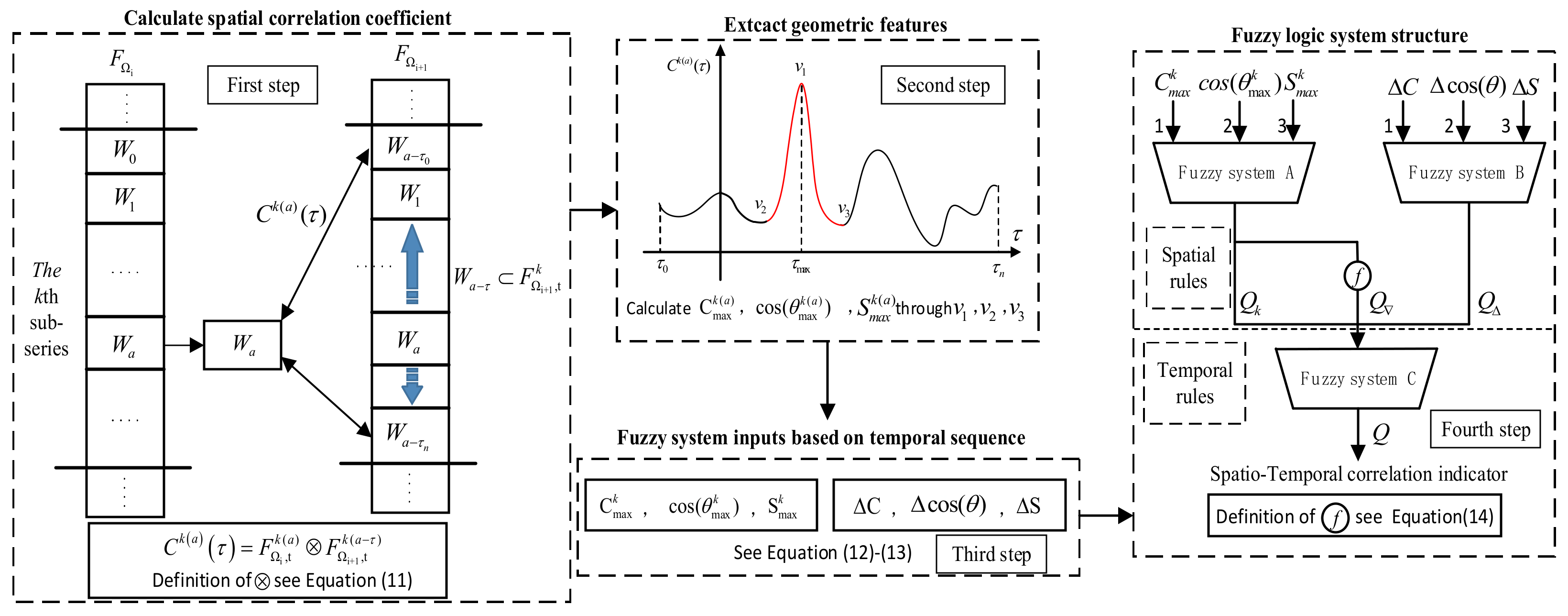
3.1. Extract System Inputs from Correlations

In order to derive the input of the fuzzy logic system from the spatiotemporal correlation, the first step, as shown in Figure 5, was to calculate the spatial cross-correlation coefficient of the abnormal node and its neighboring nodes.

$$C^{k\left(a\right)}\left(\tau \right)=F_{{\mathsf{\Omega }}_{\mathrm{i}},\mathrm{t}}^{k(a)}\otimes F_{{\mathsf{\Omega }}_{\mathrm{i}+1},\mathrm{t}}^{k(a-\tau )}$$

(11)

The node Ω_i+1 adjacent to the LTU node Ω_i, where the data changed abnormally, was identified. According to the characteristics of the dataset, the two timeseries were equally divided into several subsequences. Let $F_{{\mathsf{\Omega }}_{\mathrm{i}},\mathrm{t}}^k$ represent the k-th sub-series of $F_{{\mathsf{\Omega }}_{\mathrm{i}},\mathrm{t}}^{}$. Then, the spatial cross-correlation coefficient C^k(a)(τ) was calculated according to each sliding window W_a−τ of the given window W_a and $F_{{\mathsf{\Omega }}_{\mathrm{i}+1},\mathrm{t}}^k$ in $F_{{\mathsf{\Omega }}_{\mathrm{i}},\mathrm{t}}^k$, as shown in Equation (11). Next, a sliding time window W_a was designed with window size T and window start moment a, where W_a is the sliding time window whose window size is L and whose starting time is a, and τ introduces the delay of any integer size between windows W_a and W_a−τ of W_a−τ ∈ $F_{{\mathsf{\Omega }}_{\mathrm{i}+1},\mathrm{t}}^k$.

$$r_{X,Y}=X\otimes Y=\frac{{\displaystyle {\sum }_{i=1}^n\left(x_i-\overline{x}\right)\left(y_i-\overline{y}\right)}}{\sqrt{{\displaystyle {\sum }_{i=1}^n{\left(x_i-\overline{x}\right)}^2}}\sqrt{{{\displaystyle {\sum }_{i=1}^n\left(y_i-\overline{y}\right)}}^2}}.$$

(12)

For any two vectors X = {x₁, x₂, …, x_n} and Y = {y₁, y₂, …, y_n}, the cross-correlation coefficient between them was defined as shown in Equation (12), where $\overline{x}=\frac{1}{n}{\displaystyle {\sum }_{i=1}^n{x}_i}$, and $\overline{y}=\frac{1}{n}{\displaystyle {\sum }_{i=1}^n{y}_i}$.

According to the above calculation principle of the spatial cross-correlation coefficient, it was considered asymmetric in this paper. For example, when the LTU node Ω_i+1 was also the closest node in space to the Ω_i node, the spatial cross-correlation coefficient between nodes Ω_i and Ω_i+1 was completely different from the calculation result of the spatial cross-correlation coefficient between nodes Ω_i+1 and Ω_i. Therefore, for a certain LTU node, whether its selected neighbor node was or was not an abnormal node did not affect the obtained level of the spatial cross-correlation coefficient of the LTU node.

In the second step, the change law of the spatial correlation coefficient C^k(a)(τ) of time window W_a with respect to W_a−τ following the time delay τ was roughly as shown in the graph in the second step. In the curve, v₁ represents the peak point where C^k(a)(τ) achieves the maximum value, while v₂ and v₃ represent the two valley points below v₁. A triangle was formed by these three vertices, from which three geometric features were extracted: ${\mathrm{C}}_{\max }^{k(a)}$ is the peak point value corresponding to C^k(a)(τ) at time delay τ_max, $\cos ({\theta }_{\max }^{k(a)})$ of v₁v₂ and v₂v₃ constitute the cosine value of the included angle reflecting the rate of change from the peak point to the valley point, and ${\mathrm{S}}_{\max }^{k(a)}$ is the area of the triangle.

The third step in Figure 5 was the process of calculating the input of the fuzzy logic system through timeseries using the above features.

We can see from the time dimension that ${\mathrm{C}}_{\max }^{k(a)}$, $\cos ({\theta }_{\max }^{k(a)})$, and ${\mathrm{S}}_{\max }^{k(a)}$ represent the current temporal segment within the spatial cross-correlation of LTU nodes in order to conduct a comprehensive analysis of the spatial cross-correlation properties within the segments of historical events as the input of the fuzzy logic system. Furthermore, the history of $F_{{\mathsf{\Omega }}_{\mathrm{i}},\mathrm{t}}^k$ and $F_{{\mathsf{\Omega }}_{\mathrm{i}+1},\mathrm{t}}^k$ subseries could be used to calculate the parameters and the historical difference of characteristic parameters. There were n historical subseries, and the calculation formula is as shown in Equation (13).

$$\begin{array}{l}{\mathrm{C}}_{\max }^{k_{\mathrm{pre}}}=1/n{\displaystyle {\sum }_{i=1}^n{\mathrm{C}}_{\max }^{k_{\mathrm{pre}\_i}}}\\ \cos {(\theta )}_{\max }^{k_{\mathrm{pre}}}=1/n{\displaystyle {\sum }_{i=1}^n\cos ({\theta }_{\max }^{k_{\mathrm{pre}\_i}}}).\\ {\mathrm{S}}_{\max }^{k_{\mathrm{pre}}}=1/n{\displaystyle {\sum }_{i=1}^n{\mathrm{S}}_{\max }^{k_{\mathrm{pre}\_i}}}\end{array}$$

(13)

$$\begin{array}{l}\Delta \mathrm{C}=\left|{\mathrm{C}}_{\max }^k-{\mathrm{C}}_{\max }^{k_{\mathrm{pre}}}\right|\\ \Delta \cos (\theta )=\left|\cos {(\theta )}_{\max }^k-\cos {(\theta )}_{\max }^{k_{\mathrm{pre}}}\right|.\\ \Delta \mathrm{S}=\left|{\mathrm{S}}_{\max }^k-{\mathrm{S}}_{\max }^{k_{\mathrm{pre}}}\right|\end{array}$$

(14)

In the third step, we used the characteristic parameters ${\mathrm{C}}_{\max }^k$, $\cos ({\theta }_{\max }^k)$, and ${\mathrm{S}}_{\max }^k$ to determine the difference between the current temporal segment and the historical temporal segment as the input of the fourth step of the fuzzy logic system, as shown in Equation (14).

3.2. Design Fuzzy Logic System Structure

A set of spatial correlation characteristics of LTU nodes proposed by the comprehensive analysis could be used as a basis for measuring the level of spatial correlation. However, since the evaluation of the spatial correlation of nodes could not be obtained through a certain quantitative calculation equation, fuzzy logic could process imprecise information on the basis of the fuzzy set theory, express facts through non-numeric linguistic variables, and, finally, output numerical results. Therefore, this paper designed a cascaded fuzzy logic system. The fuzzy logic system adopts the Mamdani fuzzy inference system, which consists of two cascaded fuzzy logic systems. The fuzzy state of the input/output is defined as strong, moderate, or weak. The membership functions selected in this paper consisted of triangle type and Gaussian type membership functions, as shown in Figure 6. The mean and variance of the Gaussian membership function were 0.5 and 0.2, respectively. For the fuzzy calculation and defuzzification method of the fuzzy set, the cross-operator calculation and the area center of the gravity method were used to solve the fuzzy processing.

In the first layer of the fuzzy logic system, the Q_k of system A evaluated the spatial correlation of the current temporal segment, and the Q_Δ of output of system B evaluated the difference in spatial correlation between the historical temporal sequence segment and the current temporal segment. Both systems used spatial correlation fuzzy rules, as shown in

Table 1. Spatial correlation rules of fuzzy systems A and B.

Serial Number	Input 1	Input 2	Input 3	Output
1	Strong	Weak	Strong	Strong
2	Strong	Moderate	Weak	Strong
3	Strong	Weak	Moderate	Strong
4	Moderate	Weak	Weak	Weak
5	Strong	Weak	Weak	Weak
6	Moderate	Strong	Strong	Strong
7	Weak	Strong	Strong	Strong
8	Strong	Strong	Strong	Strong
9	Moderate	Moderate	Moderate	Moderate
10	Weak	Weak	Weak	Weak

.

$$Q_{▽}=f\left(Q_k\right)=\frac{1}{1+e^{\left|Q_k\right|}},$$

(15)

where Q_▽ is the intermediate index of the LTU space intercorrelation that represents the change rate of Q_k, as shown in Equation (15); Q_k and Q_Δ are spatial correlation indicators.

Fuzzy logic system C used temporal correlation fuzzy rules, as shown in

Table 2. Temporal correlation rules of fuzzy system C.

Serial Number	Input 1	Input 2	Input 3	Output
1	Weak	Weak	Weak	Weak
2	Weak	Moderate	Weak	Weak
3	Weak	Strong	Weak	Weak
4	Moderate	Weak	Weak	Moderate
5	Moderate	Moderate	Weak	Moderate
6	Moderate	Strong	Weak	Weak
7	Moderate	Weak	Moderate	Moderate
8	Moderate	Strong	Moderate	Weak
9	Moderate	Moderate	Moderate	Moderate
10	Moderate	Weak	Strong	Moderate
11	Moderate	Moderate	Strong	Weak
12	Moderate	Strong	Strong	Weak
13	Strong	Weak	Weak	Strong
14	Strong	Moderate	Weak	Strong
15	Strong	Strong	Weak	Moderate
16	Strong	Weak	Moderate	Strong
17	Strong	Moderate	Moderate	Strong
18	Strong	Strong	Moderate	Moderate
19	Strong	Weak	Strong	Moderate
20	Strong	Moderate	Strong	Moderate
21	Strong	Strong	Strong	Weak

, whose output Q ∈ [0, 1] was used to judge the final spatial correlation index of fault nodes and event nodes. After the final indicator Q was obtained, the self-defined threshold was set to identify the source of the anomaly. If the duration of the spatial correlation indicator continuously below the threshold exceeded two sliding windows, the LTU anomaly was judged.

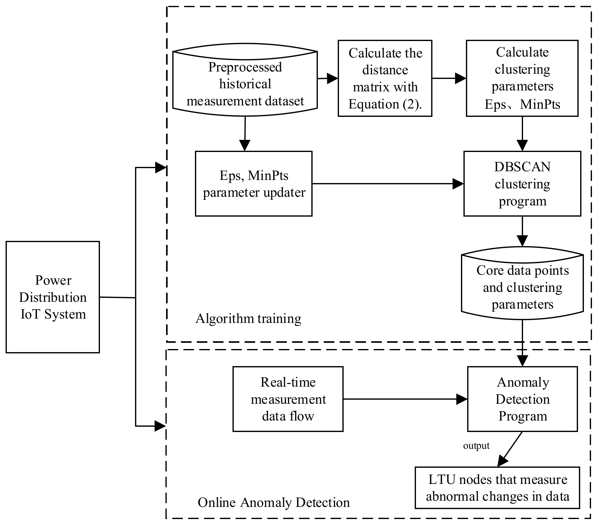
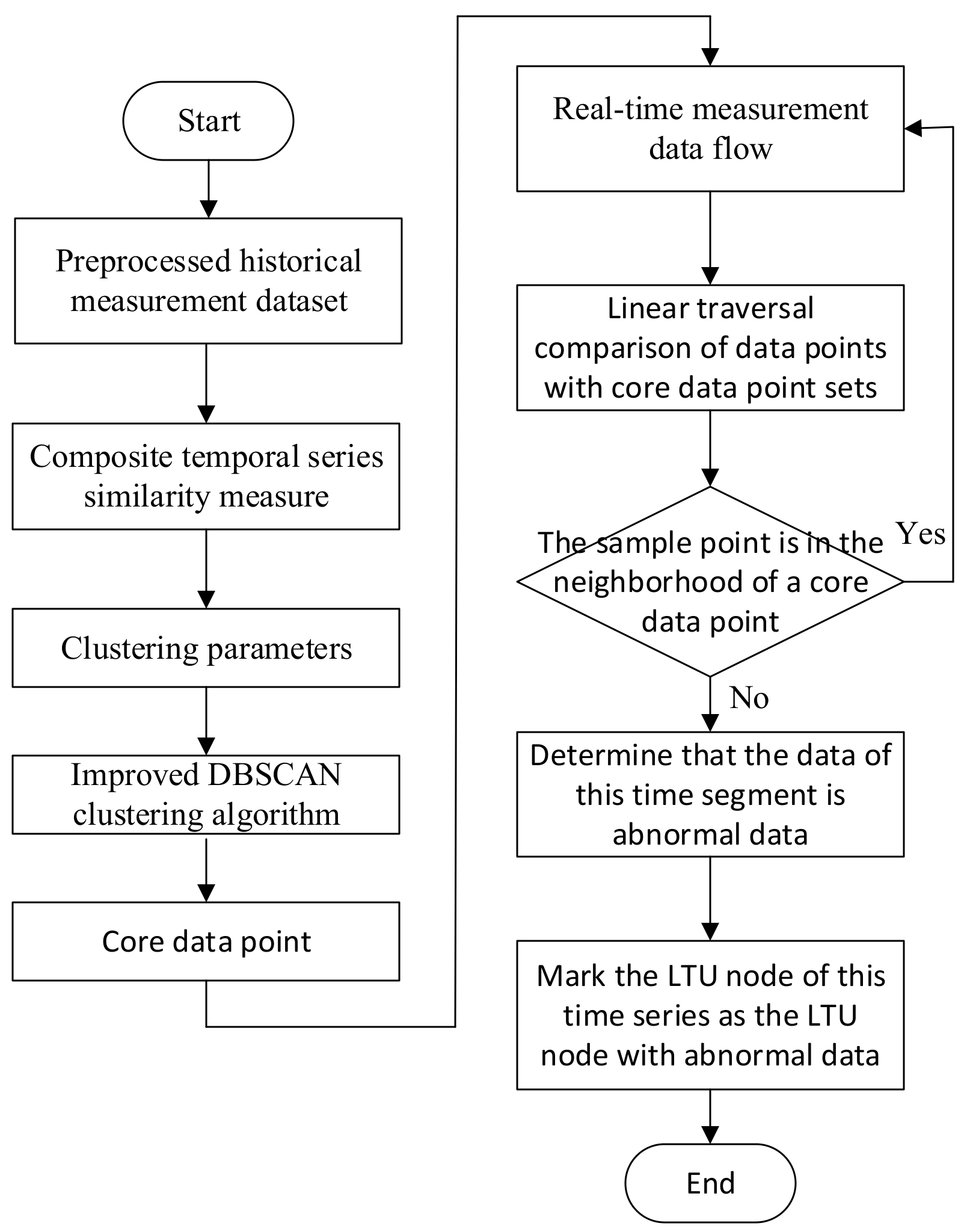
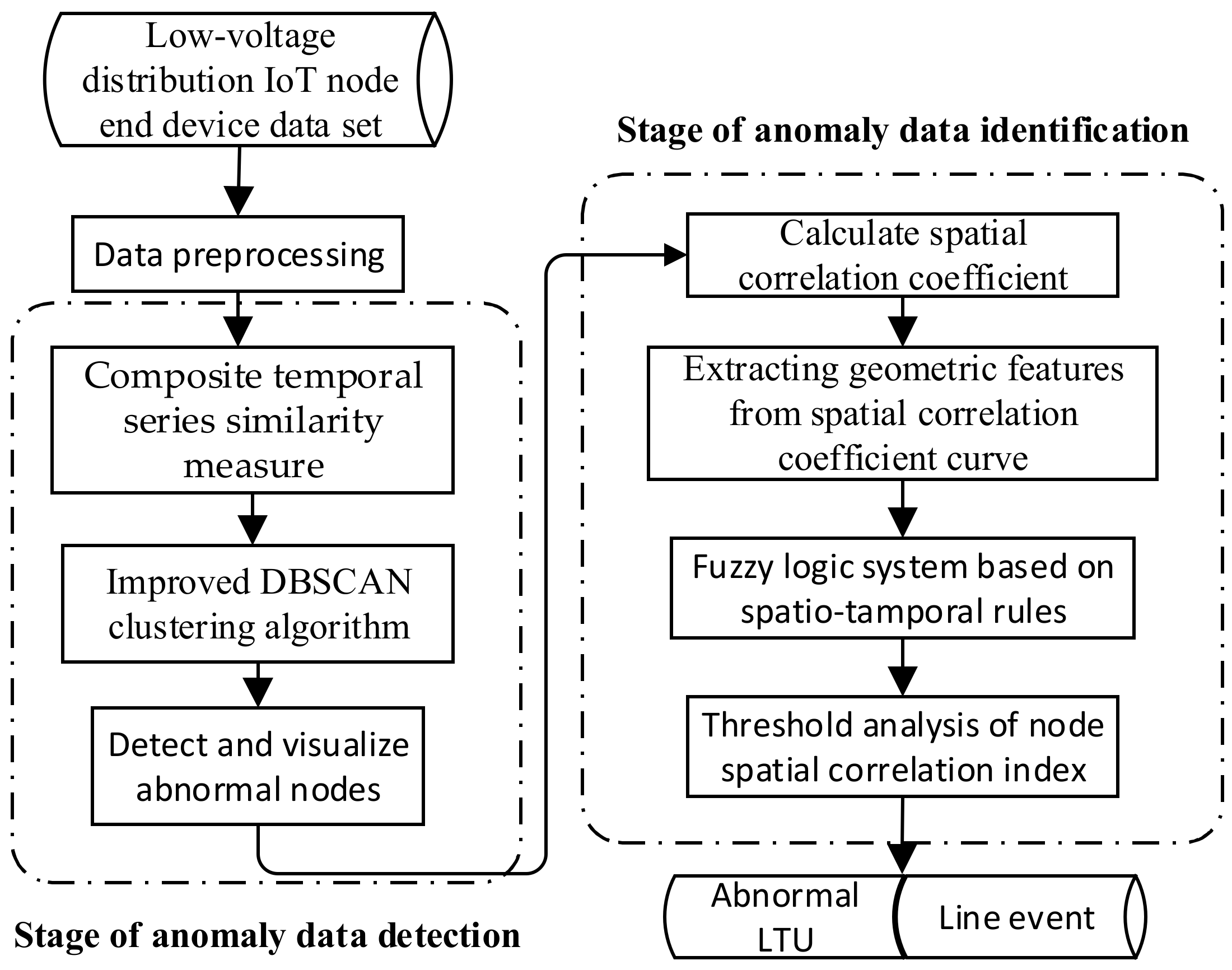
4. Overall Structure of the Algorithm

According to the extraction method of geometric features of the spatial correlation number in the above two sections, the overall structure of the algorithm for the anomaly detection and anomaly source analysis of the measured data is shown in Figure 7, which could be divided into four stages.

(I)

For the measured data of a single LTU, the distance matrix was calculated according to the composite temporal series similarity measured in Section 2.2.1. Then, the above distance matrix was used as the input for clustering the data of LTU nodes, and the noise points detected in the clustering results were the data with abnormal changes.

(II)

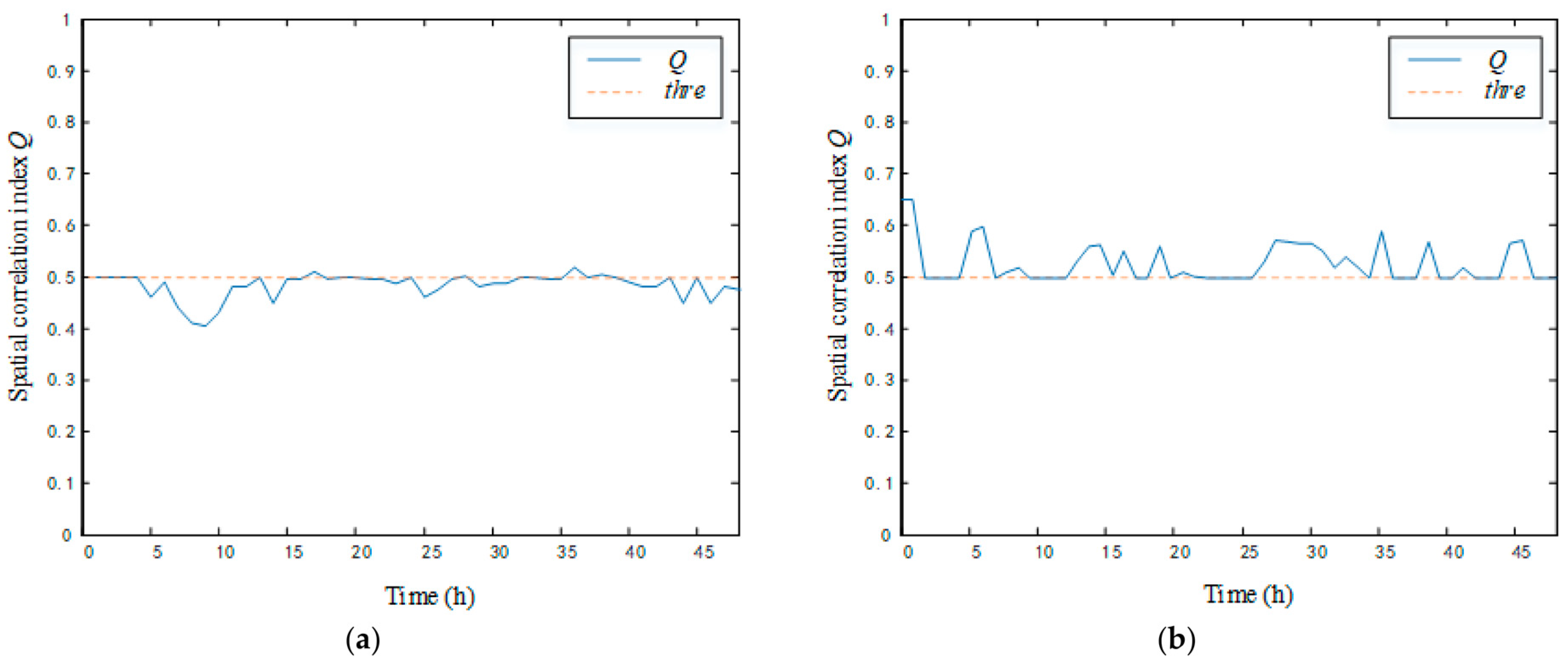
For the LTU with abnormal data changes detected, the LTU with the closest physical distance was searched, and the spatial correlation curves between the two LTUs were calculated through the sliding time window, from which the geometric features of the spatial correlation numbers were extracted.

(III)

The geometric features of spatial correlation numbers were input into the fuzzy logic system to obtain the spatial correlation index Q of LTU nodes, and the relationship between Q and the threshold thre was judged.

(1IV)

According to the data of abnormal changes in (III), the source of abnormal changes was analyzed according to the following logic:

①

If the time length of the spatial correlation index Q lower than the threshold thre was continuously greater than or equal to two sliding windows, then it was determined that the abnormal data came from the LTU failure.

②

If Q was continuously lower than the threshold thre for less than two sliding windows, the LTU was judged to work normally, and it was determined that the abnormal change data came from the line event within the LTU monitoring range.

5. Experimental Results

The LTU dataset of a power distribution Internet of Things system built by the Shandong University of Technology was used for simulation verification. The system adopts the deployment mode of a public cloud to monitor 791 LTUs in all 15 stations of the university. Part of the data were selected as the experimental dataset in this paper, including the real measured data of 600 LTU nodes for 44 days in May and June. The sampling period was 15 min/group.

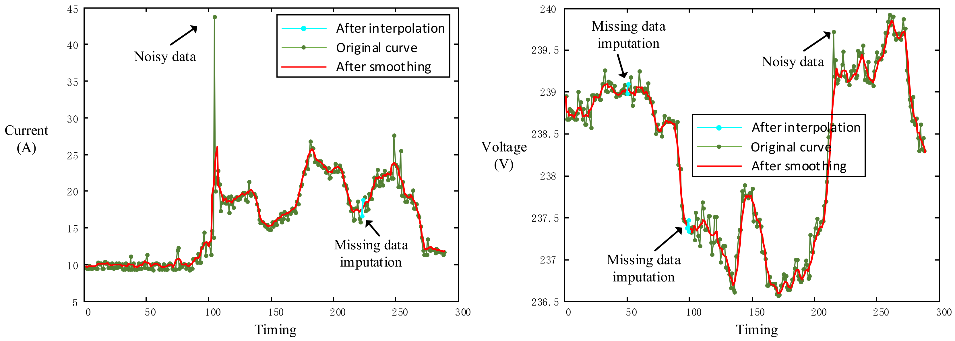
5.1. Data Preprocessing

First, the Z-score normalization method was used to normalize the data, and the measurement data of different magnitudes were converted into a unified Z-Score score. Second, the measurement dataset was cleaned. Since the LTU is a resource-constrained device, its low cost leads to the poor accuracy of its internal time synchronization device, and there may be a problem that the LTU uploads data at different times, causing the TTU or the cloud to analyze the data of a certain time section. It is difficult to obtain the complete dataset of this time section. Therefore, to solve the problems of the misalignment of data time points and missing datasets, this paper adopted the linear interpolation method. When the voltage value was negative, it was judged by the method when setting the threshold value and repaired by the nearest neighbor interpolation method. The noise data in the dataset were smoothed by the Gaussian smoothing filtering algorithm. The interpolation and the smoothing effect of the current and voltage measurement data curves of an LTU in one day are shown in Figure 8.

5.2. Experimental Settings

Due to random measurements, the dataset would not necessarily include all types of abnormal data; therefore, in this paper, through the existing distribution LTU dataset, for the artificial simulation of an abnormal state in the Internet of Things, a dataset with anomalous LTU node labels was obtained for validation, according to the common LTU anomaly states introduced in Section 2.1. Five LTU anomaly modes were defined: (a) the constant anomaly, where the measured value of the LTU was approximately a constant that could not be changed with the actual line operation; (b) the drift anomaly, where the LTU measured value deviated from the actual value at a certain rate; the error function is shown in Equation (16), where t₀ is the immediate anomaly occurring and k is the gain factor; (c) the bias anomaly, where the LTU measured value took a step within a certain period of time; (d) the impact anomaly, which refers to a sudden increase/decrease in the measured value at a certain time before quickly returning to the original sequencing sequence; (e) the periodic anomaly, where the measured data were particularly unstable, which could be represented as a periodic oscillation superimposed on the actual data. The error function is shown in Equation (17), where a₀, a_n, and ϕ_n (n = 1, 2, 3, …) are constants.

$$e=k(t-t_0).$$

(16)

$$e=a_0+{\displaystyle {\sum }_{n=0}^{\infty }{a}_n\sin (nwt+{\varphi }_n)}.$$

(17)

Following the preprocessing of the LTU measurement dataset, the data of the first 30 days were taken as the algorithm training data. The five abnormal data types described above were injected into the data of the remaining 14 days to generate a detection dataset. The ratio of normal data to abnormal data in the detection dataset was 5:5, and LTU nodes with abnormal data caused by LTU failure accounted for 60% of the abnormal data, while LTU nodes with abnormal data caused by line events accounted for 40%.

5.3. Evaluation Standard

Abnormal data detection can be converted into a binary classification task. The classification result can be a positive class P (abnormal data) or a negative class N (normal data); the confusion matrix of the final classification result is shown in

Table 3. Confusion matrix.

	Detect Result	Positive	Negative
Deal Result
Positive		True positive (TP)	False negative (FN)
Negative		False positive (FP)	True negative (TN)

.

Due to the uneven distribution of positive and negative classes in the anomaly detection dataset, in order to accurately reflect the anomaly detection performance of each comparative model, the recall rate, precision rate, and F1-score were used as the evaluation indicators of the algorithm, as expressed in the following equations:

$$\begin{array}{l}\mathrm{Recall}=\mathrm{TP} / (\mathrm{TP}+\mathrm{FN})\\ \mathrm{FNR}=\mathrm{FN} / (\mathrm{TP}+\mathrm{FN})\\ \mathrm{Precision}=\mathrm{TP} / (\mathrm{TP}+\mathrm{FP}),\\ \mathrm{F}1\text{-}\mathrm{score}=\frac{2\times \mathrm{Recall}\times \mathrm{Precision}}{\mathrm{Recall}+\mathrm{Precision}}\end{array}$$

(18)

where the recall rate reflects the abnormal data detection model’s ability to detect abnormal data and the F1-score comprehensively reflects the recall rate and precision rate.

5.4. Results

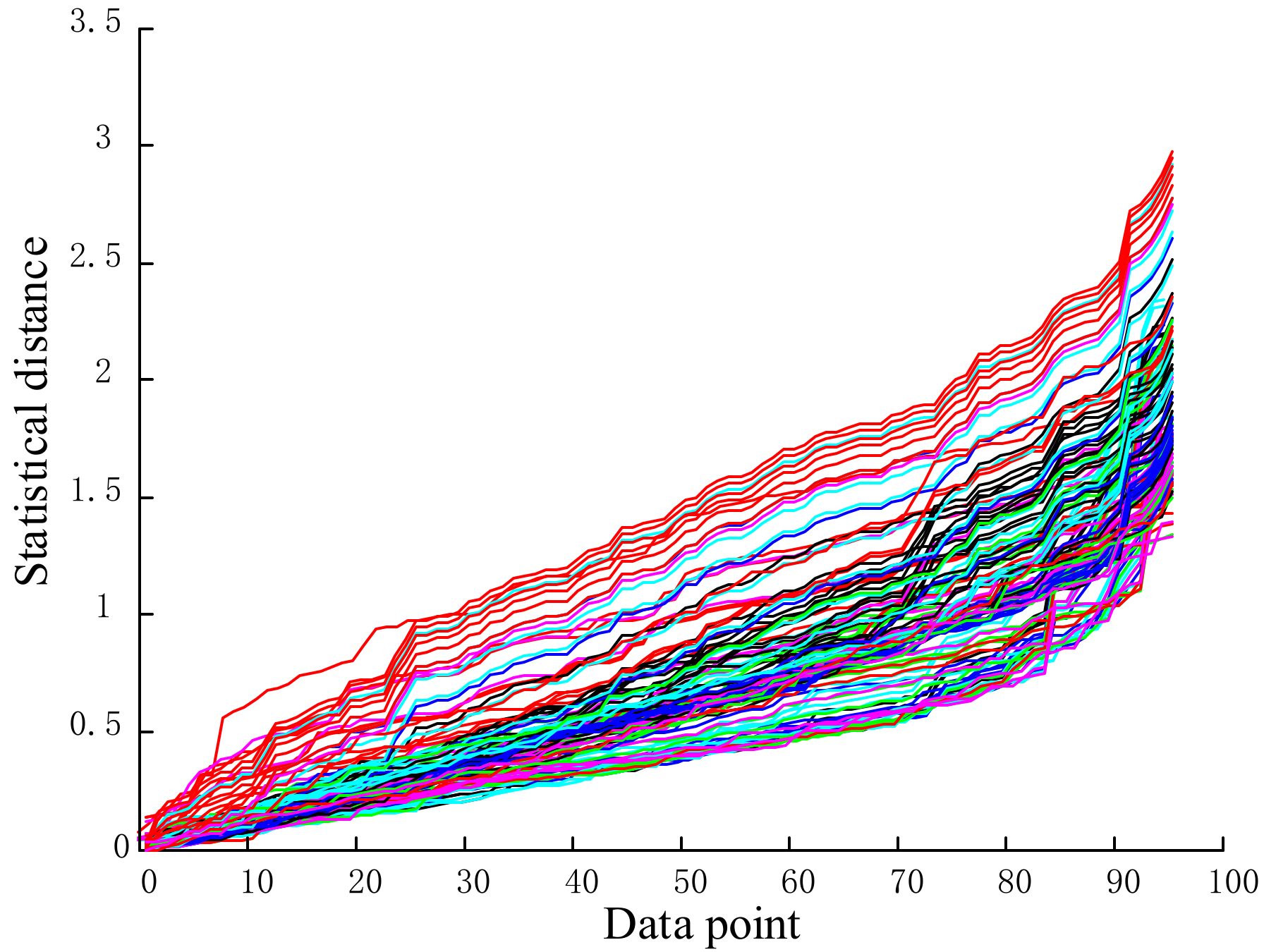
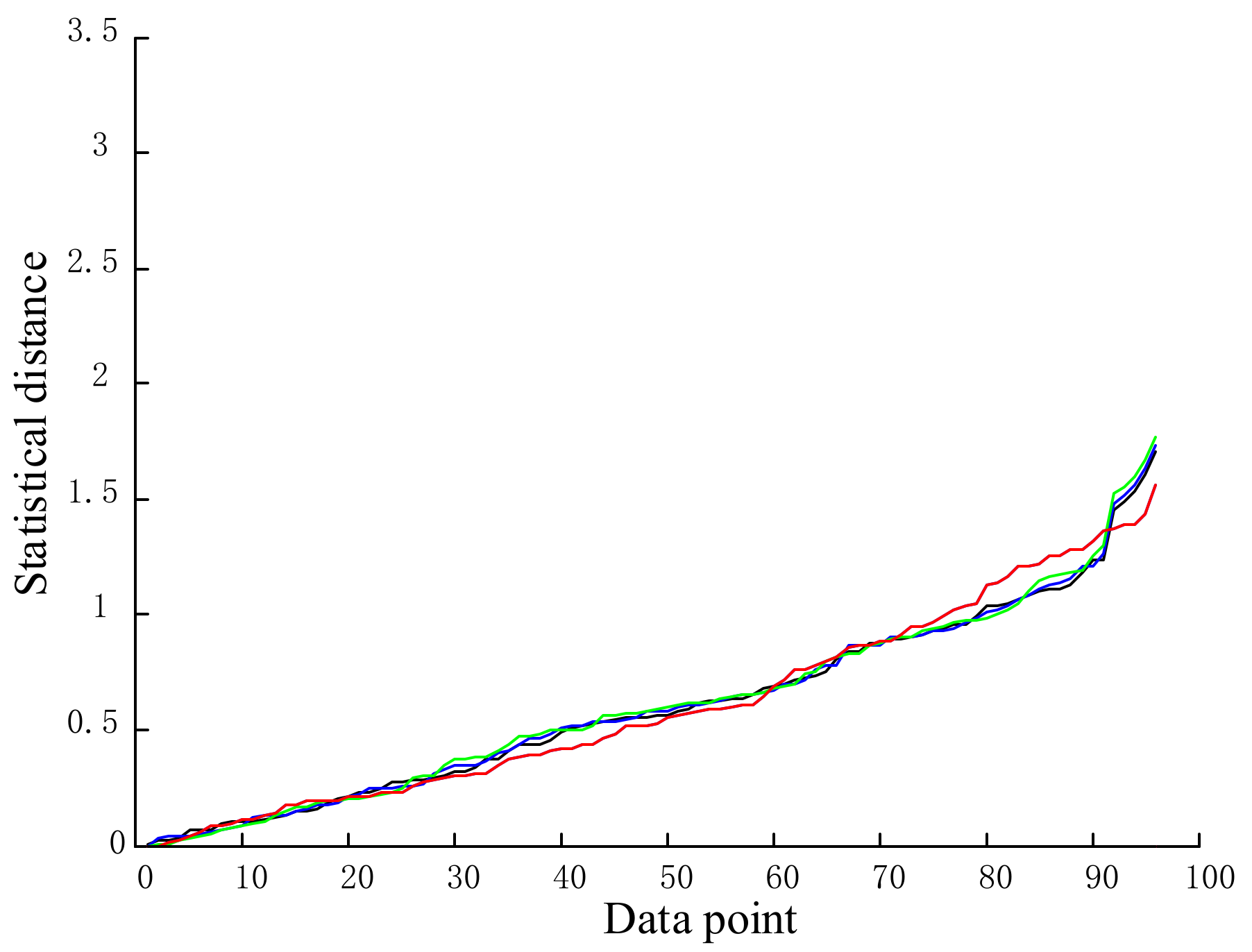
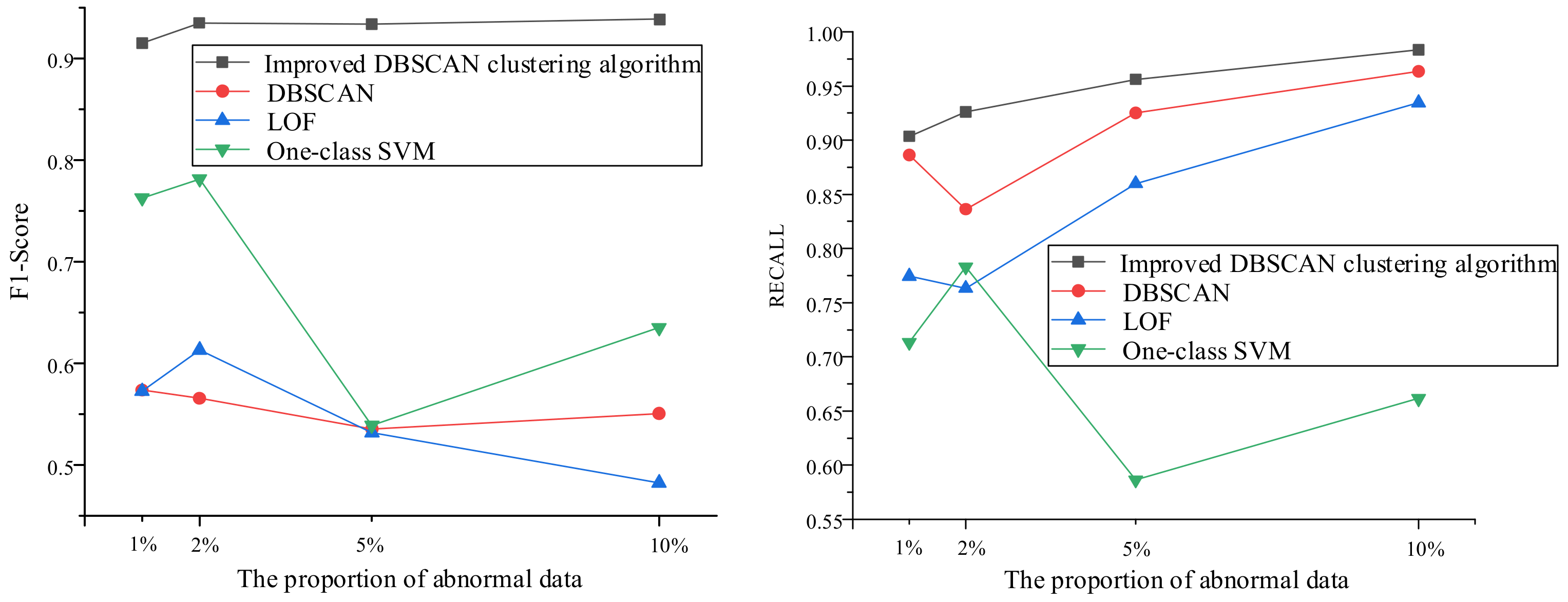
5.4.1. Anomaly Data Detection

In order to verify the effectiveness of the algorithm for abnormal data detection, the anomaly detection results of the algorithm in this paper were compared with the classic DBSCAN anomaly detection algorithm [21], LOF algorithm [22], and one-class SVM algorithm [23]. The simulation results are shown in

Table 4. Comparison of simulation results to other algorithms in the literature.

The Proportion of Abnormal Data	1%		2%		5%		10%
Algorithm	F1	Recall	F1	Recall	F1	Recall	F1	Recall
Improved DBSCAN clustering algorithm	0.9152	0.9035	0.9352	0.9260	0.9340	0.9560	0.9388	0.9833
DBSCAN	0.5737	0.8861	0.5656	0.8362	0.5354	0.9251	0.5506	0.9635
LOF	0.5726	0.7745	0.6133	0.7632	0.5319	0.8599	0.4824	0.9345
One-class SVM	0.7630	0.7131	0.7816	0.7829	0.5392	0.5863	0.6352	0.6616

and Figure 9. The abscissa of Figure 9 represents the proportion of abnormal data in the detection dataset.

As can be seen from Table 4 and Figure 9, compared with the classic DBSCAN algorithm, although the recall rate of the anomaly detection model was not much different, the F1-score of the improved DBSCAN algorithm in each anomaly proportion interval gained a significant improvement. The higher recall rate indicates a higher detection rate for abnormal data, but the lower F1-score indicates that the classic DBSCAN algorithm had a higher false positive rate. Because the improved DBSCAN algorithm effectively utilizes the temporal correlation of the LTU measurement data, in the algorithm training stage, the distance curve generated by historical measurement data could more accurately find the boundary between normal data and abnormal data, and then adaptively generate the global density parameter, such that the model could more accurately distinguish normal and abnormal data. Therefore, the F1-score was significantly improved in the datasets with different proportions of anomalies. The poor experimental performance of the LOF method was due to the uncertainty of the current and voltage measurement data distribution, which affected the k-distance of adjacent points and, thus, affected the calculation of the LOF value, resulting in a high false alarm rate of detection, which became more obvious when the proportion of anomalies was high. The low F1-score and recall of the one-class SVM algorithm were low when the proportion of anomalies was high due to the training dataset not containing all types of abnormal data, resulting in incomplete characteristics of the abnormal data learned by the detection model. Therefore, when the types and quantities of artificially simulated abnormal data increased, the types and quantities of abnormal data not learned by the model in the training set also increased, resulting in a high rate of false detections and missed detections of abnormal data by the algorithm.

It can be seen from the results that the improved DBSCAN algorithm was more stable in abnormal data detection and could detect abnormal data well for LTU current and voltage measurement data with different abnormal data proportions; the algorithm in this paper achieved a high F1-score and recall rate in abnormal data detection. A high recall rate indicates that the algorithm has a high detection rate for abnormally changed data, while a high F1-score indicates a low false detection rate. Therefore, this proves that the improved DBSCAN clustering algorithm proposed in this paper could accurately detect abnormal changes in measurement data and provide an accurate information input for the subsequent analysis of abnormal sources.

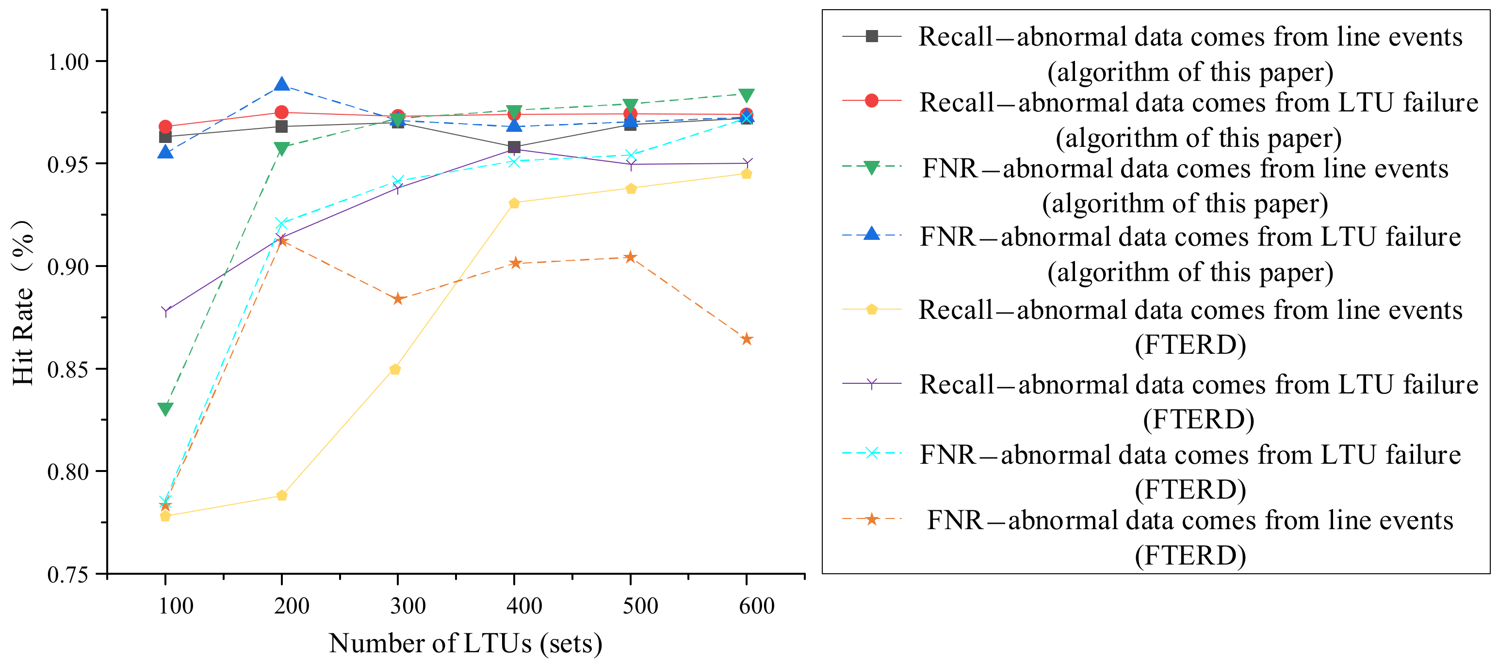
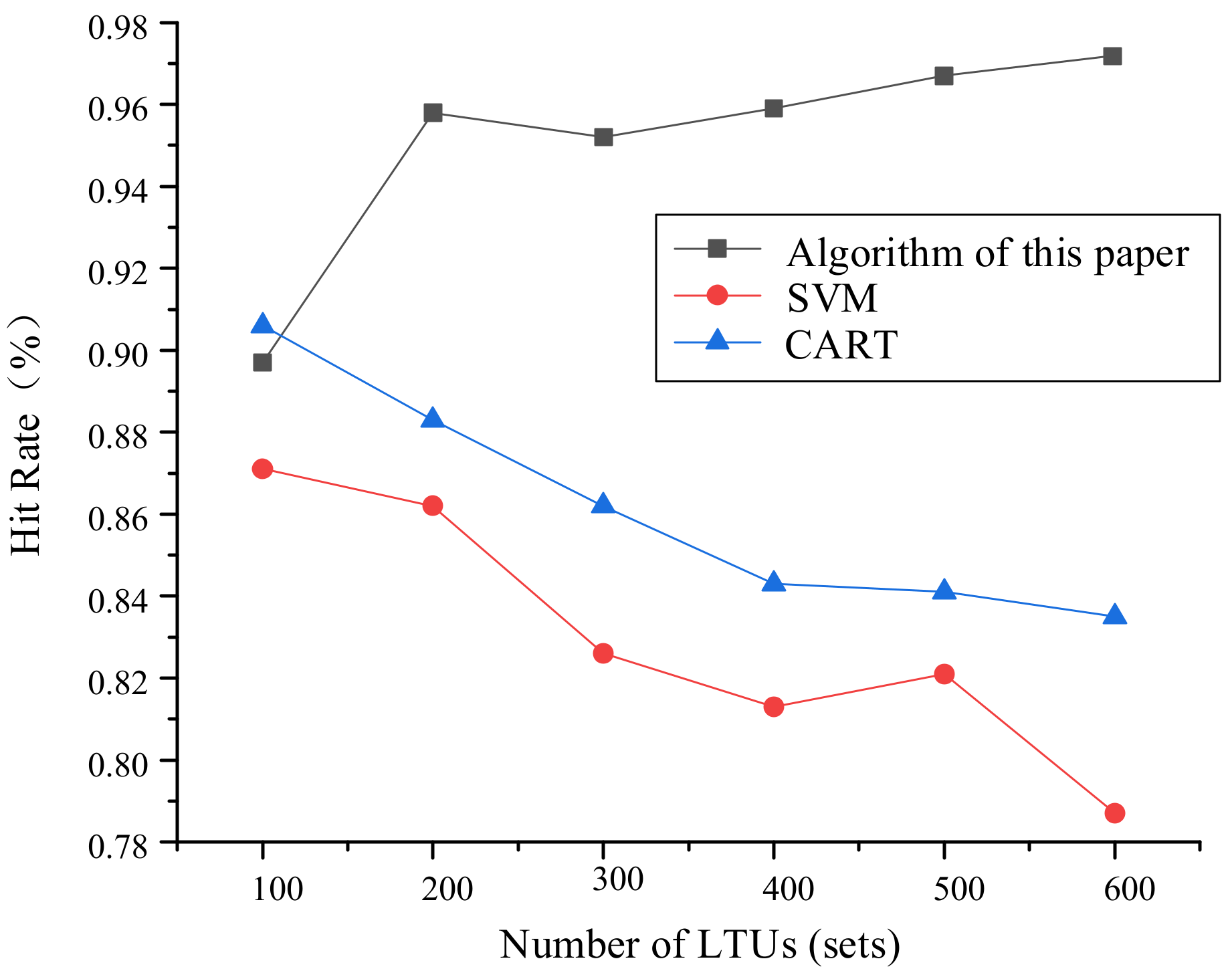
5.4.2. Source Identification of Anomaly Data

The abnormal source identification method used the spatial correlation of LTU measurement data in the distribution Internet of Things, and the spatial correlation of LTU measurement data was directly related to the LTU deployment density. Thus, in the same monitoring area, when denser LTUs were deployed, there was a smaller distance between devices and a stronger spatial correlation between measurement data. Therefore, in order to determine the detection effect of the abnormal data source identification method in the distribution Internet of Things with different density distributions, the simulation implemented measurement datasets of 100, 200, 300, 400, 500, and 600 LTU nodes from the data introduced in this chapter. The algorithm in this paper, the FTAD algorithm [24], and the classical classification algorithms SVM [25] and CART [26] were used to identify and analyze abnormal data sources according to the experimental steps described in Section 4. The simulation results are shown in Figure 10, Figure 11 and Figure 12.

The Figure 10a shows the spatial correlation index of abnormal data from LTU failures, while the Figure 10b shows the spatial correlation index of abnormal data from line events.

Figure 11 shows the simulation results of the source identification of anomaly data under different LTU scales in the distribution Internet of Things using the algorithm in this paper and the FTAD algorithm. It can be seen that the recall and precision of the FTAD algorithm were greatly affected by the scale of the LTU in the distribution Internet of Things, increasing with the increase in the number of LTUs according to the principles of the FTAD [27]. A node was confirmed to be at the event boundary if the outcome was the dominant outcome in its neighborhood, which was largely affected by the size of the LTU. The precision of the algorithm in this chapter for the detection of abnormal data caused by line events was greatly affected by the scale of LTUs. A greater number of LTUs in the distribution Internet of Things lowered the false alarm rate, because a lower LTU deployment density increased the probability of isolated LTU nodes in the feeder, while the spatial correlation between isolated LTU nodes and other LTUs was weak; thus, misjudgment could occur. However, the precision and recall of the detection of abnormal data caused by LTU failures remained above 95% under different LTU scales. Therefore, from the perspective of LTU abnormal data detection and recognition, the method in this paper is also suitable for a distribution Internet of Things with low-density LTU deployment.

Figure 12 provides a comparison of the overall accuracy of different methods under different LTU scales in the power distribution IoT, where the overall accuracy is the proportion of the total number of correctly classified samples among the total number of samples. It can be seen that the overall accuracy of the algorithm in this paper was higher than that of the other two algorithms. This was because the other two algorithms directly used the original data to train the classification model, which was not conducive to obtaining all the features of the datal; thus, the detection accuracy was low. In contrast, the algorithm in this paper extracted the spatiotemporal features of the data as the input features of the classification model, which effectively improved the detection accuracy.

6. Conclusions

In order to solve the problem that the LTU self-check and the equipment working status monitoring of the main station struggle to identify abnormal measurement data, as well as to further improve the accuracy of the LTU measurement data and ensure the accuracy and reliability of the system fault handling and advanced applications, this paper proposed an abnormal data detection and recognition method for a distribution Internet of Things monitoring terminal based on spatiotemporal correlation. Firstly, a distance matrix was calculated by the improved composite timeseries similarity measure, and the improved DBSCAN clustering algorithm was used to realize the abnormal data detection. Then, the spatial cross-correlation characteristics of LTU nodes with abnormal data were extracted using the spatiotemporal correlation of distribution IoT data, and then combined with the fuzzy logic algorithm to realize an abnormal source identification. The advantages of the method in this paper are as follows:

(1)

The algorithm proposed using the composite rule of the temporal sequence distance measurement from the probability distribution, amplitude, and error model enabled comprehensive measures in three aspects: the LTU sampling data of the timeseries similarity, the improvement of the traditional Euclidean distance similarity measure for high-dimensional data, and the improvement of the DBSCAN clustering analysis as a function of the accuracy of the information input.

(2)

Using the spatial correlation of data between adjacent LTUs in the low-voltage distribution network, the geometric characteristics of spatial correlation between abnormal data changed nodes and their adjacent nodes were extracted as the input of the fuzzy system, which successfully dealt with the complexity and relationship fuzziness of the LTU abnormal state.

(3)

The improved DBSCAN clustering algorithm based on adaptive parameter determination overcame the problem of sensitivity to the selection of global density parameters, as well as improved the flexibility and adaptability of the detection model.

(4)

Compared with traditional equipment self-inspection and equipment working state monitoring, the method in this paper could not only simplify the complex correlation of multidimensional parameters, but also identify small step anomalies, thereby enabling accurate detection.

(5)

It can be seen from the comparative simulation results that the precision and recall of the detection of abnormal data caused by LTU failures remained above 95%, while the overall accuracy remained above 90% under different LTU scales.

References

1. Liu, Q.; Zhu, Y.; Liu, G. Integrating the Power Distribution Terminals into the Power Distribution Internet of Things. In Proceedings of the 2021 Power System and Green Energy Conference (PSGEC), Online, 21–22 August 2021; pp. 62–67. [Google Scholar]
2. Lu, L.; Liu, J.; Ju, D.; Zhu, K.; Jia, Y.; Zou, D.; Chen, Y.; Qin, J.; Dai, J.; Xiang, C.; et al. Research on Security Protection Measures of the Perception Layer of Power Distribution Internet of Things. In Proceedings of the 2020 12th International Conference on Intelligent Human-Machine Systems and Cybernetics (IHMSC), Online, 22–23 August 2020; Volume 1, pp. 142–145. [Google Scholar]
3. Ma, X.; Shao, S.; Zhang, W. Research on Key Technologies of Power Distribution Internet of Things. In Proceedings of the 2020 12th IEEE PES Asia-Pacific Power and Energy Engineering Conference (APPEEC), Xiamen, China, 14–16 August 2020; pp. 1–4. [Google Scholar]
4. Fan, H.; Weng, L.; Yu, B.; Feng, X.; Chen, J.; Shou, T.; Qi, W.; Wang, D. Fault Interval Judgment of Urban Distribution Grid Based on Edge Computing of Distribution Internet of Things. In Proceedings of the 2021 Power System and Green Energy Conference (PSGEC), Shanghai, China, 20–22 August 2021; pp. 18–24. [Google Scholar]
5. Yunshuo, L.; Jian, D.; Jun, L.; Min, F.; Qing, Y. Research on distribution power quality monitoring based on distribution internet of things. In Proceedings of the 2019 14th IEEE International Conference on Electronic Measurement & Instruments (ICEMI), Nanjing, China, 1–3 November 2019; pp. 1849–1854. [Google Scholar]
6. Samparthi, V.K.; Verma, H.K. Outlier Detection of Data in Wireless Sensor Networks Using Kernel Density Estimation. Int. J. Comput. Appl. 2010, 5, 28–32. [Google Scholar] [CrossRef]
7. Sharma, K.P.; Sharma, T.P. rDFD: Reactive Distributed Fault Detection in Wireless Sensor Networks. Wirel. Netw. 2017, 23, 1145–1160. [Google Scholar] [CrossRef]
8. Zhang, K.; Shi, S.; Gao, H.; Li, J. Unsupervised outlier detection in sensor networks using aggregation tree. In International Conference on Advanced Data Mining and Applications; Springer: Berlin/Heidelberg, Germany, 2007; Volume 2007, pp. 158–169. [Google Scholar]
9. Ghorbel, O.; Ayedi, W.; Snoussi, H.; Abid, M. Fast and Efficient Outlier Detection Method in Wireless Sensor Networks. IEEE Sens. J. 2015, 15, 3403–3411. [Google Scholar] [CrossRef]
10. Karimian, S.H.; Kelarestaghi, M.; Hashemi, S. I-inclof: Improved Incremental Local Outlier Detection for Data Streams. In Proceedings of the 16th CSI International Symposium on Artificial Intelligence and Signal Processing (AISP 2012), Shiraz, Iran, 2–3 May 2012; pp. 023–028. [Google Scholar]
11. Xu, S.; Liu, H.; Duan, L.; Wu, W. An Improved LOF Outlier Detection Algorithm. In Proceedings of the 2021 IEEE International Conference on Artificial Intelligence and Computer Applications (ICAICA), Dalian, China, 28–30 June 2021; pp. 113–117. [Google Scholar]
12. Rassam, M.A.; Maarof, M.A.; Zainal, A. A Distributed Anomaly Detection Model for Wireless Sensor Networks Based on the One-class Principal Component Classifier. IJSNet 2018, 27, 200–214. [Google Scholar] [CrossRef]
13. Su, J.; Long, Y.; Qiu, X.; Li, S.; Liu, D. Anomaly Detection of Single Sensors Using OCSVM_KNN. In International Conference on Big Data Computing and Communications; Springer: Cham, Switzerland, 2015; pp. 217–230. [Google Scholar]
14. Prodanoff, Z.G.; Penkunas, A.; Kreidl, P. Anomaly Detection in RFID Networks Using Bayesian Blocks and DBSCAN. In 2020 SoutheastCon; IEEE: Piscataway, NJ, USA, 2020; pp. 1–7. [Google Scholar]
15. De Vita, F.; Bruneo, D.; Das, S.K. A Semi-Supervised Bayesian Anomaly Detection Technique for Diagnosing Faults in Industrial IoT Systems. In Proceedings of the 2021 IEEE International Conference on Smart Computing (SMARTCOMP), Irvine, CA, USA, 23–27 August 2021; pp. 31–38. [Google Scholar]
16. Ullah, I.; Mahmoud, Q.H. An Anomaly Detection Model for IoT Networks based on Flow and Flag Features using a Feed-Forward Neural Network. In Proceedings of the 2022 IEEE 19th Annual Consumer Communications & Networking Conference (CCNC), Las Vegas, NV, USA, 8–11 January 2022; pp. 363–368. [Google Scholar]
17. Aslam, S.; Herodotou, H.; Mohsin, S.M.; Javaid, N.; Ashraf, N.; Aslam, S. A Survey on Deep Learning Methods for Power Load and Renewable Energy Forecasting in Smart Microgrids. Renew. Sustain. Energy Rev. 2021, 144, 110992. [Google Scholar] [CrossRef]
18. Kiss, I.; Genge, B.; Haller, P.; Sebestyen, G. Data Clustering-based Anomaly Detection in Industrial Control Systems. In Proceedings of the 2014 IEEE 10th International Conference on Intelligent Computer Communication and Processing (ICCP), Cluj, Romania, 4–6 September 2014; pp. 275–281. [Google Scholar]
19. Wu, W.; Cheng, X.; Ding, M.; Xing, K.; Liu, F.; Deng, P. Localized Outlying and Boundary Data Detection in Sensor Networks. IEEE Trans. Knowl. Data Eng. 2007, 19, 1145–1157. [Google Scholar] [CrossRef]
20. Arena, E.; Corsini, A.; Ferulano, R.; Iuvara, D.; Miele, E.; Celsi, L.R.; Sulieman, N.; Villari, M. Anomaly Detection in Photovoltaic Production Factories via Monte Carlo Pre-Processed Principal Component Analysis. Energies 2021, 14, 3951. [Google Scholar] [CrossRef]
21. Li, X.; Zhang, P.; Zhu, G. DBSCAN Clustering Algorithms for Non-Uniform Density Data and Its Application in Urban Rail Passenger Aggregation Distribution. Energies 2019, 12, 3722. [Google Scholar] [CrossRef] [Green Version]
22. Breunig, M.M.; Kriegel, H.P.; Ng, R.T.; Sander, J. LOF: Identifying Density-based Local Outliers. In Proceedings of the 2000 ACM SIGMOD International Conference on Management of Data, Dallas, TX, USA, 16–18 May 2000; pp. 93–104. [Google Scholar]
23. Schölkopf, B.; Williamson, R.C.; Smola, A.; Shawe-Taylor, J.; Platt, J. Support Vector Method for Novelty Detection. Adv. Neural Inf. Processing Syst. 1999, 12, 582–588. [Google Scholar]
24. Peng, N.; Zhang, W.; Zhang, Y.; Huang, Z.; Zheng, L. Anomaly Detection Method for Wireless Sensor Network Based on Time Series Data. J. Sens. Technol. 2018, 31, 595–601. [Google Scholar]
25. Suthaharan, S.; Alzahrani, M.; Rajasegarar, S.; Leckie, C.; Palaniswami, M. Labelled Data Collection for Aomaly Detection in Wireless Sensor Networks. In Proceedings of the 2010 Sixth International Conference on Intelligent Sensors, Sensor Networks and Information Processing, Brisbane, Australia, 7–10 December 2010; pp. 269–274. [Google Scholar]
26. Nesa, N.; Ghosh, T.; Banerjee, I. Outlier Detection in Sensed Data Using Statistical Learning Models for IoT. In Proceedings of the 2018 IEEE Wireless Communications and Networking Conference (WCNC), Barcelona, Spain, 15–18 April 2018; pp. 1–6. [Google Scholar]
27. Florkowski, M. Anomaly Detection, Trend Evolution, and Feature Extraction in Partial Discharge Patterns. Energies 2021, 14, 3886. [Google Scholar] [CrossRef]
Figure 1. Distance curve graph.
Energies 15 02151 g001
Figure 2. Selected evaluation curves.
Energies 15 02151 g002
Figure 3. Anomaly data detection program architecture based on DBSCAN clustering.
Energies 15 02151 g003
Figure 4. Anomaly detection program flow.
Energies 15 02151 g004
Figure 5. Stepwise structure of anomaly identification stage.
Energies 15 02151 g005
Figure 6. Mixture member function adopted.
Energies 15 02151 g006
Figure 7. The overall structure of the algorithm.
Energies 15 02151 g007
Figure 8. Example diagram of current and voltage curve interpolation and smoothing processing.
Energies 15 02151 g008
Figure 9. F1-score and recall of improved DBSCAN clustering algorithm, DBSCAN algorithm, LOF algorithm, and one-class SVM algorithm under different proportions of abnormal data.
Energies 15 02151 g009
Figure 10. Spatial correlation index curve of abnormal data from LTU failures (a) and abnormal data from line events (b).
Energies 15 02151 g010
Figure 11. The detection rate of the proposed algorithm and the FTAD algorithm with LTU scales in the distribution Internet of Things.
Energies 15 02151 g011
Figure 12. The overall accuracy of different algorithms under different LTU scales in a distribution Internet of Things.
Energies 15 02151 g012