Study on Flow Characteristics and Mass Transfer Mechanism of Kettle Taylor Flow Reactor

Abstract

A scheme of a gas–liquid mixed jet is designed by installing gas distributor at the bottom of a stirred tank reactor to generate Taylor vortex. The eddy flow characteristics and mass transfer mechanism in the reactor are analyzed by numerical simulation and experiment. The results show that the evolution law of Taylor vortex in a stirred tank reactor with a rotating Reynolds number is similar to that in a conventional Taylor reactor. The Taylor vortex generated in the stirred tank reactor creates a partial plug flow region in the original complete mixing flow pattern, which reduces back mixing, the plug flow area expands with the increase of rotating Reynolds number. Under the condition of a critical rotating Reynolds number (Re_cr), the gas phase homogeneity of the reactor is increased by 28% and the dissolved oxygen rate is increased by about 5 times, which effectively improves the flow condition in the reactor and strengthens the mass transfer efficiency between the gas and liquid. The research results provide a theoretical basis for breaking through the limitation of small reaction space of conventional Taylor flow reactor and expanding production scale. The refit of kettle reactor is universal and easy to operate.

1. Introduction

The stirred tank reactor is widely used in chemical, petroleum, biological and other fields [1,2,3,4]. The stirred tank reactor is stable, reliable and flexible in continuous production, but it is not suitable for reactions with high conversion rates because of the back mixing of fluid in the reactor caused by stirring [5]. In this paper, the Taylor vortex is introduced into a stirred tank reactor to improve the flow and mass transfer characteristics of the reactor by designing a scheme of a gas–liquid mixed jet. The Taylor vortex is a fluid motion existing between two coaxial cylinder annulus; a series of axial alternating and orderly secondary vortices are generated between the annulus through the relative rotation of the inner and outer cylinders [6]. The basic structure of the conventional Taylor flow reactor is shown in Figure 1.

Since its discovery in 1923, the flow stability and formation of toroidal vortex (Taylor vortex) has attracted extensive attention from scholars inland and abroad. The early studies on Taylor flow mainly focused on the theoretical research of the flow diagram, flow stability and transmutation mechanism under different flow conditions. Four types of flow have been recorded by Kaye and Elgar [7]: laminar flow, laminar flow with Taylor vortex, turbulent flow and turbulent flow with Taylor vortex. Recent studies have proved that the axial back mixing in the Taylor flow reactor is small and the reaction driving force is high, and the existence of Taylor vortex will strengthen the heat and mass transfer of the reactor [8,9].

Recent research has focused on the application of Taylor flow in reactors and other devices. Centrifugal extractor [10], biological reactor [11], nuclear main pump [12] and other equipment based on the Taylor vortex principle have developed rapidly in the field of industrial production. In the past few years, different configurations have been used to enhance the heat and mass transfer capacity of Taylor vortex in reactors. Giordano et al. [13,14] tested the flow modes and mass transfer characteristics of the Taylor flow reactor under different operating parameters. The performance of the reactor was evaluated by a mathematical model which laid the foundation for experimental research. Resende et al. [15,16] extended the mathematical model established by Giordano to a liquid solid reaction, and studied the suspension distribution characteristic of catalyst particles in a Taylor flow reactor. They established a comprehensive calculation model for the mass transfer parameters of two phases. Ostilla-M’onico et al. [17] numerically explored the transition of the Taylor Couette flow to the ultimate flow regime with various gap widths and found that the transition is delayed in the wide gap, owing to the combined effects of the stabilizing curvature of the inner cylinder and the reduced shear. Ritcher et al. [18] and Deng et al. [19] studied how the flow state changes in the Taylor flow reactor after changing the rotor shape and adding internal baffles, focusing on improving the reactor performance through structural changes. M. Carlos Álvarez et al. [20] incorporated annular fins over the inner rotating surface and found that annular fins disturbed the Taylor–Couette flow behavior by reducing the smooth critical Taylor number (Ta = 57.18). Yang Guang et al. [21] found through simulation that the Taylor vortex column generated by the co-axial inversion of the double-blade can enhance the gas dispersion ability and improve the overall gas holdup. Pieter et al. [22] found that the generation and evolution of Taylor vortex—when the outer cylinder was fixed—was more stable than when both the inner and outer cylinders were rotating by setting different speeds. Dennis et al. [23] found that the roughness—changing along the span—can control the wavelength of the Taylor vortex by changing the roughness of the cylinder wall in the Taylor reactor.

The above research plays an important role in improving the heat and mass transfer of Taylor vortex, but there are still limitations in the practical application of the Taylor vortex: Because of the limitation that Taylor vortices can only be generated at a small annulus ratio, Taylor flow reactors in the existing literature are mostly tubular in structure, which means they are generally small in volume and the amplification effect is limited. It is difficult to meet the needs of large-scale industrial production.

In this paper, based on the stirred tank reactor, a stirred tank Taylor reactor is built; it inherits the advantages of the tubular flow reactor Taylor and overcomes its limitation in large-scale industrial application. On the basis of the Taylor flow improvement and mass transfer, the reactor not only effectively improves the reaction space and increases the output, but is also easy to refit and has strong generalization. A gas distributor system consisting of a gas collect box, three nozzles and three static distributors is installed at the bottom of the stirred tank reactor. The static distributors are evenly distributed under the agitator and connected with the gas collector box through the nozzles. Taylor vortex is formed in the stirred tank reactor. The reactor structure constructed is shown in Figure 2.

In this paper, the stirred tank Taylor reactor is compared with the conventional Taylor flow reactor; the gas–liquid two-phase flow in the reactor is numerically simulated by CFD technology and compared with the experimental results, providing guidance and reference for the study of the flow characteristics and mass transfer mechanism of the reactor.

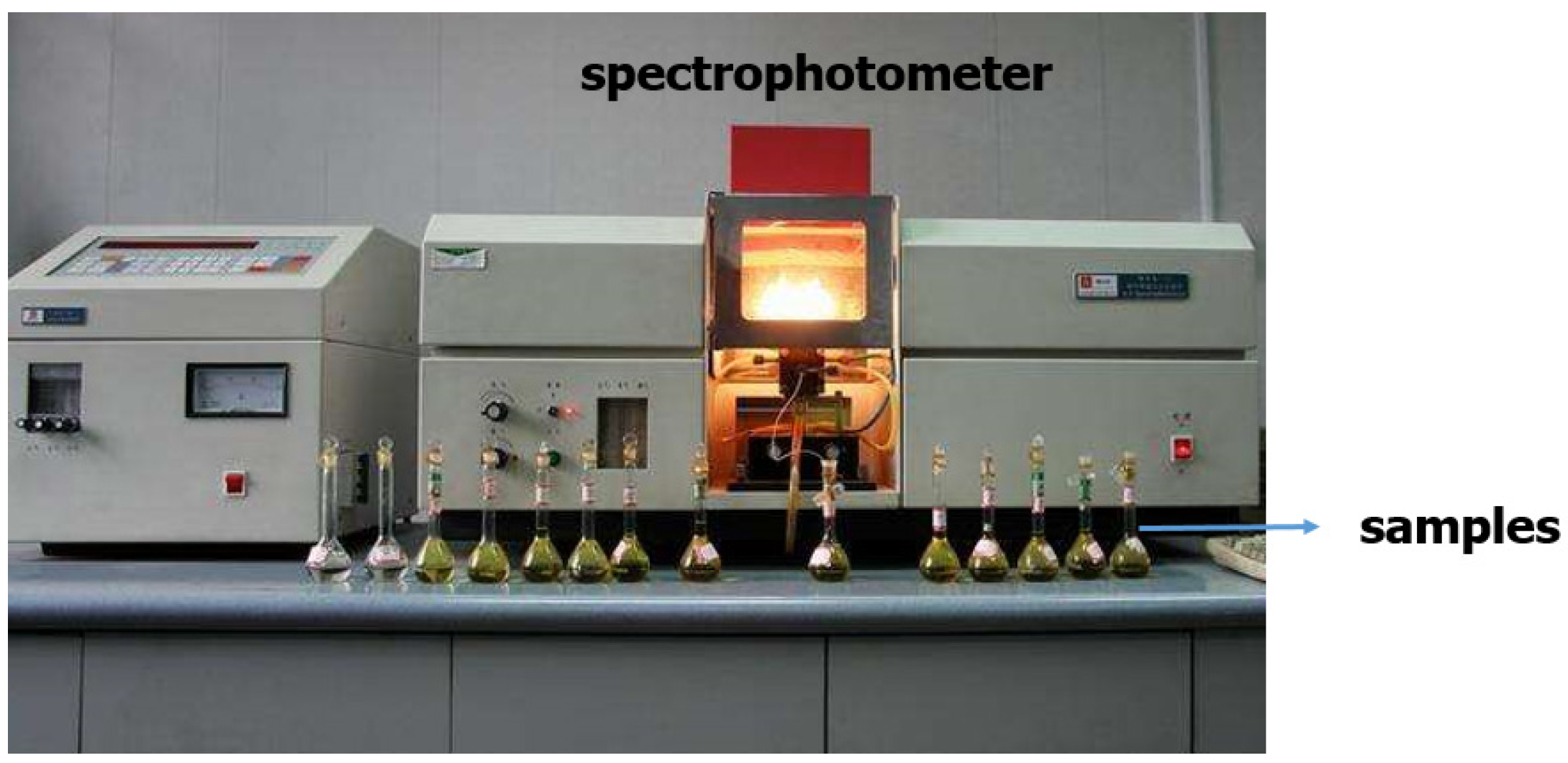
2. Experimental Equipment and Procedures

The experimental device consists of a stirring system, a kettle reactor and an air distribution system, as shown in Figure 3. The stirring system is a three-phase asynchronous motor that drives the rotating shaft through a coupling to carry out mechanical stirring. The main part of the reactor is composed of a Φ 370 × 1150 stainless steel cylinder connected with a stainless steel head; the air distribution system consists of a vent tube, a distributor box, three nozzles and three Kenneth static mixers. Air is mixed with water at the inlet of the turbulence pump, the high-speed impeller repeatedly cuts the air into small bubbles in the pump housing, it dissolves rapidly in water and forms dissolved gas water under high pressure, which then enters the reaction vessel. The static mixers are aligned with the nozzle outlet and the collect box ensures even air separation. The high-speed air suction fluid generated at the nozzle outlet enters the static mixers together with the air flow to produce mixing, which generates the Taylor vortex in the process.

A total of 100 L water is added into the reactor to start stirring and air is pumped through the vortex pump. The experimental conditions are as follows: set the stirring speed at 250 rpm, set the air input flow rate at 0.001 kg/s.

After the rotating flow reaches a stable state, a syringe is used to rapidly inject 2% potassium permanganate solution (1 mL) as a colored tracer from the inlet. Start timing when colored tracer is injected; sample every 10 s at the outlet sampling port and stop sampling at 300 s. The absorbance value of the samples is determined by colorimetric analysis using a spectrophotometer, as shown in Figure 4. The basic principle of colorimetric analysis of concentration is based on the Lambert–Beer law. The absorption effect of the material on light. Therefore, at a certain wavelength, the absorption intensity increases with the increase of the concentration of the material; that is, the concentration of the material is proportional to the degree of light absorption. The mathematical expression is shown by Formula (1):

$$\mathrm{A}=\log \frac{1}{T}=kbc$$

(1)

where A is the absorbance; T is the transmittance; k is the molar absorption coefficient; b is the thickness of the absorption layer, that is the thickness of the colorimetric cup in the spectrophotometer; c is the concentration of the light-absorbing substance.

Distilled water is used as blank control and the spectrophotometer is used to scan automatically at the wavelength of 440~580 nm. The maximum absorption peak wavelength (525 nm) is selected from the absorption spectrum curve of potassium permanganate solution and the corresponding absorbance was measured at 525 nm.

3. Numerical Simulation

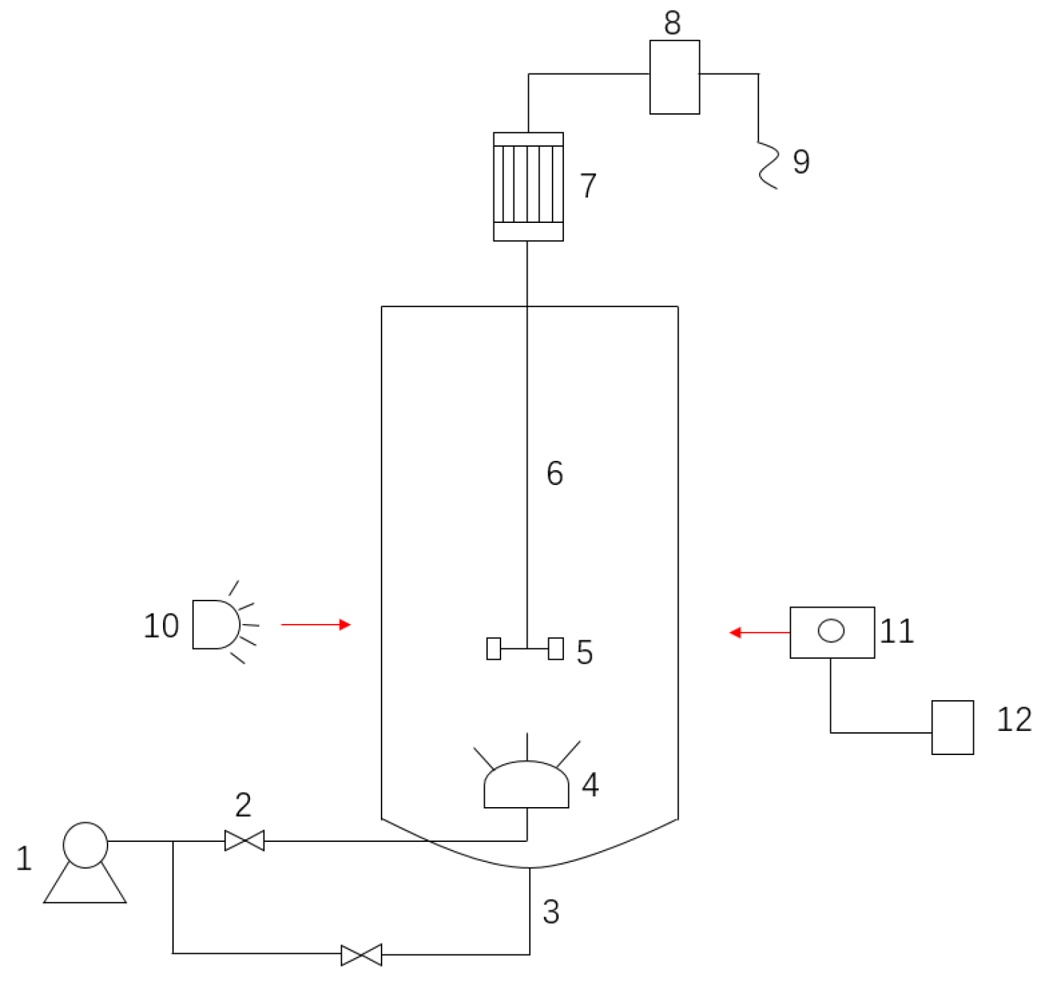
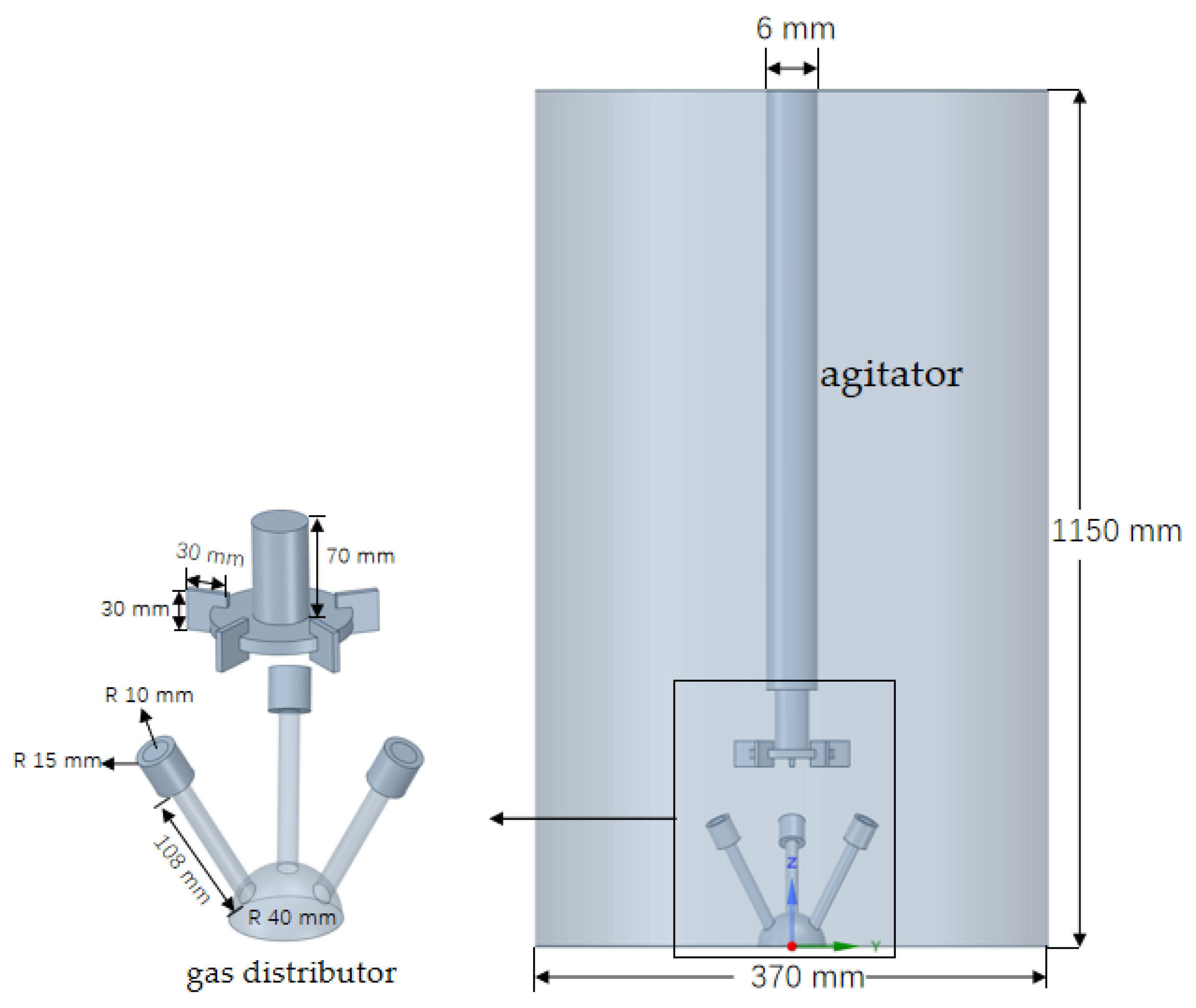
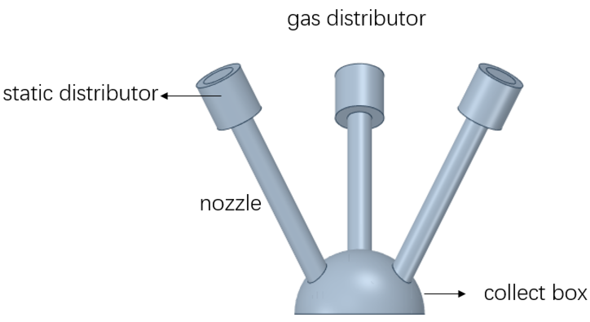
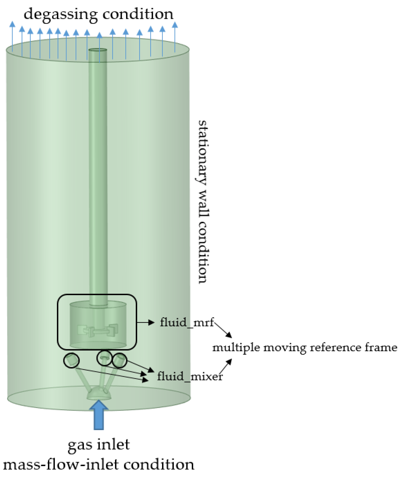
3.1. Geometric Model

Figure 5 is a schematic diagram of the stirred tank Taylor reactor geometric model. The dimensional parameters are shown in

Table 1. Reactor size parameter.

Parameter	Reactor Diameter	Reactor Height	Agitator Diameter	Static Distributor Diameter	Nozzle Length	Annulus Ratio
Dimensions (mm)	370	1150	6	30	108	7.42

. The annulus ratio is defined as the ratio of the reactor gap width to the agitator radius. The static distributor is designed as a small cylinder rotating around an axis, as shown in Figure 6. The liquid phase flows into the torus and rotates with the gas phase between the annulus of the small cylinder. The mixing process of the gas phase and liquid phase is simulated when the mixture enters the static distributor and is broken into small bubbles and jet out.

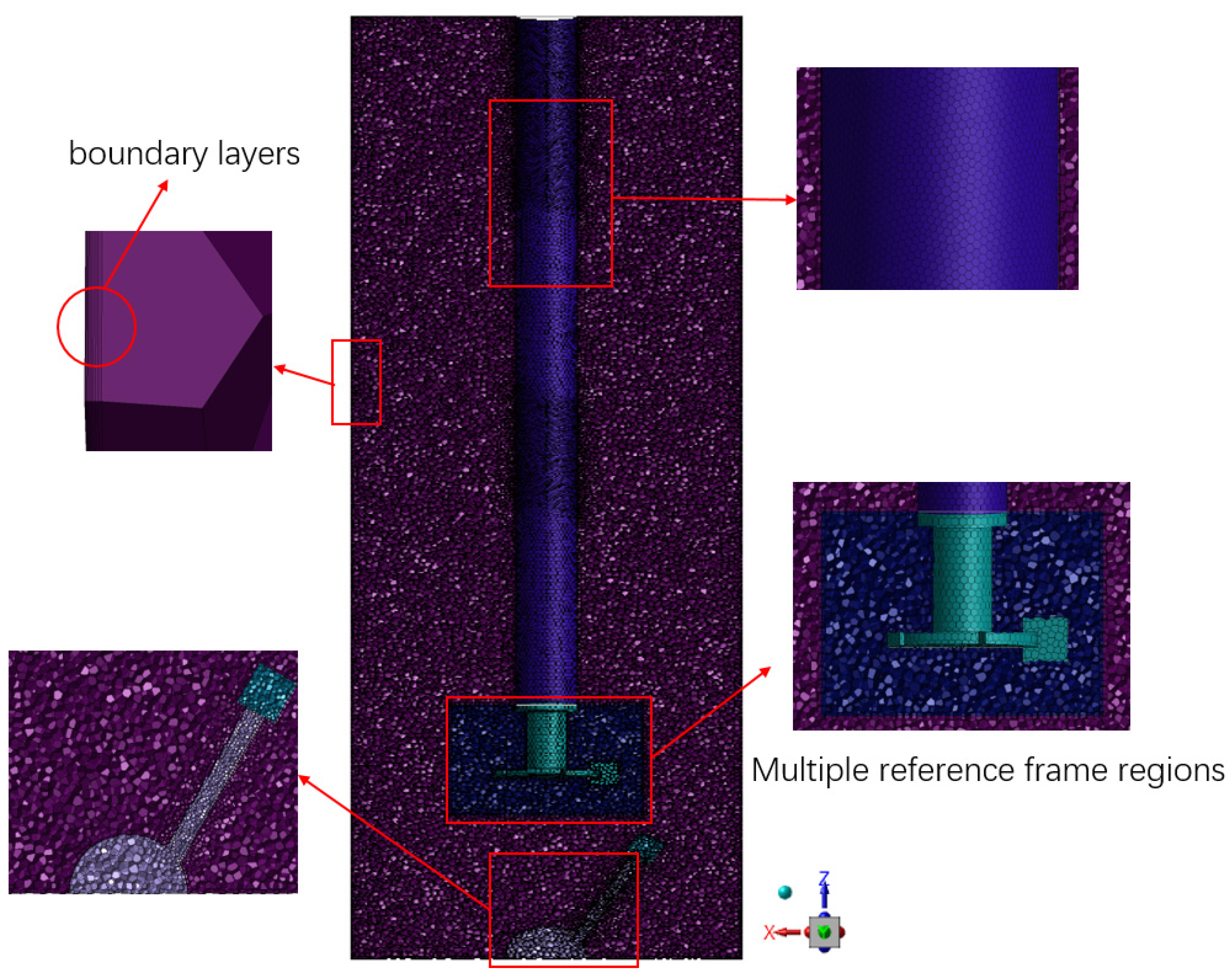
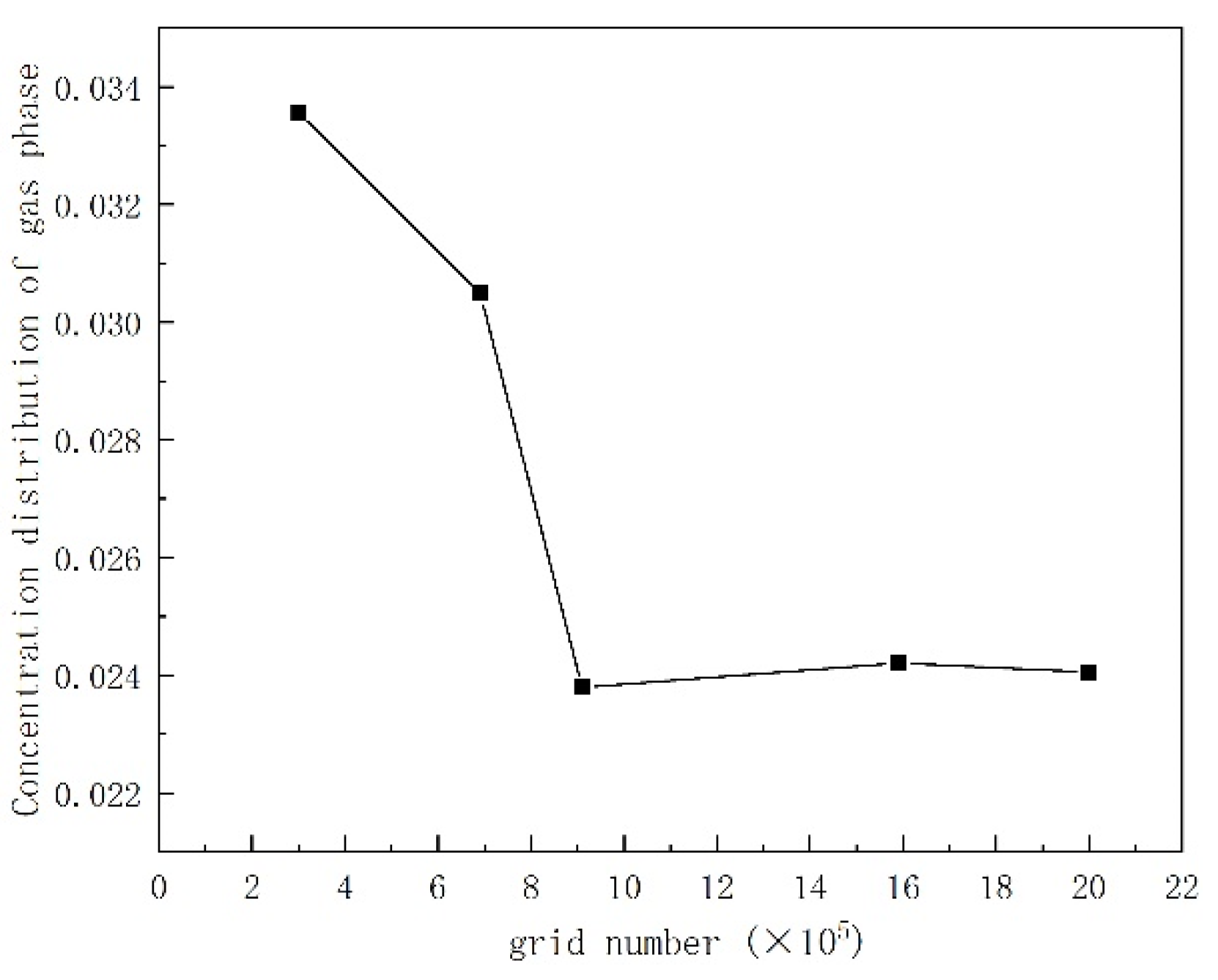
3.2. Grid Division and Grid Independence Verification

The CFD software ANSYS Fluent is used to generate mesh of the reactor, unstructured hexahedral mesh is used for mesh division in Fluent Meshing and a local mesh encryption is used for blade area and gas distributor area. Five grid sizes are selected to study the influence of different mesh numbers on numerical simulation and the boundary layer is divided into a total of 10 layers. The offset method type called uniform is used to determine how the mesh cells closest to the boundary are generated. The thickness of the first layer is 0.01 mm and the growth rate is 1.2. Figure 7 shows the schematic diagram of volume and boundary layer grids at Y = 0 section when the total number of grids is 914,523. The grid quantity and the y+ values are shown in

Table 2. Reactor grid quantity and Y + value.

Grid Quantity	Y+
301,545	34.28
693,835	37.51
914,523	32.15
1,593,471	30.16
2,664,228	31.31

.

Figure 8 shows the average gas phase concentration at the outlet of the reactor of numerical models with five grid sizes under the same working condition. It can be seen from the figure that when the quantity of grid reaches 914,523, as the quantity of grid increases, the gas phase concentration at the exit has little change and the difference of average gas phase concentration between the quantity of grids at 1,593,471 and the quantity of grids at 914,523 is 8.3% (<10%). Therefore, combined with the time consuming and accuracy of simulation, a total of 914,523 grids are selected for numerical simulation.

3.3. Physical Model and Boundary Conditions

The CFD simulation process is conducted using ANSYS Fluent 2021 software; as the research object is multiphase flow, the 3D and double precision mode is selected to open Fluent [24]. A pressure-modified algorithm is used to set the solver, the advantage of which lies in solving incompressible flow. A pressure-velocity coupling algorithm includes SIMPLE algorithm and PISO algorithm; considering the complexity of the two-phase flow field in the reactor, SIMPLE algorithm is chosen to solve the problem.

Gravity is enabled in the operating conditions to account for gravitational forces; the gravity acceleration in the Z direction is set as −9.81 m/s² and the operating pressure is retained as 101,325 Pa. When dealing with gas–liquid two-phase flow in the reactor, the Eulerian multiphase model is used, the Laminar model and standard k-ε turbulence model with standard wall functions is enabled and the dispersed turbulence model is selected according to different working conditions. The continuity equation and momentum equation were formulated as follows:

$$\frac{\partial {\rho }_k}{\partial \mathrm{t}}+{\nabla }_g({\rho }_k{u}_k)=0$$

(2)

$$\frac{\partial {\rho }_k{u}_k}{\partial \mathrm{t}}+{\nabla }_g({\rho }_k{u}_k{u}_k)=-{\nabla }_g{P}_{k}I+{\nabla }_g{T}_k+{\rho }_k{g}_k$$

(3)

where subscript k represents phase (k = g represents gas phase, k = l represents liquid phase); ${\rho }_k$ is the density; $u_k$ is the velocity vector; $P_k$ is the pressure scalar; $I$ is shear stress tensor; and $g_k$ is the acceleration vector of gravity.

Water and air are added to the list of fluid materials and liquid water is specified as the primary phase while air is specified as the secondary phase, the diameter of the air bubbles is set to 1.5 mm [25]. The grace model is selected as the interphase interactions formulation, which is suitable for liquid-gas mixtures with low gas density and bubble sizes of 1–2 mm and the Surface Tension Coefficients is set as 0.073 N/m. In the dialog of mass transfer mechanisms, the diffusion coefficient of oxygen in liquid water is set as 2.1 × 10⁻⁹ m²/s, the principle of material transfer between the gas and liquid phase adopts the double film theory: Oxygen in the air is transferred to water through the phase interface and the mass transport equation of oxygen components in the gas-liquid two phases is expressed as follows:

$$\frac{\partial }{\partial t}({\alpha }_k{\rho }_k{Y}_{o,k})+\nabla ({\alpha }_k{\rho }_k{u}_k{Y}_{o,k})=\nabla \left[{\alpha }_k{\rho }_k{D}_{o,k}\frac{{\mu }_{eff,k}}{{\mu }_k}(\nabla Y_{o,k})\right]-k_{l}a{\alpha }_k{\rho }_l(Y_{o,l}^{*}-Y_{o,l})-S_0$$

(4)

where ${\alpha }_k$, ${\rho }_k$, $u_k$, ${\mu }_{eff,k}$, ${\mu }_k$ are phase holdup, density, velocity, effective viscosity and viscosity respectively; $Y_{o,k}$ is oxygen mass fraction; $Y_{o,l}^{*}$ is the mass fraction of liquid phase saturation of oxygen relative to gas phase partial pressure; D_o,k is the diffusion coefficient of oxygen; a is specific surface area between gas and liquid phase; $S_0$ is the source term of oxygen consumption, in the gas phase, S₀ = 0.

The mesh has five fluid cell zones: fluid_mrf is a zone associated with the stirring blade, fluid_mixer1, fluid_mixer2 and fluid_mixer3 are zones associated with three static distributors respectively and fluid_reactor represents the rest of the reactor. These zones ars divided using multiple reference frame method to model the flow around rotating parts as steady-state with respect to the moving frames [26]. Frame Motion is selected to set up the cell zone conditions for the fluid zone associated with the rotating parts. The rotation-axis direction of the fluid zone associated with the stirring blade (fluid_mrf) is set to the value of (0, 0, 1) for X, Y and Z and the speed of rotational velocity is set according to different rotational Reynolds number. The rotation-axis direction of the fluid zones associated with the three static distributors (fluid_mixer1, fluid_mixer2 and fluid_mixer3) is set as the axis of the respective static distributor and the speed of rotational velocity is set to 200 rpm.

Coupled scheme and Pseudo-Transient are selected under Pressure Velocity Coupling in the Solution Methods. Pseudo transient explicit relaxation factors of pressure and momentum are set to 0.2 and 0.3, respectively.

The conditions on the boundaries of the domain are defined as follow: Since each wall uses the same reference frame as the cell zone within which they are located, all walls will use the default stationary wall condition. The top of the reactor uses the degassing boundary condition, which only allows gas phase to leave the domain. Set mass-flow-inlet condition at the gas inlet for the secondary phase (air), set mass flow rate at 0.00102 kg/s and set 1 for volume fraction. The figures of the domain is shown in Figure 9.

Parameter settings are shown in

Table 3. Parameter setting.

Inlet Mass Flow Velocity	Static Distributor Speed	Stirring Speed	Rotating Re Number
0.001 kg/s	200 rpm	50 rpm	19,000
		150 rpm	57,000
		250 rpm	95,000
		350 rpm	133,000

. Four different working conditions are selected to analyze the flow field evolution law in the reactor by change the value of the rotating Reynolds number. The rotating Reynolds number is defined as:

$$\mathrm{Re}=\frac{d_j^{2}n\rho }{\mu }$$

(5)

where d_j is the diameter of agitator; n is stirring speed; ρ is the material density; μ is viscosity of material.

When the continuity residual curve and concentration residual curve decrease to below 10⁻⁴ and 10⁻⁵, respectively, the calculation convergence is considered. The global initial condition is defined as that the reactor is filled with water. In steady-state calculation, the number of iteration steps is set to 8000. When the steady-state condition converges, it is changed to transient calculation, 2% potassium permanganate solution is rapidly injected as tracer at a mass flow rate of 0.001 kg/s for one second and then the change of tracer concentration is monitored. In transient calculation, the iteration step number is set to 600, time step size is set to 0.5 s and max iterations/time step is set to 5.

4. Simulation Results and Analysis

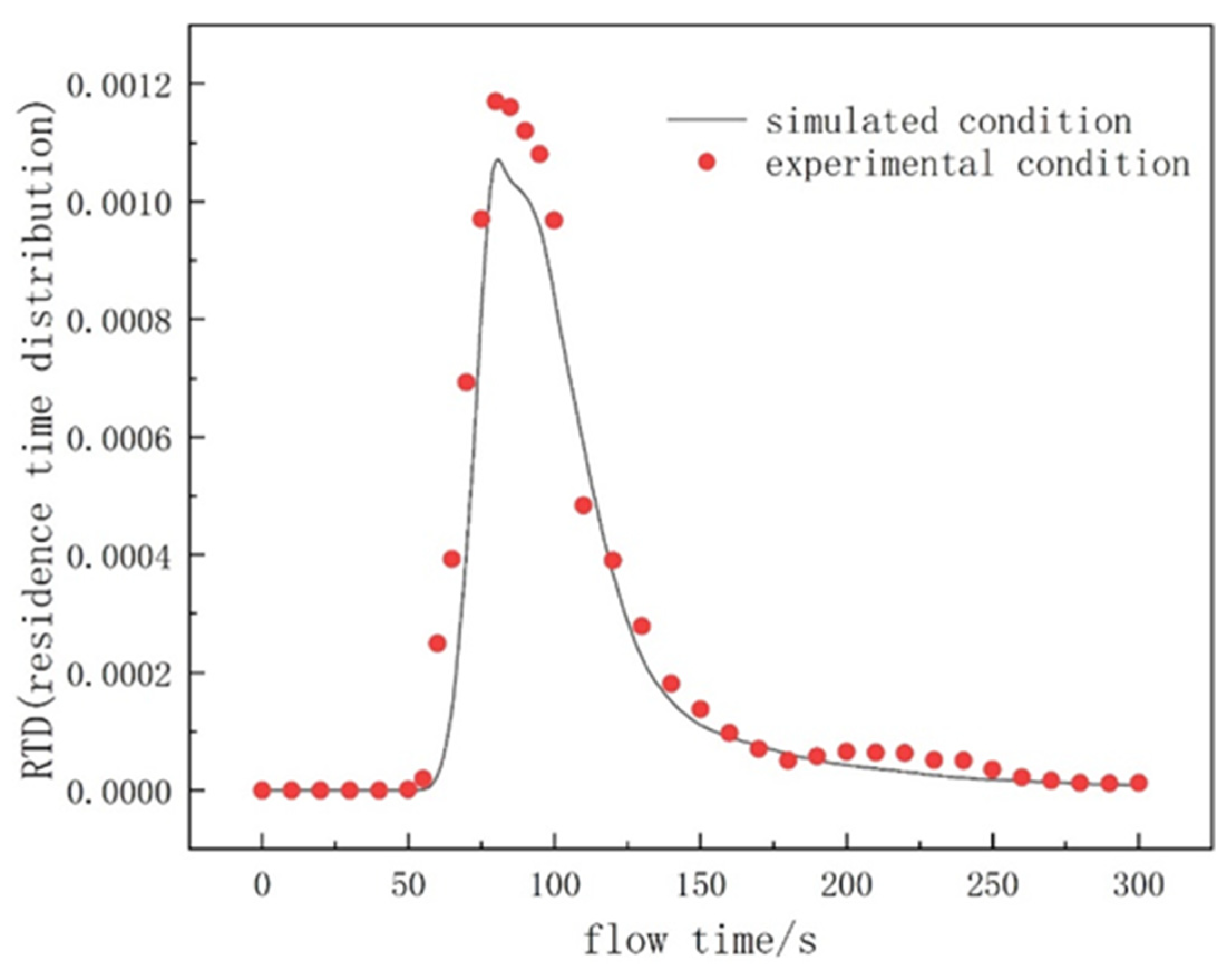
4.1. Comparative Analysis of Simulation Results and Experimental Results

Table 4. The change value of tracer concentration with time and residence time distribution density.

t/s	50	55	60	65	70	75	80	85	90	95	100
(c)p	1.25	4.73	66.13	44.67	101.58	100.42	77.50	73.38	55.88	37.38	17.23
E(t) × 104	0.01	0.19	2.49	3.92	6.93	9.70	11.70	11.60	11.20	10.80	9.68

shows the residence time distribution density of tracers in the experimental group within 50 s to 100 s, E(t) represents the residence time distribution density of tracer in the reactor. The formula of E(t) is shown below.

$$\mathrm{E}\left(\mathrm{t}\right)=\frac{V}{M}{\left(c\right)}_p=\frac{{\left(c\right)}_p}{{\int }_0^{300}{\left(c\right)}_{p}dt}$$

(6)

where (c)_p represents the concentration of tracer at the exit of pulse method; V is the tracer flow rate; M is the amount of tracer added in a very short instantaneous Δt time; t is sampling time.

Figure 10 shows the comparison of residence time distribution curves of tracers in the experimental group and the simulated group. The Figure 7 shows that simulation of tracer concentration change slightly slower than the response time of the experimental group, experimental group of tracer concentration peak in the 95 s, the error between the experimental and simulation data set is 8.2%, with the continuous decrease of tracer concentration, residence time distribution curve of the experimental and simulation group at the trailing approaching change trend, the error is reduced to within 3.3%. The residence time distribution density data of experimental group and simulation group are close, which verifies the correctness of the numerical model.

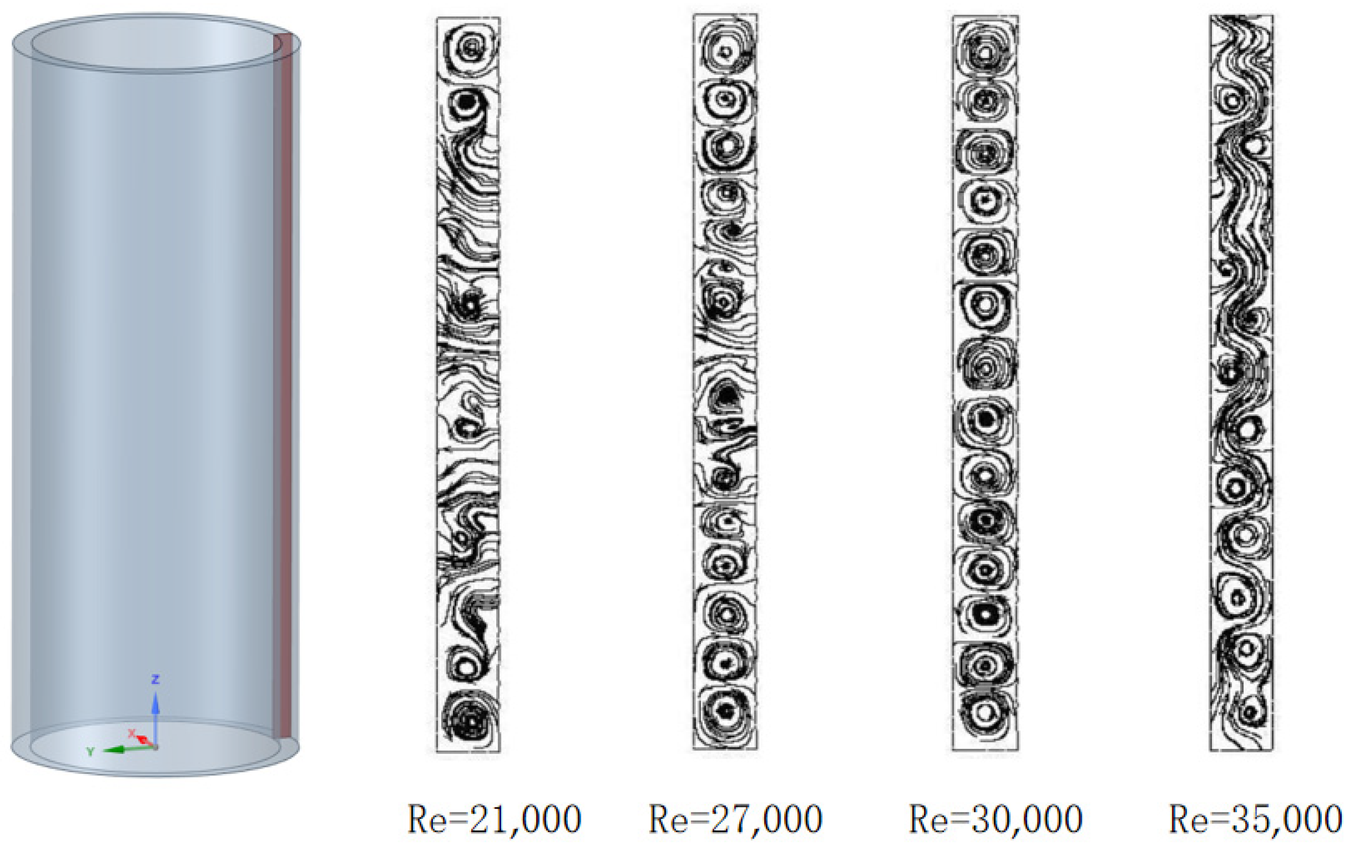
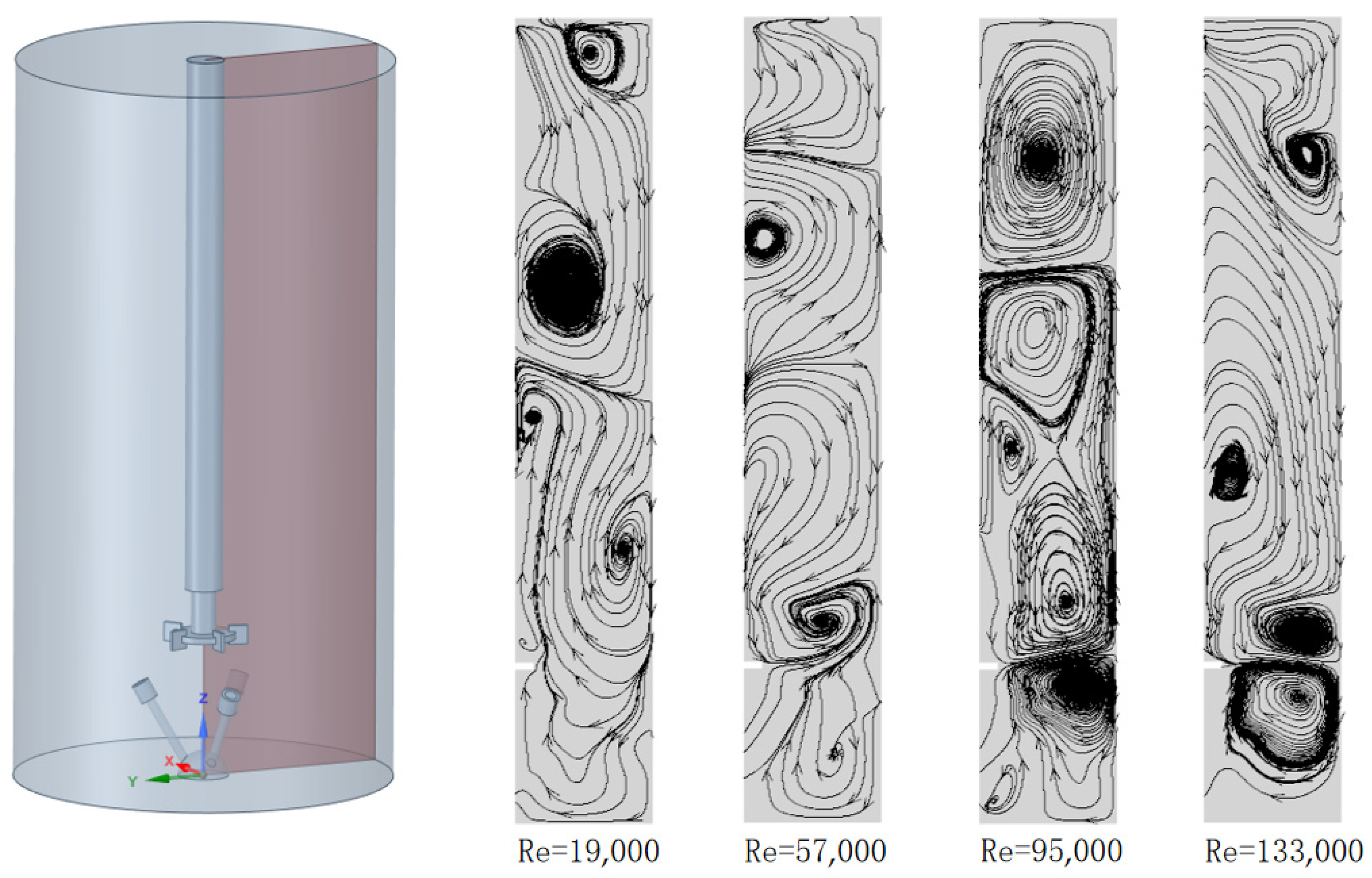
4.2. Influence of Taylor Vortex on Flow Field

Figure 11 shows the flow pattern evolution of Taylor vortex in the annulus (colored part) of a conventional Taylor flow reactor [27]. When the rotation Reynolds number is 21,000, the main stream region moves around the flow radially, a pair of relatively complete Taylor vortex cells appear at the top and bottom of the flow field and a small vortex core exists in the middle of the flow field, but the vortex cells are not formed yet. This is because the top and bottom walls have a large viscous force on the fluid and the end-wall effect is dominant compared with the centrifugal force, making the Taylor vortex appear at both ends of the walls first. With the increase of the rotating Reynolds number, the small vortex core region in the middle of the flow field is transformed into Taylor vortex cells. When the rotation Reynolds number reaches 30,000, the Taylor vortex cell of the flow field reaches the full vortex state and the Reynolds number at this time is called the critical rotation Reynolds number. As the number of rotating Reynolds continues to increase, Taylor vortex cells begin to break, evolve towards the wavy Taylor flow and eventually transition to turbulence.

Figure 12 shows the flow state evolution diagram of Taylor vortex in the axial section (colored part) of stirred tank Taylor flow reactor under different rotating Reynolds numbers. When the number of rotating Reynolds is 19,000, the main stream region splits into two counter-rotating vortices from the middle, and vortex core regions of different sizes appear. As the number of rotating Reynolds increases, the vortex core gradually evolves into a vortex cell. When the number of rotating Reynolds is 57,000, the evolution of the vortex core divides the flow field into multiple alternating vortex regions and gradually fills the annulus. When the rotating Reynolds number reaches 95,000, the vortex cell in the flow field reaches full vortex state. When the number of the rotating Reynolds continues to increase to 133,000, the vortex cell structure in the main stream area is destroyed and the flow field begins to evolve into wave flow.

By comparing Figure 11 and Figure 12, it can be seen that Taylor vortex is generated in stirred tank Taylor reactor by the introduction of gas distributor and its evolution law is consistent with that in conventional Taylor flow reactor.

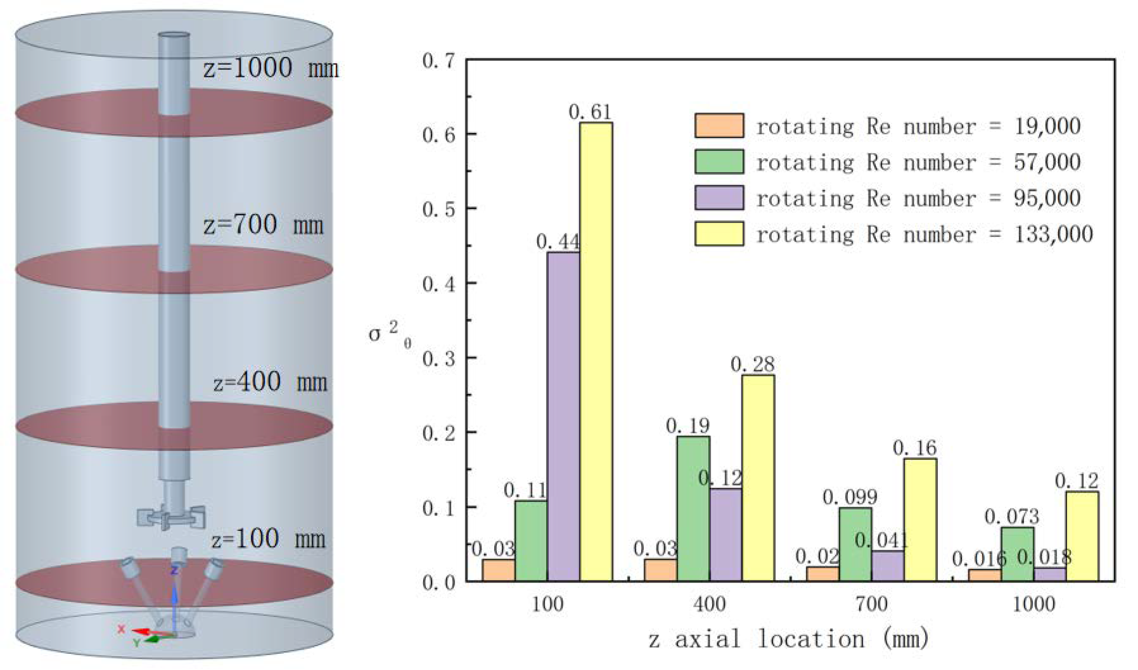
4.3. Influence of Taylor Vortex on Flow Model

The appearance of Taylor vortex changes the original flow pattern in stirred tank Taylor flow reactor and makes the flow field have unique macroscopic dynamic effect. The eigenvalue variance $\sigma$_θ² is used to quantify the flow model in the reactor, $\sigma$_θ² is the second moment of the average residence time of E(t) curve and is a measure of the dispersion degree of residence time distribution. The smaller $\sigma$_θ² is, the closer it is to the plug flow. When $\sigma$_θ² approaches 0, the flow pattern is close to plug flow and when $\sigma$_θ² approaches 1, the flow pattern is close to complete mixing flow [28]. The formula of $\sigma$_θ² is shown below.

$$t_m={\sum }_0^{300}{\left(c\right)}_{p}t/{\sum }_0^{300}{\left(c\right)}_p$$

(7)

$${\sigma }_{\theta }^2=\frac{\frac{{\sum }_0^{300}{t}^2{\left(c\right)}_p}{{\sum }_0^{300}{\left(c\right)}_p}-t_m^2}{t_m^2}$$

(8)

where $t_m$ represents the average residence time; and t is time from 0 to 300 s.

As can be seen from Figure 13, at the bottom of the reactor, as z = 100 mm, $\sigma$_θ² increases continuously from 0.03 to 0.61 with the increase of rotating Reynolds number. Combined with the analysis in Figure 9, it can be seen that the growth of Taylor vortex cell is limited in the bottom region of the reactor due to the lack of inductance of vortex flow at the inlet of the gas distributor. With the increase of impeller speed, the degree of fluid turbulence is gradually enhanced and the backmixing increases, making the flow in this region more and more close to the complete mixing flow.

In the region above the outlet of the gas distributor, the effect of increasing the number of rotating Reynolds on $\sigma$_θ² is different from that at the bottom of the reactor. At low rotational Reynolds number (Re = 19,000), $\sigma$_θ² is less than 0.03 at z = 400 mm, z = 700 mm and z = 1000 mm sections. The low rotational Reynolds number causes insufficient driving force, resulting in insufficient fluid mixing. When the rotation Reynolds number increases from 19,000 to 57,000, the $\sigma$_θ² value continues to increase, indicating that the mixing effect between the fluids is strengthened, the backmixing becomes larger and the flow pattern develops to the direction of complete mixing flow. When the rotation Reynolds number is close to the critical value, the trend of $\sigma$_θ² decreases with the increase of rotation Reynolds number, this is because in the complete mixing flow region generated by strong agitation, Taylor vortex cells formed a local plug flow region, which reduced the backmixing in the reactor and$\sigma$_θ². When the Reynolds number reaches the critical value, the $\sigma$_θ² value increases again and the structure of the Taylor vortex is destroyed at high rotational speed and the backmixing is strengthened again.

4.4. Influence of Taylor Vortex on Mass Transfer

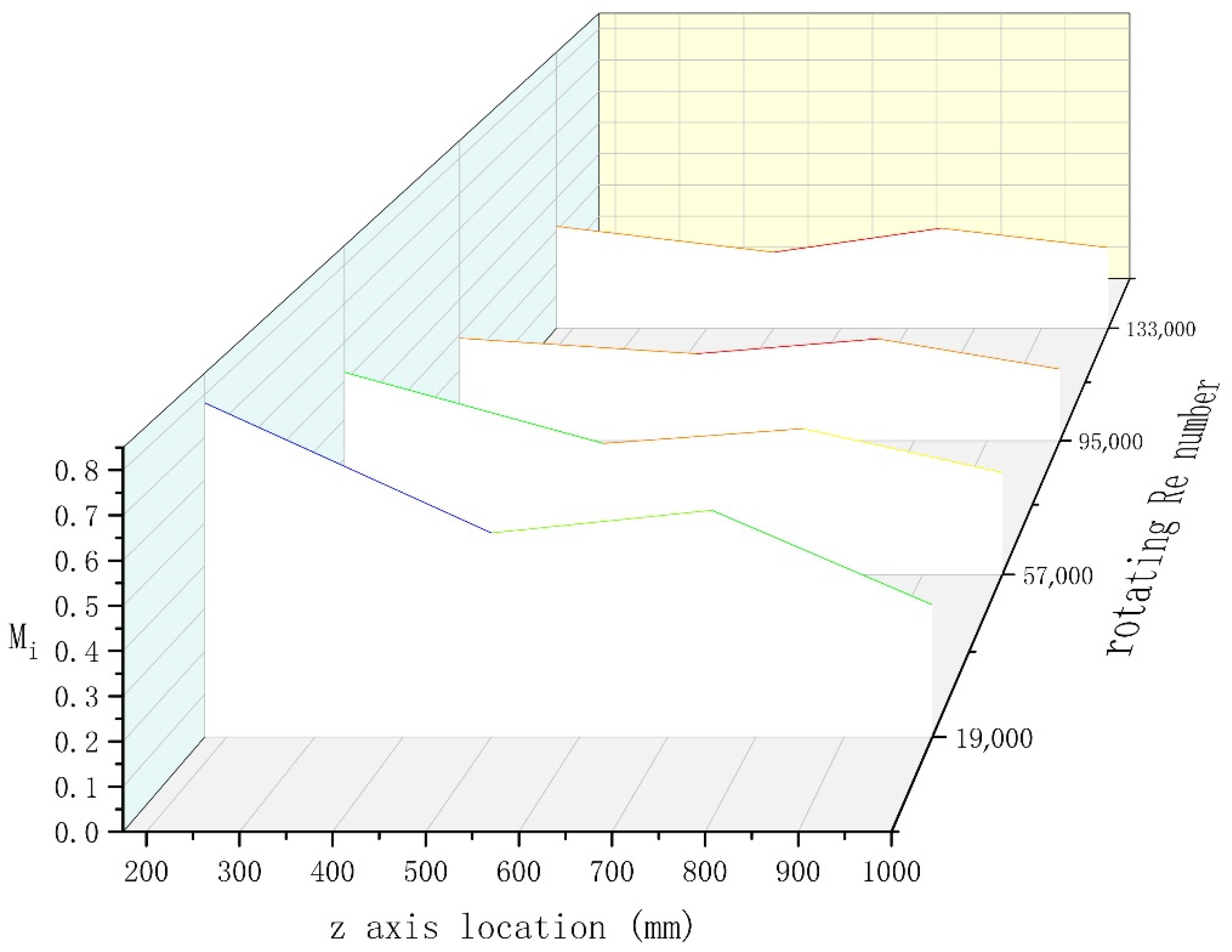
4.4.1. Influence of Taylor Vortex on Gas Phase Homogeneity

At cross sections z = 100 mm, z = 400 mm, z = 700 and z = 1000 mm away from the bottom of the reactor, six straight lines are obtained at an angle of 30°, twenty gas phase velocity monitoring points are taken from each line and a total of 120 monitoring points are taken from each cross section. The gas phase homogeneity coefficient Mi is used to represent the gas phase homogeneity. The smaller Mi is, the better the gas phase homogeneity performance [29].

$$M_i=\sqrt{\frac{1}{N}{\displaystyle \sum _{j=1}^N{(\frac{u_j-u}{u})}^2}}$$

(9)

where N is the total number of gas phase monitoring points; U_j is the gas phase velocity at each monitoring point; U is the plane average gas phase velocity.

Figure 14 shows Mi at different heights under different rotation Reynolds numbers. In other words, the larger the number of rotating Reynolds is, the better the gas phase homogeneity is. When the critical number of rotating Reynolds is 95,000, the Mi at z = 1000 mm reaches the minimum value 0.2 and the overall gas phase homogeneity in the reactor is the best. Compared with the number of rotating Reynolds is 57,000, the gas phase homogeneity increases by about 28%.

At different heights under the same rotation Reynolds number, Mi at the bottom, z = 100 mm, is much larger than Mi at the middle and upper parts. When Reynolds reaches 19,000, the Mi value at z = 100 mm is as high as 0.78, which is due to the lack of cyclone induction and the small stirring effect, making the gas phase homogeneity in this region the worst. The cross sections at z = 700 mm are located between two adjacent Taylor vortex cells with opposite rotations, while the cross sections at z = 400 mm and 1000 mm are respectively located near Taylor vortex cores. As can be seen from Figure 14, under the same rotation Reynolds number, the Mi values at z = 700 mm are larger than those of the other two cross sections. The mixing effect between vortex cells is not as strong as that at vortex core. The distribution of Taylor vortex cells plays a decisive role in the diffusion of gas phase in liquid phase.

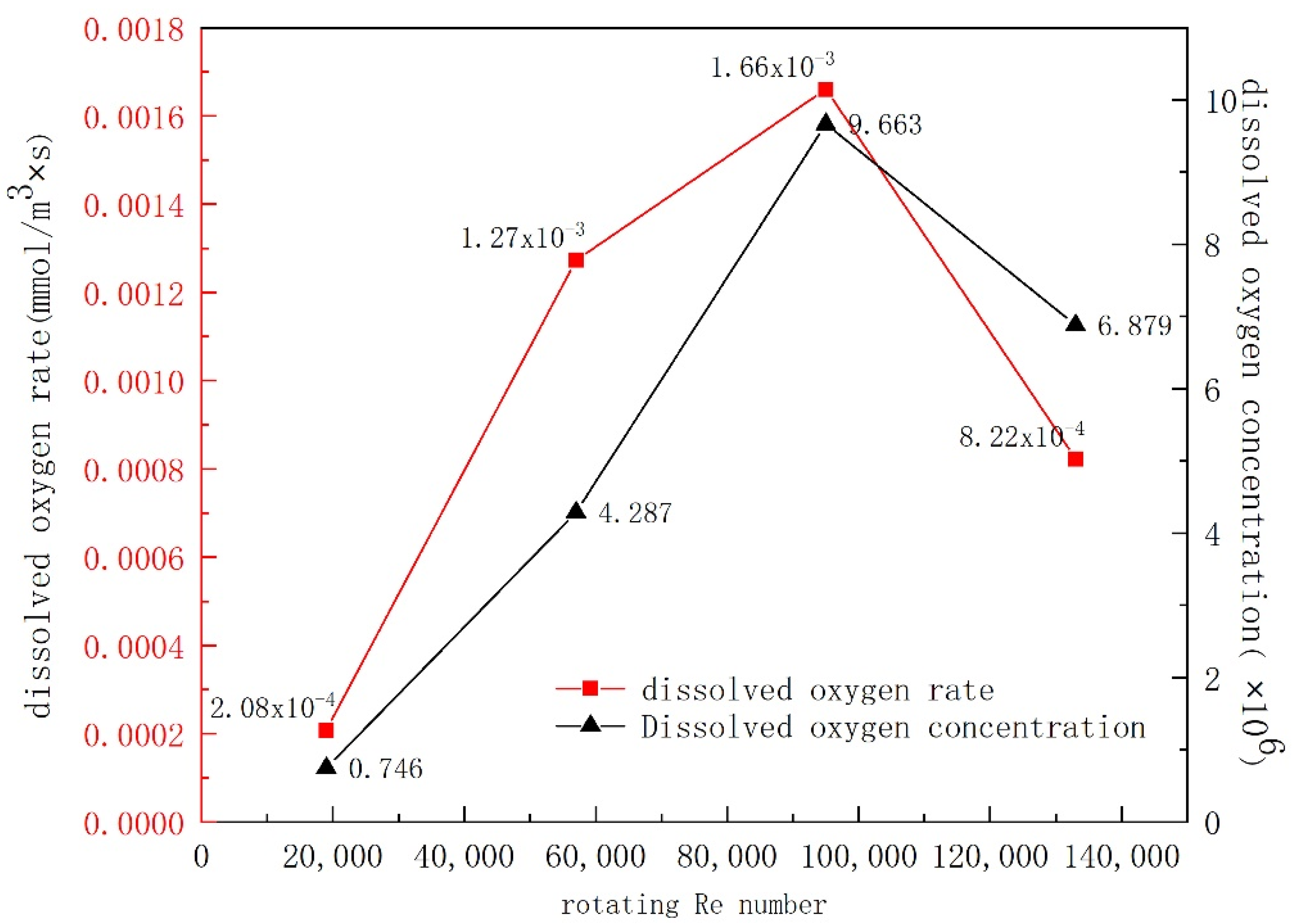
4.4.2. Influence of Taylor Vortex on Dissolved Oxygen

Figure 15 shows the overall dissolved oxygen rate of the reactor and the dissolved oxygen in the liquid phase under different rotating Reynolds numbers. As can be seen from the figure, before the critical rotation Reynolds number is reached, the dissolved oxygen rate and liquid phase dissolved oxygen increase with the increase of rotation Reynolds number until the full vortex structure is reached. When the number of rotating Reynolds increases from 19,000 to 57,000, the increase trend is most obvious and the dissolved oxygen rate increases from 2.08 × 10⁻⁴ mmol/m³.s to 1.27 × 10⁻³ mmol/m³.s rapidly, which is about 5 times higher, and the dissolved oxygen in liquid phase also increases correspondingly from 0.746 × 10⁻⁶ to 9.663 × 10⁻⁶.

When the rotational Reynolds number reaches the critical value and continues to increase, the dissolved oxygen rate decreases from 1.66 × 10⁻³ mmol/m³·s to 8.22 × 10⁻⁴ mmol/m³·s, due to the destruction of Taylor vortex cell structure and the enhance of backmixing, the dissolved oxygen rate also decreases correspondingly.

From the above analysis, it can be seen that in the process of Taylor vortex cell forming and evolving to full vortex, the existence of vortex cell has a positive effect on oxygen transfer rate between gas and liquid phase, while when the full vortex structure is destroyed and the flow evolves to a wavy Taylor flow, the mass transfer effect of dissolved oxygen is weakened. In addition, the gas–liquid mixed jet emitted by the gas distributor is broken into small bubbles under the shear action of the blade. The bubble size decreases with the increase of the stirring speed, which is also conducive to the process of dissolved oxygen.

5. Conclusions

In this paper, Taylor vortex is generated in the stirred tank Taylor reactor by installing a gas distributor at the bottom of the reactor. Numerical simulation and experimental study are used to study the characteristics of the flow field in the reactor under different rotating Reynolds numbers and the existence of Taylor vortex is verified. Combining the variance of residence time distribution density with the flow pattern, the flow model in the reactor was quantitatively analyzed. Taking gas phase homogeneity, dissolved oxygen rate and dissolved oxygen as objects, the strengthening effect of Taylor vortex on mass transfer was studied and the following conclusions are drawn:

(1)

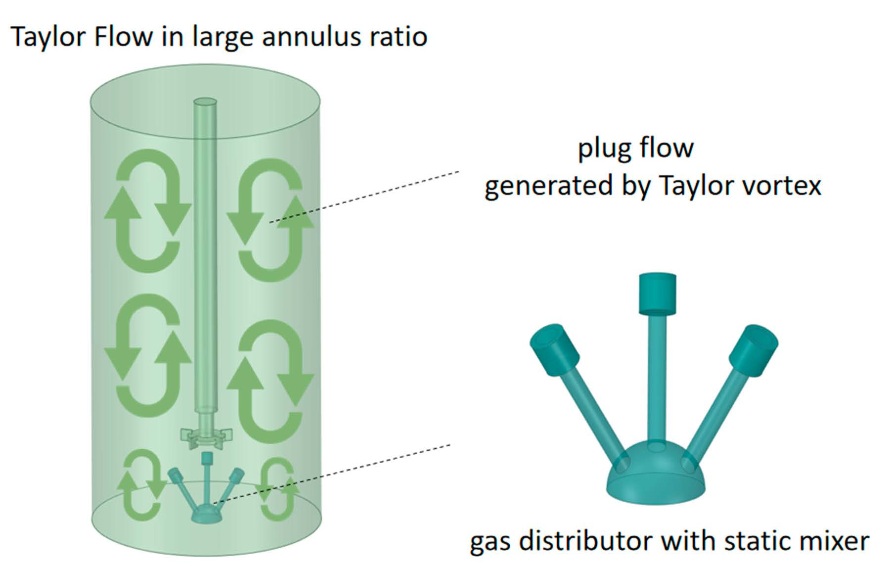
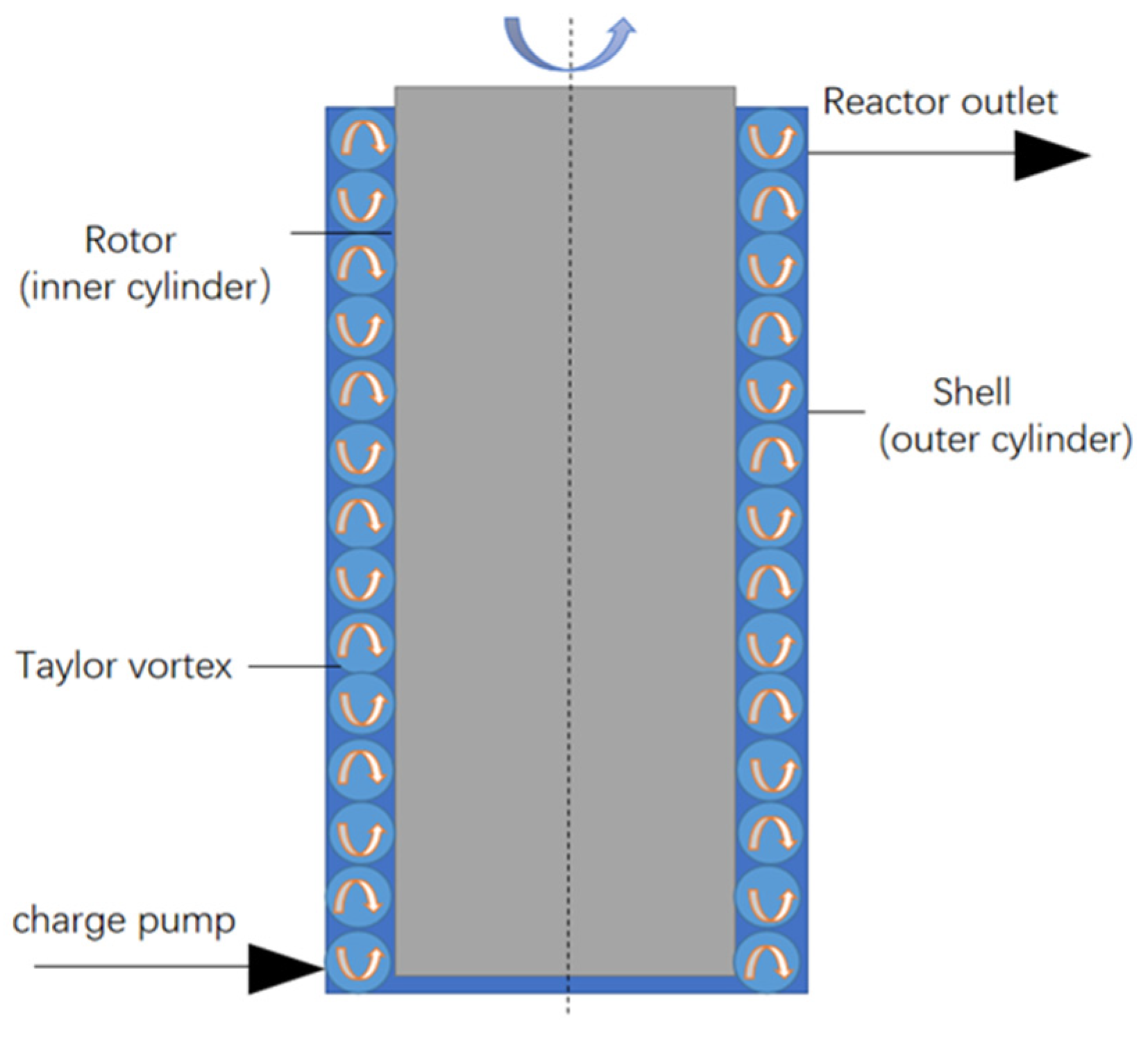
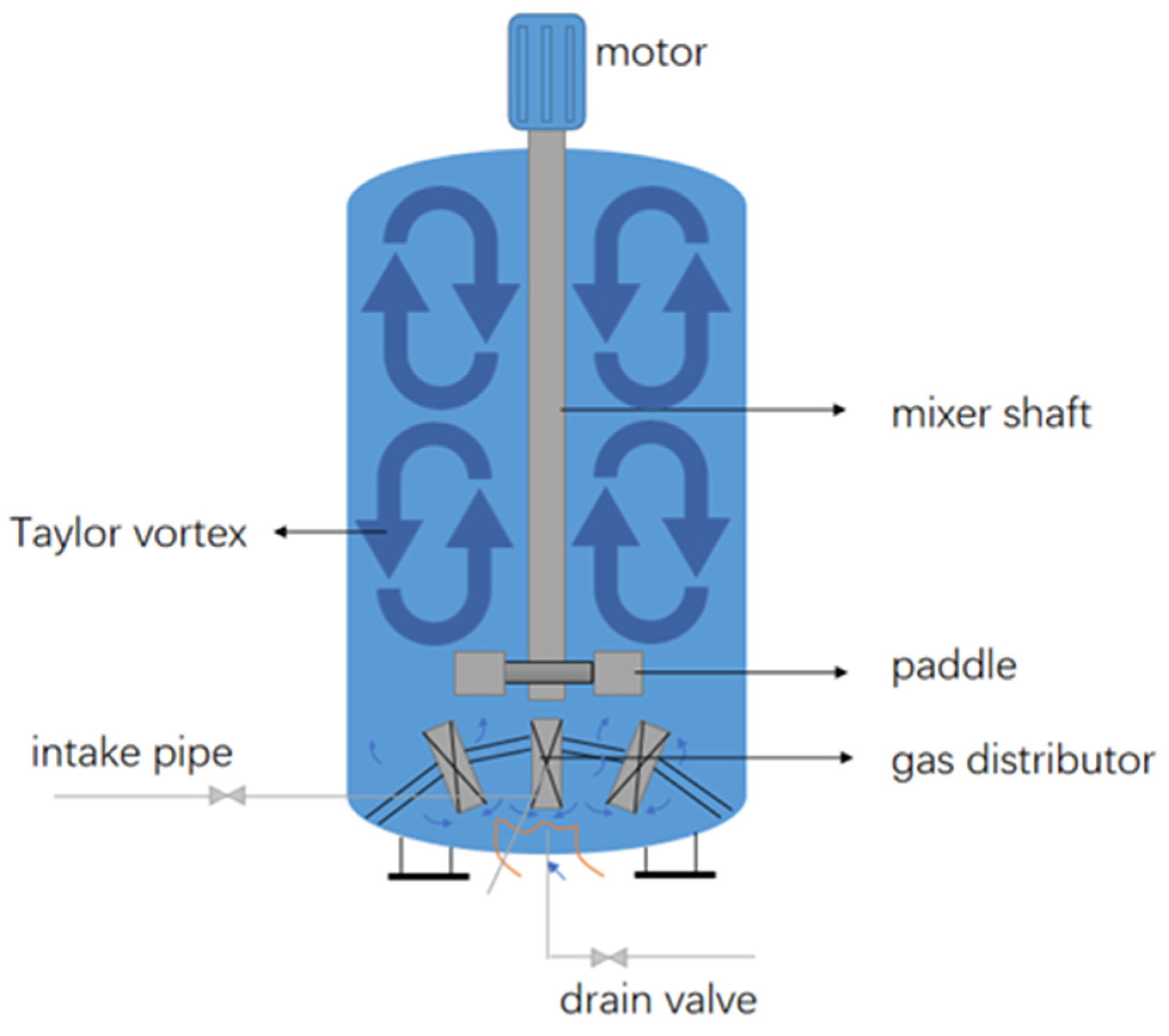
Taylor vortex is formed in stirred tank Taylor reactor by gas distributor and its evolution law is consistent with that in conventional Taylor flow reactor.

(2)

The effect of increasing rotation Reynolds number on the difference eigenvalue variance $\sigma$_θ² is different in the region above the outlet of the gas distributor and in the region at the bottom of the reactor. The stirring action of the impeller leads to the enhancement of backmixing, while the Taylor vortex will build up a local plug flow area in the reactor, which reduces backmixing.

(3)

Under the critical Reynolds number Re_cr, the gas phase homogeneity of the reactor is increased by about 28% compared with the low rotation Reynolds number and the dissolved oxygen rate is increased by about 5 times, which effectively improves the flow condition in the reactor and strengthens the mass transfer efficiency between gas and liquid.

(4)

The variation trend of residence time distribution curves obtained by experiment and numerical simulation is consistent and the error between experimental data and simulated data is no more than 8.2%, which verifies the correctness of the numerical model.

References

1. Singh, R.S.; Singh, T.; Pandey, A. Production of fungal endoinulinase in a stirred tank reactor and fructooligosaccharides preparation by crude endoinulinase. Bioresour. Technol. Rep. 2021, 15, 388–395. [Google Scholar] [CrossRef]
2. Wang, Z.; Zeng, J. Application of moving horizon estimation in continuous stirred tank reactors. Comput. Appl. Softw. 2021, 38, 67–71. [Google Scholar]
3. Abiev, R.S. Gas-liquid and gas-liquid-solid mass transfer model for Taylor flow in micro (milli) channels: A theoretical approach and experimental proof. Chem. Eng. J. Adv. 2020, 4, 1875–1882. [Google Scholar] [CrossRef]
4. Dong, S.; Ji, X.-Y.; Li, C.-X. Large eddy simulation of Taylor-Couette turbulent flow under transverse magnetic field. Acta Phys. Sin. 2021, 70, 216–224. [Google Scholar] [CrossRef]
5. Lim, J.G.; Yoon, S.H.; Hong, J.; Choi, J.B.; Kim, M.K.; Lee, T.R. Continuous synthesis of nickel/cobalt/manganese hydroxide microparticles in Taylor–Couette reactors. J. Ind. Eng. Chem. 2021, 99, 388–395. [Google Scholar] [CrossRef]
6. Hosoya, M.; Manaka, A.; Nishijima, S.; Tsuno, N. Development of a Liquid-Liquid Biphasic Reaction Using a Taylor Vortex Flow Reactor. Asian J. Org. Chem. 2021, 10, 1414–1418. [Google Scholar] [CrossRef]
7. Kaye, J.; Elgar, E. Modes of adiabatic and diabatic fluid flow in an annulus with an inner rotating cylinder. Trans. ASME 1958, 80, 753–765. [Google Scholar] [CrossRef]
8. Gil, L.V.G.; Singh, H.; da Silva, J.D.S.; dos Santos, D.P.; Covas, D.T.; Swiech, K.; Suazo, C.A.T. Feasibility of the taylor vortex flow bioreactor for mesenchymal stromal cell expansion on microcarriers. Biochem. Eng. J. 2020, 162, 107710. [Google Scholar]
9. Sha, Y.; Fritz, J.; Klemm, T.; Ripperger, S. Untersuchung der Strömung im Taylor-Couette-System bei geringen Spaltbreiten. Chem. Ing. Tech. 2016, 88, 640–647. [Google Scholar] [CrossRef]
10. Yin, J.; Liu, X.; Zhou, C.; Zhu, Z. Analysis and measurement of mixing flow field on side wall of large-scale mixing tank. Chem. Eng. 2021, 49, 73–78. [Google Scholar]
11. Zhu, J.; Liu, D.; Tang, C.; Chao, C.Q.; Wang, C.L. Study of Slit Wall Aspect Ratio Effect on the Taylor Vortex Flow. J. Eng. Thermophys. 2016, 37, 1208–1211. [Google Scholar]
12. Lei, M.; Li, M. High-Performance Manufacturing Principle and Application of Thrust Bearings of Primary Pump in Nuclear Power Plant. China Nucl. Power 2020, 13, 592–598. [Google Scholar]
13. Giordano, R.C.; Giordano, R.L.C.; Prazeres, D.M.F.; Cooney, C.L. Analysis of a Taylor–Poiseuille vortex flow reactor—I: Flow patterns and mass transfer characteristics. Chem. Eng. Sci. 1998, 53, 3635–3652. [Google Scholar] [CrossRef]
14. Giordano, R.L.C.; Giordano, R.C.; Prazeres, D.M.F.; Cooney, C.L. Analysis of a Taylor–Poiseuille vortex flow reactor—II: Reactor modeling and performance assessment using glucose-fructose isomerization as test reaction. Chem. Eng. Sci. 2000, 55, 3611–3626. [Google Scholar] [CrossRef]
15. Resende, M.M.; Tardioli, P.W.; Fernandez, V.M.; Ferreira, A.L.O.; Giordano, R.L.C.; Giordano, R.C. Distribution of suspended particles in a Taylor–Poiseuille vortex flow reactor. Chem. Eng. Sci. 2001, 56, 755–761. [Google Scholar] [CrossRef]
16. Resende, M.M.; Vieira, P.G.; Sousa, R., Jr.; Giordano, R.L.C.; Giordano, R.C. Estimation of mass transfer parameters in a Taylor-Couette-Poiseuille heterogeneous reactor. Braz. J. Chem. Eng. 2004, 21, 175–184. [Google Scholar] [CrossRef]
17. Ostilla-Mónico, R.; Van der Poel, E.; Verzicco, R.; Grossmann, S.; Lohse, D. Exploring the phase diagram of fully turbulent Taylor–Couette flow. J. Fluid Mech. 2014, 761, 1–26. [Google Scholar] [CrossRef] [Green Version]
18. Richter, O.; Menges, M.; Kraushaar-Czarnetzki, B. Investigation of mixing in a rotor shape modified Taylor-vortex reactor by the means of a chemical test reaction. Chem. Eng. Sci. 2009, 64, 2384–2391. [Google Scholar] [CrossRef]
19. Deng, R.; Arifin, D.Y.; Chyn, M.Y.; Wang, C.H. Taylor vortex flow in presence of internal baffles. Chem. Eng. Sci. 2010, 65, 4598–4605. [Google Scholar] [CrossRef]
20. Carlos Álvarez, M.; Vicente, W.; Solorio, F.; Mancilla, E.; Salinas, M.; Zenit, V.R. A study of the Taylor-Couette flow with finned surface rotation. J. Appl. Fluid Mech. 2019, 12, 1371–1382. [Google Scholar] [CrossRef]
21. Yang, G.; Wang, M. Numerical simulation and performance analysis of flow field in coaxial contra-rotating bioreactor. CIESC J. 2020, 71, 5188–5199. [Google Scholar]
22. Berghout, P.; Dingemans, R.J.; Zhu, X.; Verzicco, R.; Stevens, R.J.; Van Saarloos, W.; Lohse, D. Direct numerical simulations of spiral Taylor–Couette turbulence. J. Fluid Mech. 2020, 887, 18. [Google Scholar] [CrossRef] [Green Version]
23. Bakhuis, D.; Ezeta, R.; Berghout, P.; Bullee, P.A.; Tai, D.; Chung, D.; Verzicco, R.; Lohse, D.; Huisman, S.G.; Sun, C. Controlling secondary flow in Taylor–Couette turbulence through spanwise-varying roughness. J. Fluid Mech. 2019, 883, 654–662. [Google Scholar] [CrossRef] [Green Version]
24. Qin, Z.; Zhang, Q.; Liu, Y.; Guo, J.; Shi, Y. PIV measurement and CFD simulation of flow characteristic in a spinning disc reactor. Chem. Eng. 2019, 47, 44–49. [Google Scholar]
25. Hiroyuki, F.; Noritaka, S. Velocity Component Comparison between CFD and EFD in Taylor Vortex Flow. J. Mech. Eng. Autom. 2017, 7, 327–334. [Google Scholar] [CrossRef] [Green Version]
26. Ma, R.-X.; Wang, Y.-M.; Zhang, S.-H.; Wu, C.-H.; Wang, X.-N. Numerical investigation of scale effect on acoustic scattering by vortex. Acta Phys. Sin. 2021, 70, 184–193. [Google Scholar] [CrossRef]
27. Ye, L.; Li, L.N.; Chen, D.; Xie, F. Flow and reaction performance of Taylor-vortex flow reactor. CIESC J. 2013, 64, 2058–2064. [Google Scholar]
28. Karen, L.; Henderson, D.; Rhys, G. Limiting behavior of particles in Taylor-Couette flow. J. Eng. Math. 2010, 67, 85–94. [Google Scholar]
29. Hiroyuki, F. Interactive Visualization System of Taylor Vortex Flow Using Stokes’ Stream Function. World J. Mech. 2012, 2, 188–196. [Google Scholar]
Figure 1. Schematic diagram of conventional Teller reactor.
Energies 15 02028 g001
Figure 2. Schematic diagram of stirred tank Taylor reactor.
Energies 15 02028 g002
Figure 3. Schematic diagram of experimental device. 1 turbulence pump; 2 air pipe; 3 drain valve; 4 gas distributor; 5 stirring blade; 6 shaft; 7 electromotor; 8 frequency changer; 9 power supply; 10 light source;11 digital camera; 12 computer.
Energies 15 02028 g003
Figure 4. Schematic diagram of spectrophotometer and samples.
Energies 15 02028 g004
Figure 5. Geometric model of stirred tank Taylor reactor.
Energies 15 02028 g005
Figure 6. Schematic diagram of gas distributor.
Energies 15 02028 g006
Figure 7. Volume mesh on Y = 0 clipping plane.
Energies 15 02028 g007
Figure 8. Grid independence verification curve.
Energies 15 02028 g008
Figure 9. Boundary conditions and cell zones of the domain.
Energies 15 02028 g009
Figure 10. Comparison of residence time distribution curves.
Energies 15 02028 g010
Figure 11. Annulus flow diagram of conventional Taylor reactor.
Energies 15 02028 g011
Figure 12. Annulus flow diagram of stirred tank Taylor reactor.
Energies 15 02028 g012
Figure 13. Variances under different rotation Reynolds numbers.
Energies 15 02028 g013
Figure 14. Gas phase homogeneity at different heights.
Energies 15 02028 g014
Figure 15. The dissolved oxygen rate and liquid oxygen content of the reactor under different rotating Re numbers.
Energies 15 02028 g015