
Optimal Operation for Regional IES Considering the Demand- and Supply-Side Characteristics


Abstract
:1. Introduction
1.1. Motivation
1.2. Previous Work
1.3. Current Contribution
- (1)
- An alliance strategy for energy-consuming entities in a CIES is proposed on the basis of social network theory, which can simplify the number of transaction objects while considering the coupling relationship on the demand side.
- (2)
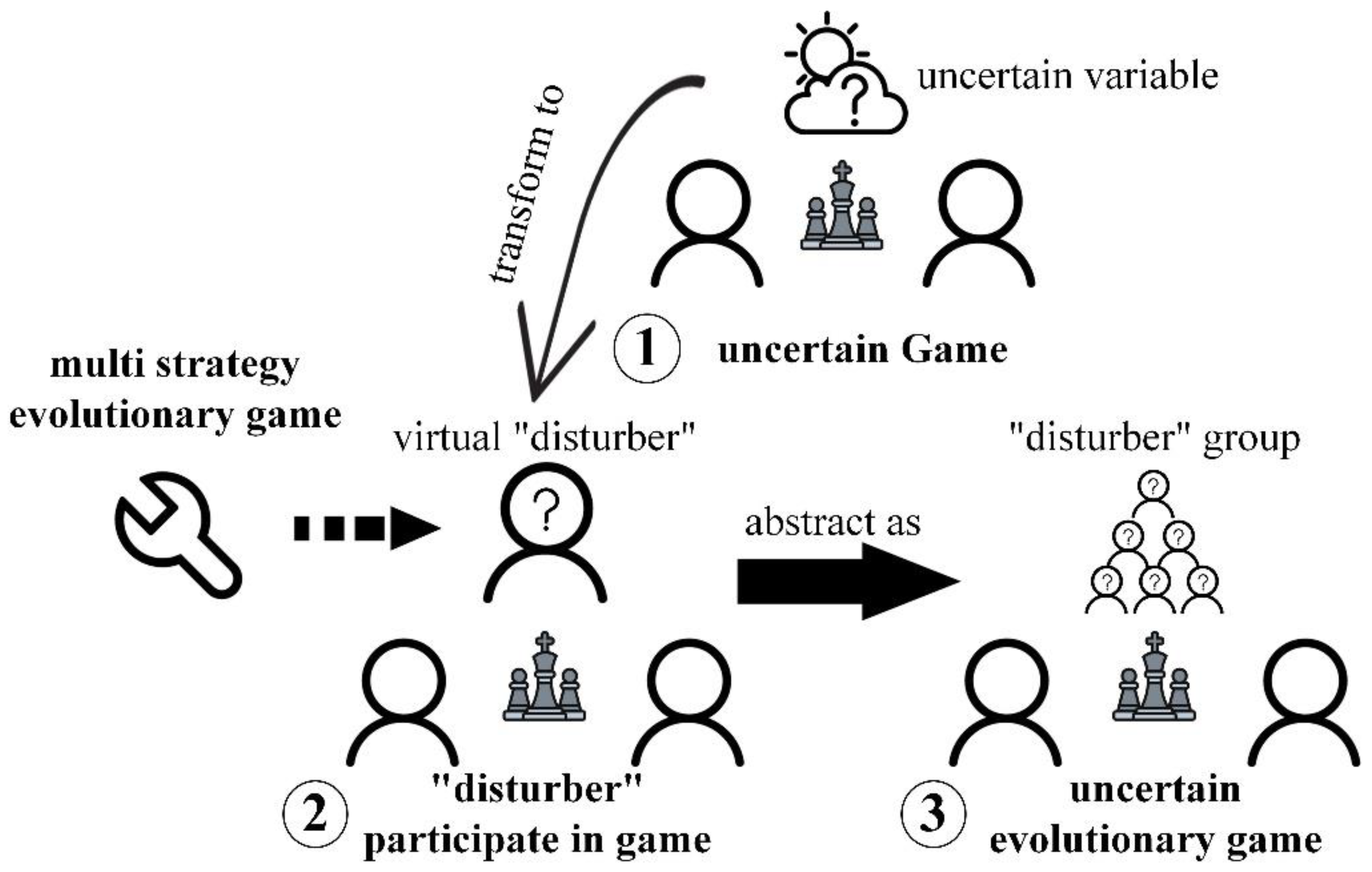
- A distributed PV output characteristic model based on the uncertain evolutionary game method is constructed, which fully considers the risk cost on the supply side and the impact of the uncertainty output on the trading strategy.
- (3)
- Considering the uncertainty of distributed photovoltaic output and the energy-consumption interactions, an optimal operation method for RIES based on social network theory and the uncertain evolutionary game method is proposed in this paper.
- (4)
- A case study is carried out for an RIES consisting of three CIESs; the results show that the proposed method can ensure a reasonable distribution of benefits for each participant, while having great significance for optimizing the energy composition and promoting the local consumption of renewable energy.
1.4. Structure
2. Characteristic Modeling of Community Energy-Consuming Entities Based on Social Network Theory
2.1. Social Network Theory
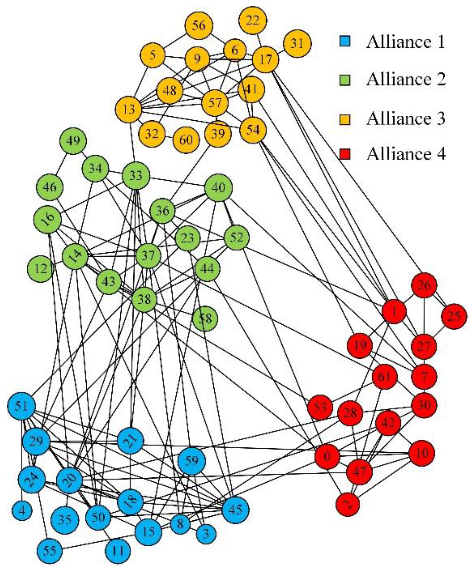
2.2. Alliance Strategy for Community Energy-Consuming Entities
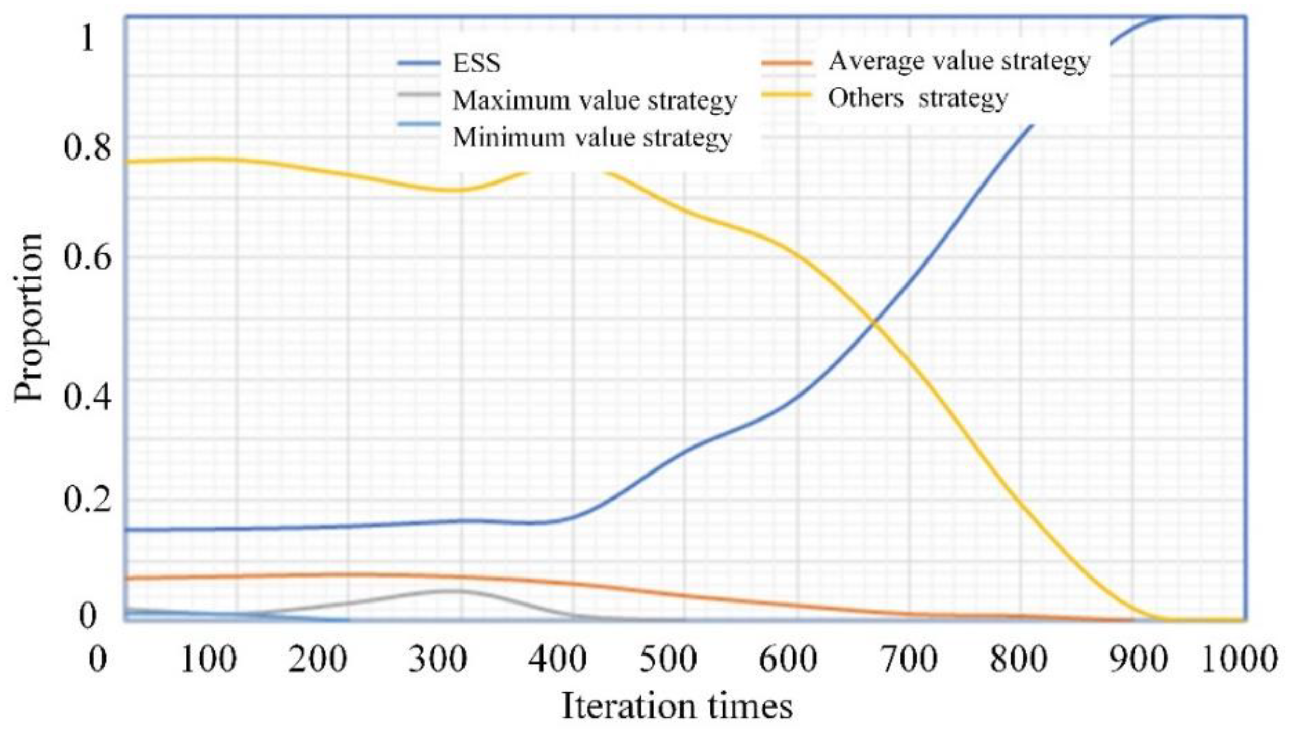
3. Characteristic Modeling of Distributed Photovoltaic Output Based on Uncertain Evolutionary Game
3.1. Uncertain Evolutionary Game
3.2. Characteristic Model of Distributed Photovoltaic Output
4. Optimal Operation Strategy for Regional Integrated Energy System
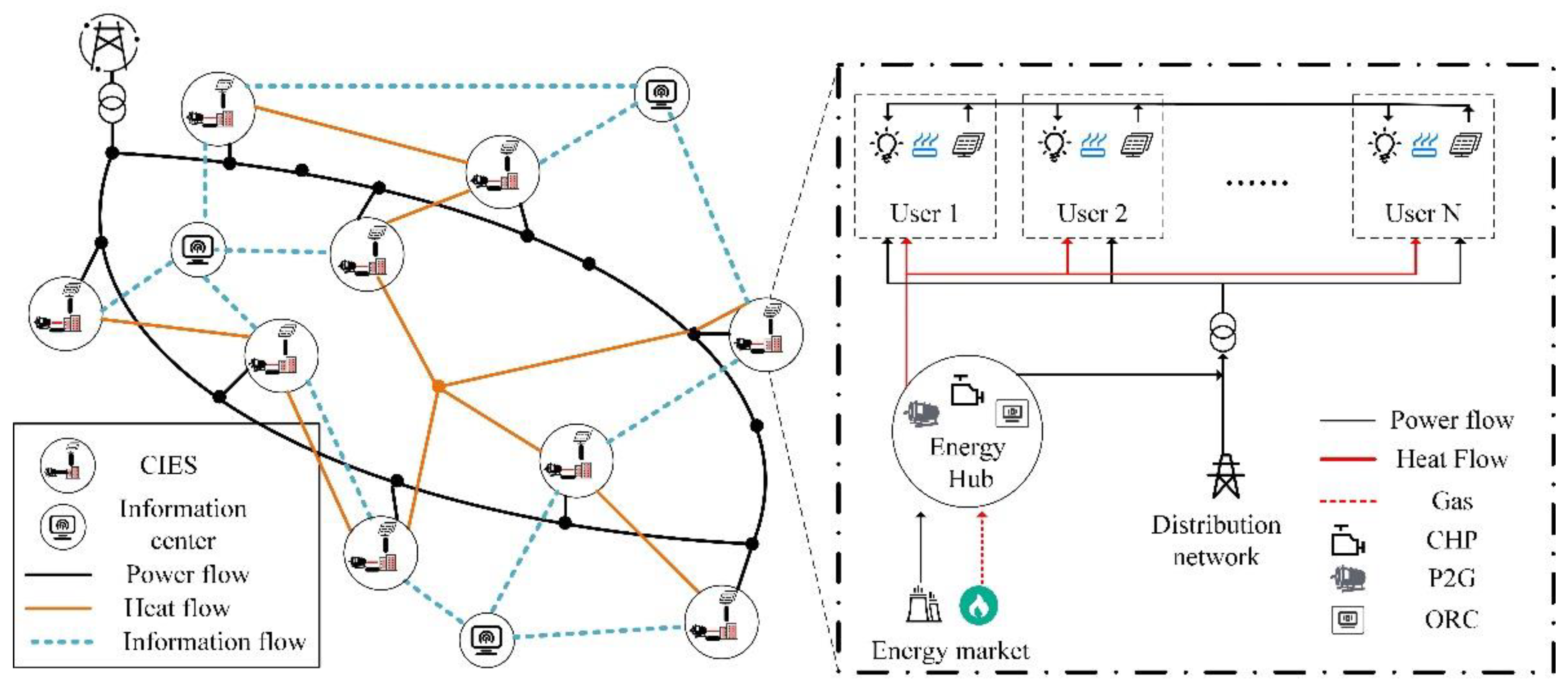
4.1. Regional Integrated Energy System Structure
4.2. Energy-Consumption and Profit Models
4.2.1. Energy-Consumption Model
4.2.2. Profit Model
4.3. Energy Flow and Profit Model
4.3.1. Energy Flow Model
4.3.2. Profit Model
4.4. Energy System and Operator Profit Models
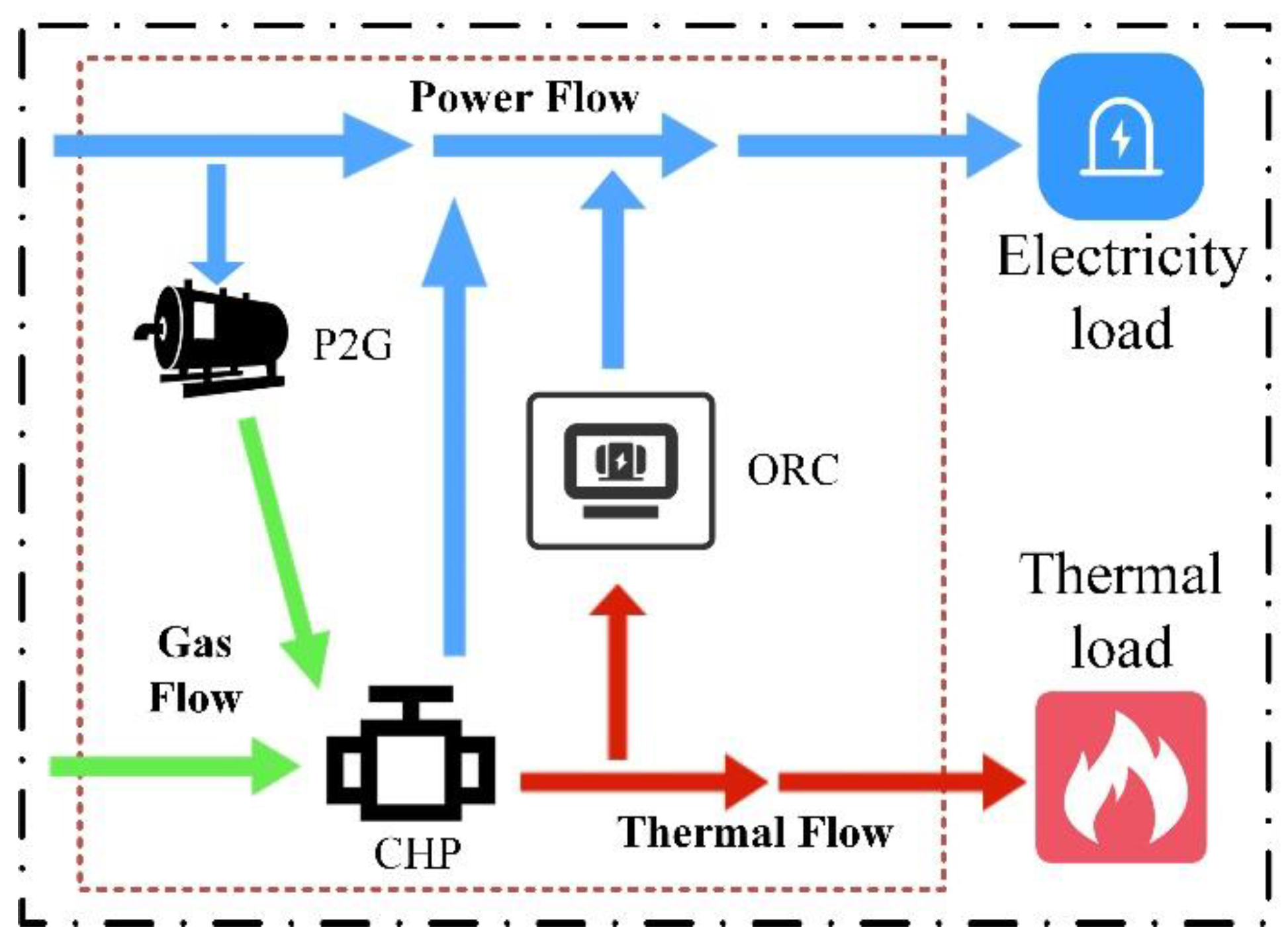
4.4.1. Energy System Model
- (1)
- Power-to-gas equipment
- (2)
- Combined heat and power unit
- (3)
- Waste heat power generation system
- (4)
- Energy hub model
4.4.2. Operator Profit Model
- (1)
- Profit model
- (2)
- Cost model
4.5. Optimal Operation Strategy
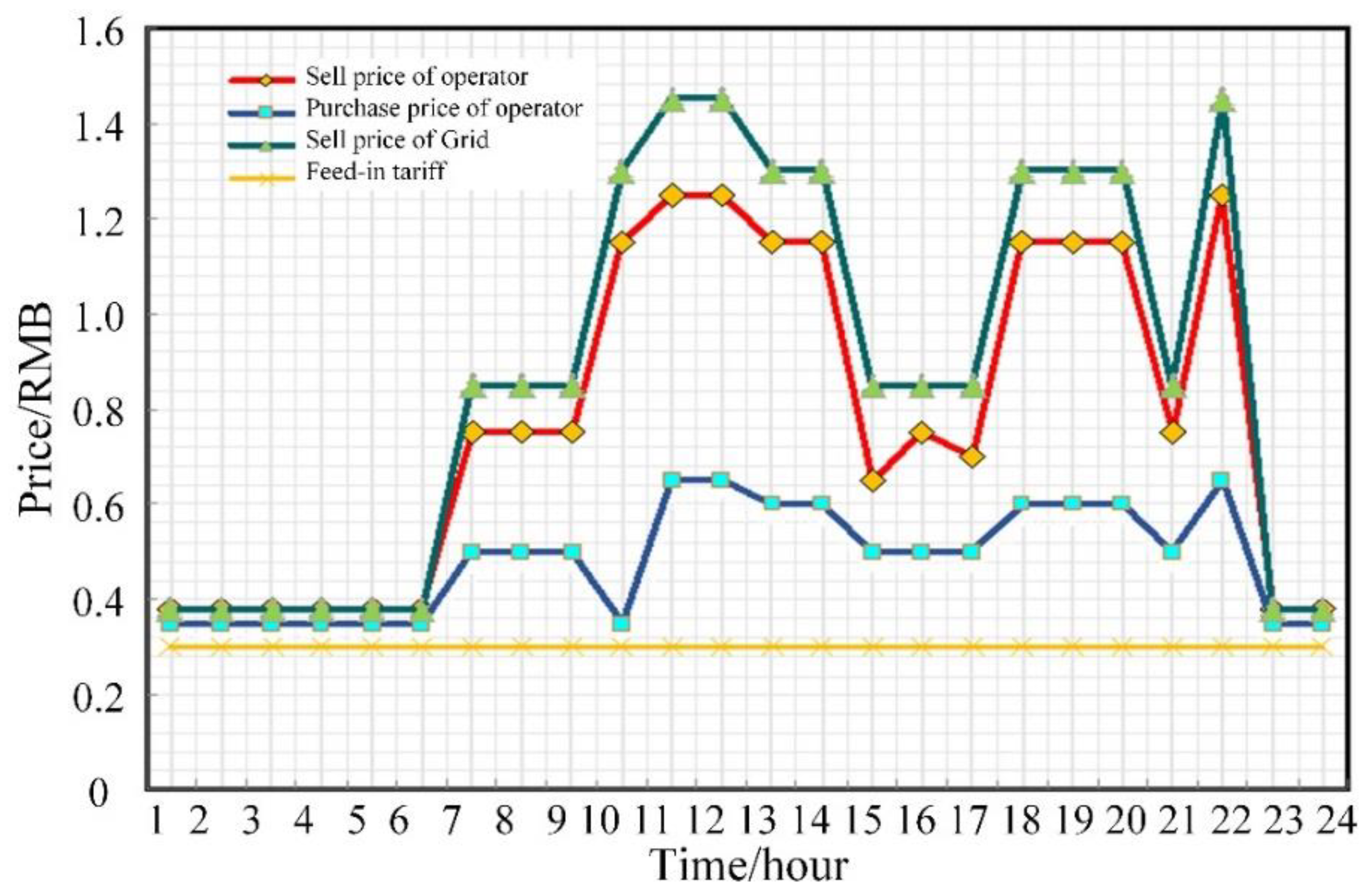
4.5.1. Energy Transaction Strategy of Community-Integrated Energy System
4.5.2. Optimal Operation Strategy for Regional Integrated Energy System
5. Case Study
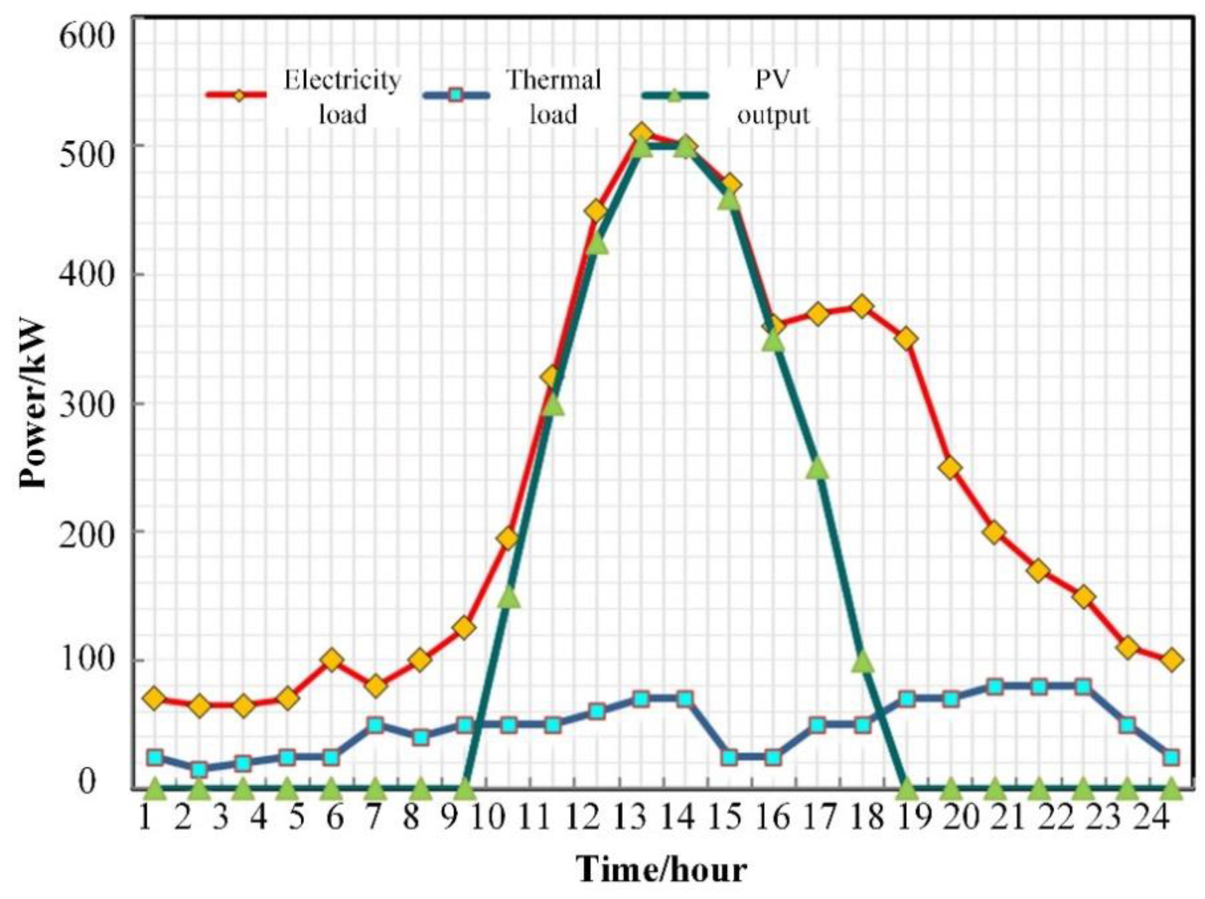
5.1. Case Description
5.2. Results and Discussion
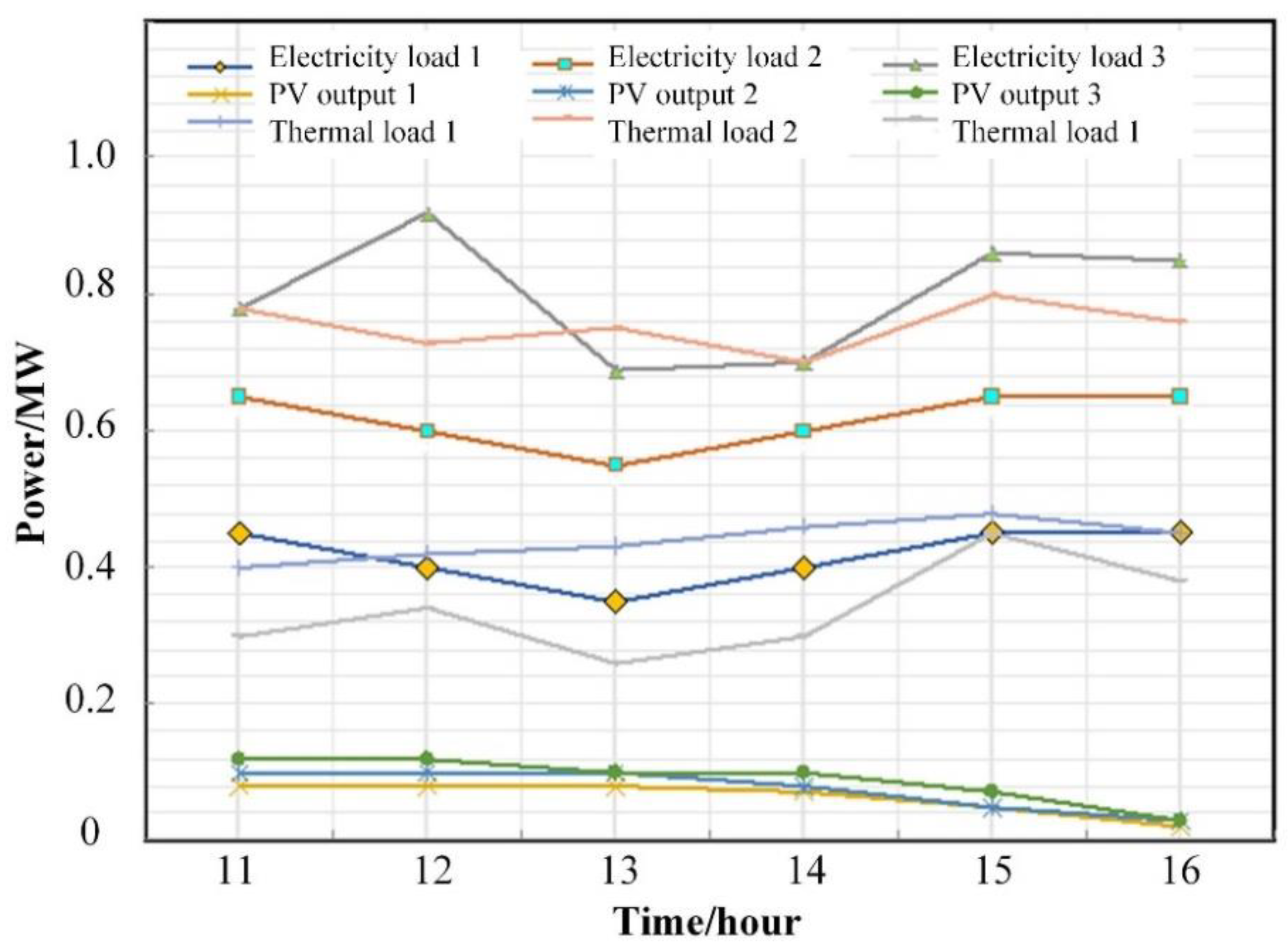
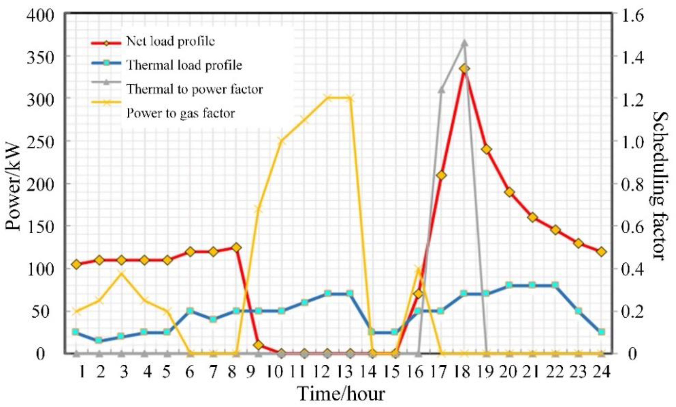
5.2.1. Energy-Consumption Pattern Analysis
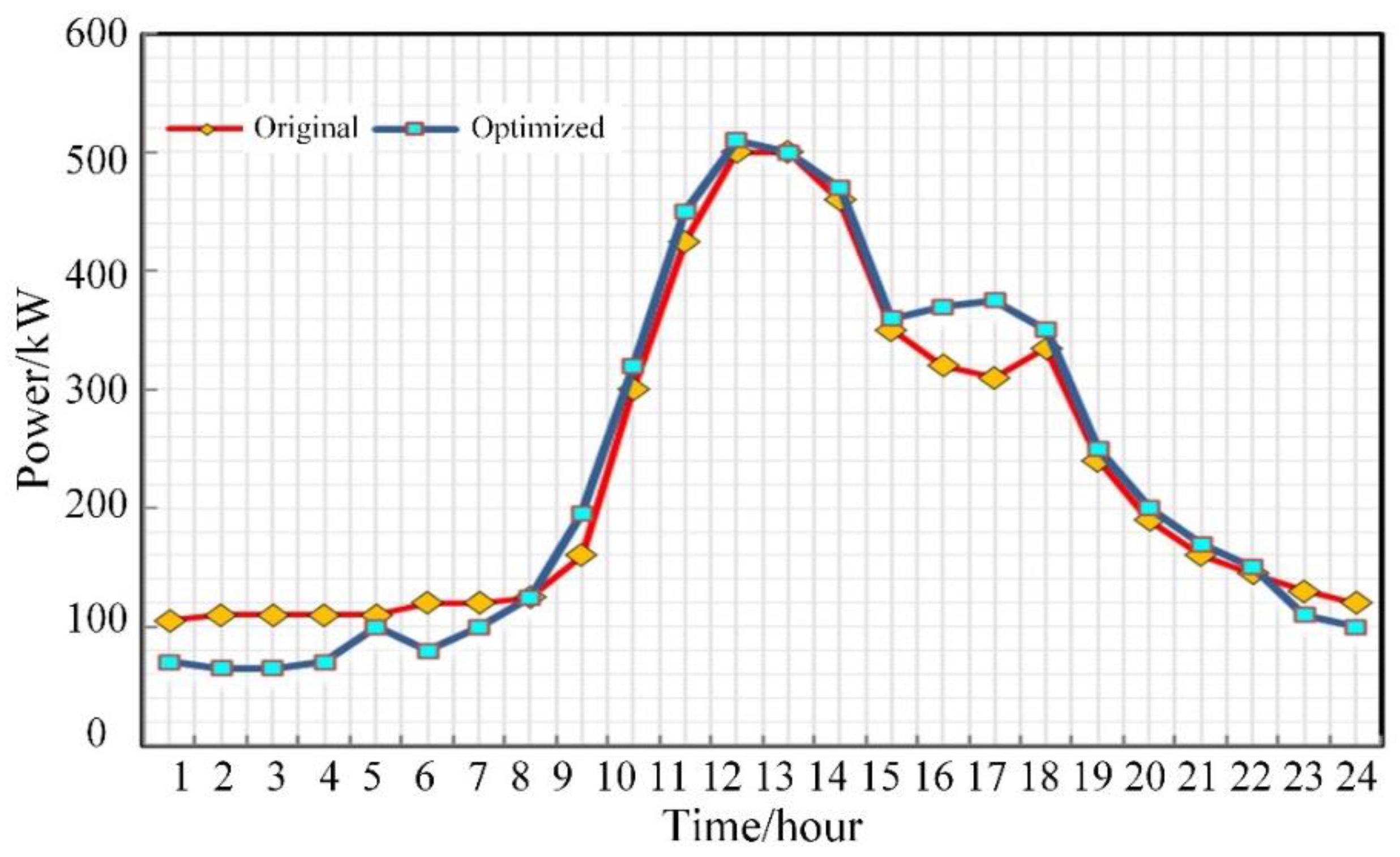
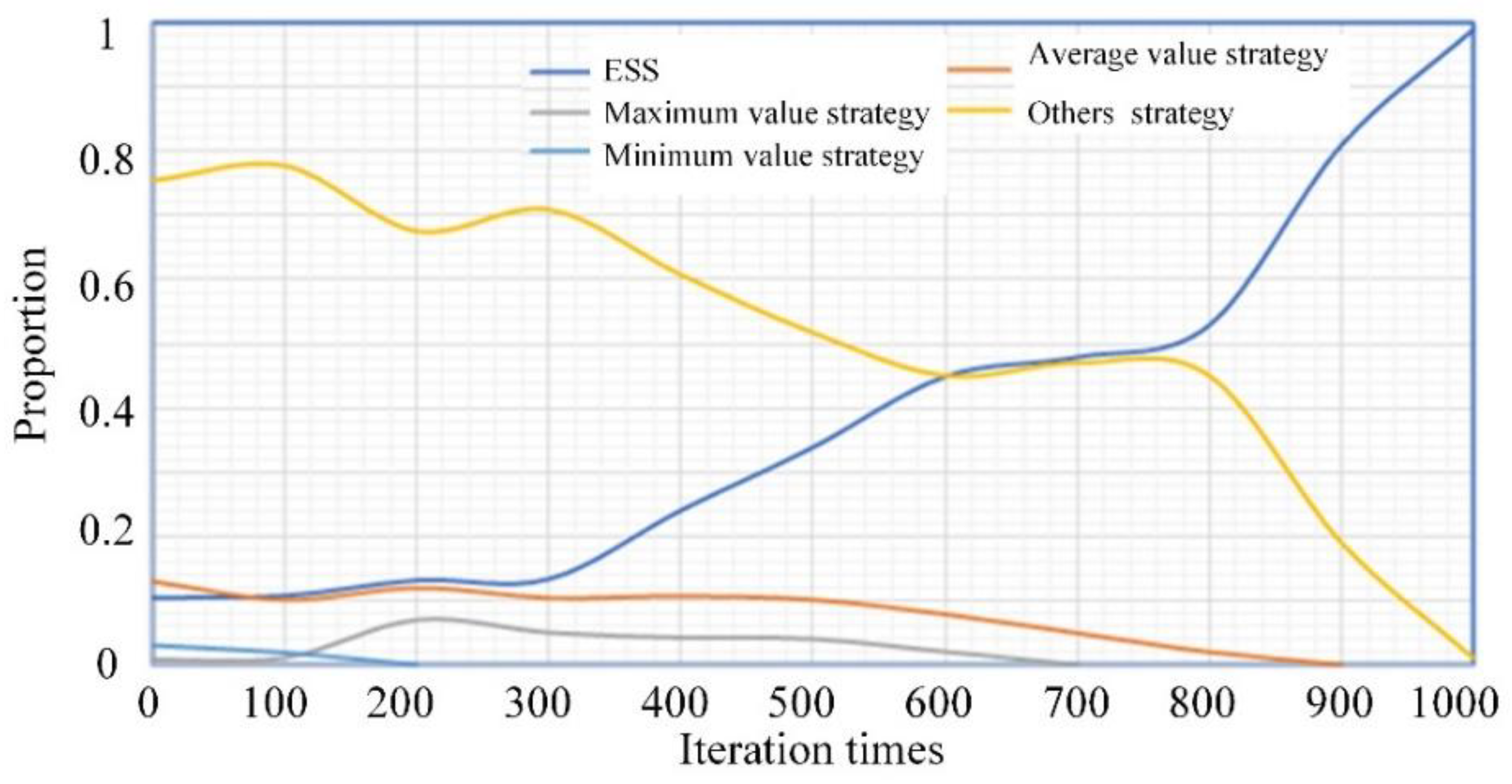
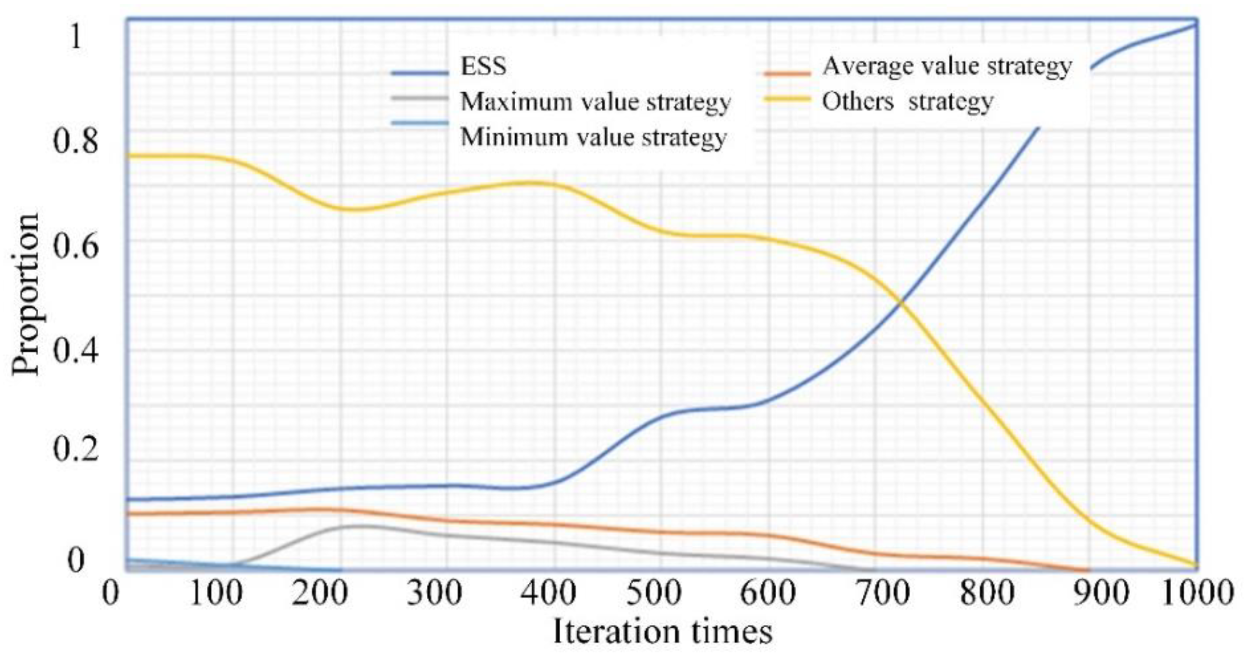
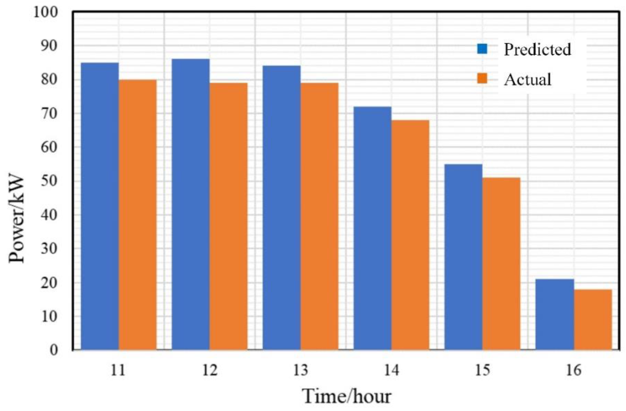
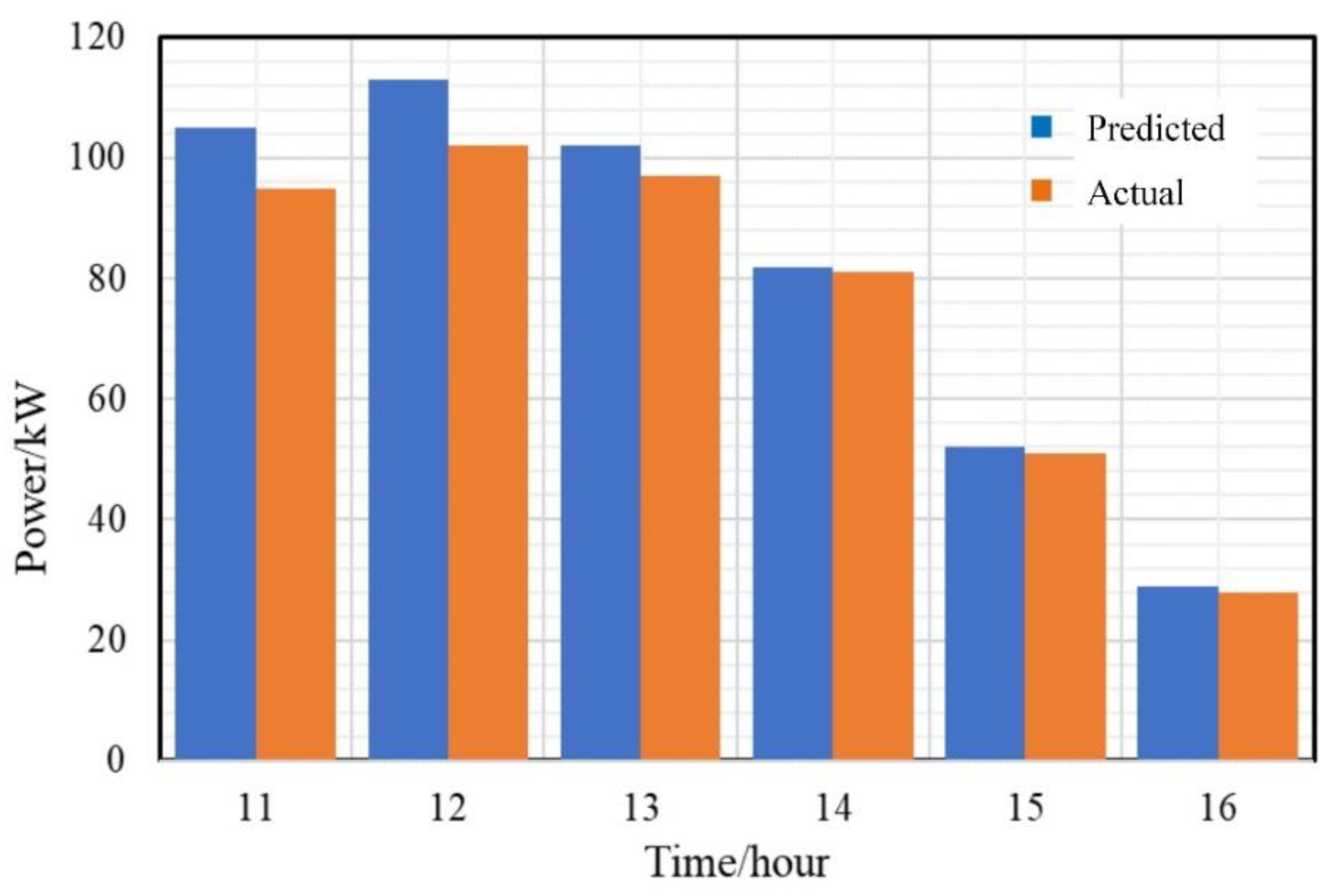
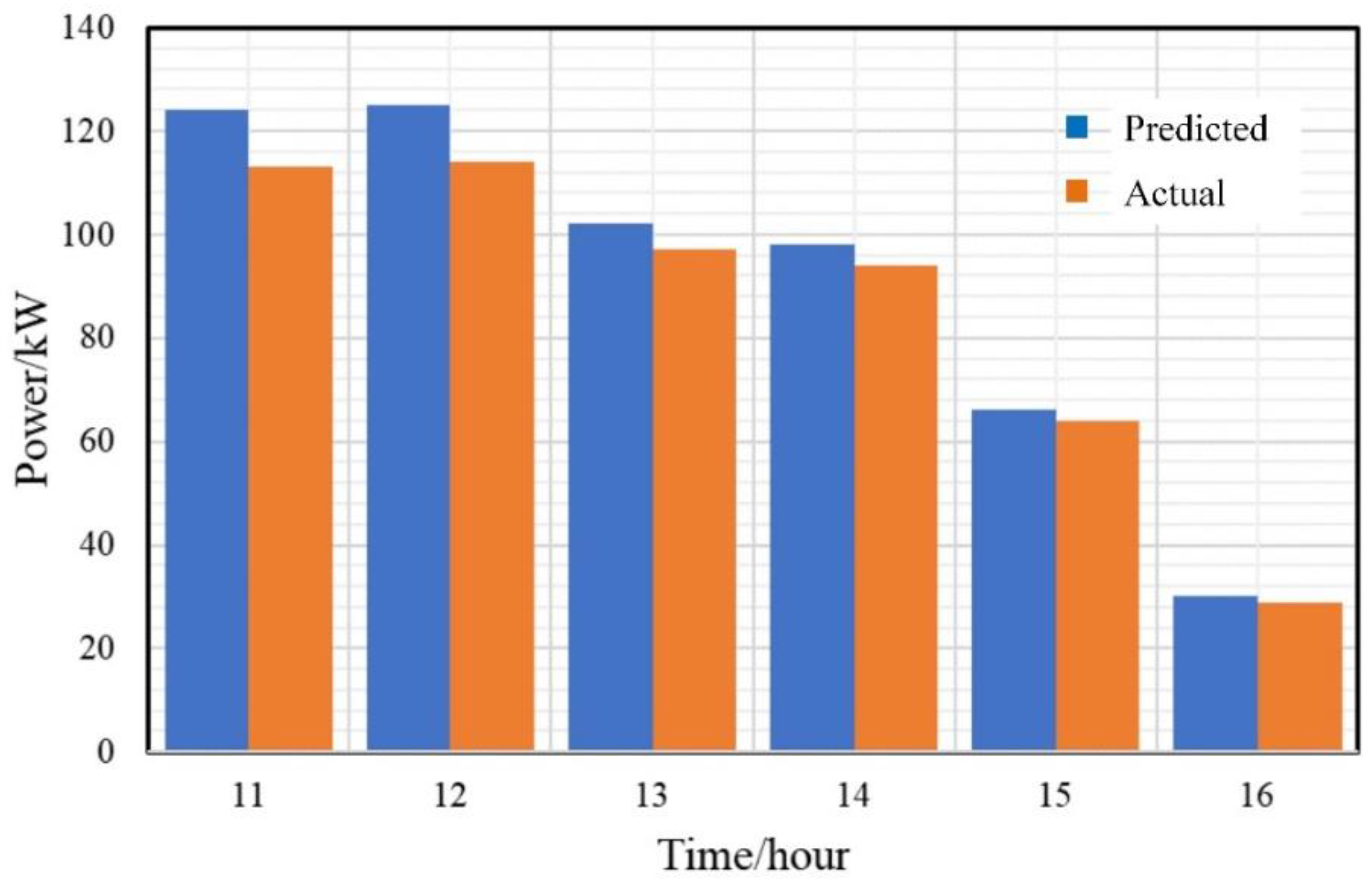
5.2.2. Photovoltaic Output Fluctuation Analysis
6. Conclusions
Author Contributions
Funding
Conflicts of Interest
References
- Li, J.; Liu, J.; Yan, P.; Li, X.; Zhou, G.; Yu, D. Operation optimization of integrated energy system under a renewable energy dominated future scene considering both independence and benefit: A review. Energies 2021, 14, 1103. [Google Scholar] [CrossRef]
- Yousaf, A.; Asif, R.M.; Shakir, M.; Rehman, A.U.; Adrees, M.S. An improved residential electricity load forecasting using a machine-learning-based feature selection approach and a proposed integration strategy. Sustainability 2021, 13, 6199. [Google Scholar] [CrossRef]
- Satymov, R.; Bogdanov, D.; Breyer, C. The Value of Fast Transitioning to a Fully Sustainable Energy System: The Case of Turkmenistan. IEEE Access 2021, 9, 13590–13611. [Google Scholar] [CrossRef]
- Rizwan, R.; Arshad, J.; Almogren, A.; Jaffery, M.H.; Yousaf, A.; Khan, A.; Ur Rehman, A.; Shafiq, M. Implementation of ANN-based embedded hybrid power filter using hil-topology with real-time data visualization through node-RED. Energies 2021, 14, 7127. [Google Scholar] [CrossRef]
- Zeng, A.; Hao, S.; Ning, J.; Xu, Q.; Jiang, L. Research on real-time optimized operation and dispatching strategy for integrated energy system based on error correction. Energies 2020, 13, 2908. [Google Scholar] [CrossRef]
- Li, Z.; Xu, Y.; Fang, S.; Wang, Y.; Zheng, X. Multiobjective Coordinated Energy Dispatch and Voyage Scheduling for a Multienergy Ship Microgrid. IEEE Trans. Ind. Appl. 2020, 56, 989–999. [Google Scholar] [CrossRef]
- Alobaidi, A.H.; Khodayar, M.E.; Shahidehpour, M. Decentralized energy management for unbalanced networked microgrids with uncertainty. IET Gener. Transm. Distrib. 2021, 15, 1922–1938. [Google Scholar] [CrossRef]
- Xu, Y.; Liao, Q.; Liu, D.; Peng, S.; Yang, Z.; Zou, H.; Zhang, L. Multi-player Intraday Optimal Dispatch of Integrated Energy System Based on Integrated Demand Response and Games. Power Syst. Technol. 2019, 43, 2506–2516. [Google Scholar]
- Li, H.; Yu, T.; Qu, K.; Wang, B. Interactive Equilibrium Supply and Demand Model for Electricity-Gas Energy Distribution System with Participation of Integrated Load Aggregators. Autom. Electr. Power Syst. 2019, 43, 32–41. [Google Scholar]
- Liu, W.; Li, X.; Liu, Z.; Wang, K.; Wang, W. Energy operator operating mode and energy management based on Stackelberg game. Mod. Electr. Power 2018, 35, 8–15. [Google Scholar]
- Soliman, H.M.; Leon-Garcia, A. Game-theoretic demand-side management with storage devices for the future smart grid. IEEE Trans. Smart Grid 2014, 5, 1475–1485. [Google Scholar] [CrossRef]
- Chai, B.; Chen, J.; Yang, Z.; Zhang, Y. Demand response management with multiple utility companies: A two-level game approach. IEEE Trans. Smart Grid 2014, 5, 722–731. [Google Scholar] [CrossRef]
- Wu, C.; Gao, B.; Tang, Y.; Wang, Q. Master-slave game based bilateral contract transaction model for generation companies and large consumers. Autom. Electr. Power Syst. 2016, 40, 56–62. [Google Scholar]
- Li, H.; Yu, T.; Zhu, H.; Chen, Y.; Yang, B. Interactive Equilibrium of Electricity-Gas Energy Distribution System and Integrated Load Aggregators Considering Energy Pricings: A Master-Slave Approach. IEEE Access 2020, 8, 70527–70541. [Google Scholar] [CrossRef]
- Gu, J.; Bai, K.; Shi, Y. Optimized Operation of Regional Integrated Energy System Based on Multi-agent Master-slave Game Optimization Interaction Mechanism. Power Syst. Technol. 2019, 43, 3119–3129. [Google Scholar]
- Li, Y.; Wang, C.; Li, G.; Chen, C. Optimal scheduling of integrated demand response-enabled integrated energy systems with uncertain renewable generations: A Stackelberg game approach. Energy Convers. Manag. 2021, 235, 113996. [Google Scholar] [CrossRef]
- Ma, L.; Liu, N.; Zhang, J.; Lei, J.; Zeng, Z.; Liu, W. Optimal operation model of user group with photovoltaic in the mode of automatic demand response. Proc. Chin. Soc. Electr. Eng. 2016, 36, 3422–3432. [Google Scholar]
- Derakhshandeh, S.Y.; Masoum, A.S.; Deilami, S.; Masoum, M.A.S.; Hamedani Golshan, M.E. Coordination of generation scheduling with PEVs charging in industrial microgrids. IEEE Trans. Power Syst. 2013, 28, 3451–3461. [Google Scholar] [CrossRef]
- Ma, Z.; Zhou, X.; Shang, Y.; Sheng, W. Exploring the concept, key technologies and development model of energy internet. Power Syst. Technol. 2015, 39, 3014–3022. [Google Scholar]
- Liu, F.; Pan, Y.; Liu, H.; Ding, Q.; Li, Q.; Wang, Z. Piecewise exponential distribution model of wind power forecasting error. Autom. Electr. Power Syst. 2013, 37, 14–19. [Google Scholar]
- Huo, S. Optimization Method of Source Load Coordinated Operation of Active Distribution Network Considering Source Load Uncertainty; Nanjing University of Posts and Telecommunications: Nanjing, China, 2019. [Google Scholar]
- Zhou, Y.; Yang, M.; Wang, F.; Wang, S.; Zhu, Y. A real-time dispatch model considering the uncertainty in Photovoltaic power. Electr. Power Constr. 2019, 40, 1–8. [Google Scholar]
- Kang, C.; Yao, L. Key scientific issues and theoretical research framework for power systems with high proportion of renewable energy. Autom. Electr. Power Syst. 2017, 41, 2–11. [Google Scholar]
- Jian, X.; You, J.; Liang, Y.; Jia, L. Social influence based close subgraph discovery in social networks. J. Chin. Comput. Syst. 2018, 39, 1342–1348. [Google Scholar]
- Yin, X.; Hu, X.; Chen, Y.; Yuan, X.; Li, B. Signed-PageRank: An efficient influence maximization framework for signed social networks. IEEE Trans. Knowl. Data Eng. 2021, 33, 2208–2222. [Google Scholar] [CrossRef]
- Liu, N.; Chen, Q.; Liu, J.; Lu, X.; Li, P.; Lei, J.; Zhang, J. A heuristic operation strategy for commercial building microgrids containing EVs and PV system. IEEE Trans. Ind. Electron. 2015, 62, 2560–2570. [Google Scholar] [CrossRef]
- Ting, C.; Samdin, S.B.; Tang, M.; Ombao, H. Detecting dynamic community structure in functional brain networks across individuals: A multilayer approach. IEEE Trans. Med. Imaging 2021, 40, 468–480. [Google Scholar] [CrossRef]
- Huang, N.; Bao, J.; Cai, G.; Zhao, S.; Liu, D.; Wang, J.; Wang, P. Multi-agent joint investment microgrid source-storage multi-strategy bounded rational decision evolution game capacity planning. Proc. Chin. Soc. Electr. Eng. 2020, 40, 1212–1225. [Google Scholar]
- Lee, D.; Jeong, J.; Choi, G. Short term prediction of PV power output generation using hierarchical probabilistic model. Energies 2021, 14, 2822. [Google Scholar] [CrossRef]
- Wei, Z.; Liu, L.; Guan, X. Research on Community-Based Energy Internet Operation Considering the Relationship Between Social Networks. Electr. Power Constr. 2019, 40, 36–44. [Google Scholar]


| CIES | CHP Upper Output/kW | PV Capacity/kW | ηe | ηloss | ηh |
|---|---|---|---|---|---|
| CIES1 | 300 | 100 | 0.35 | 0.05 | 0.6 |
| CIES2 | 900 | 200 | 0.40 | 0.6 | |
| CIES3 | 700 | 150 | 0.35 | 0.8 |
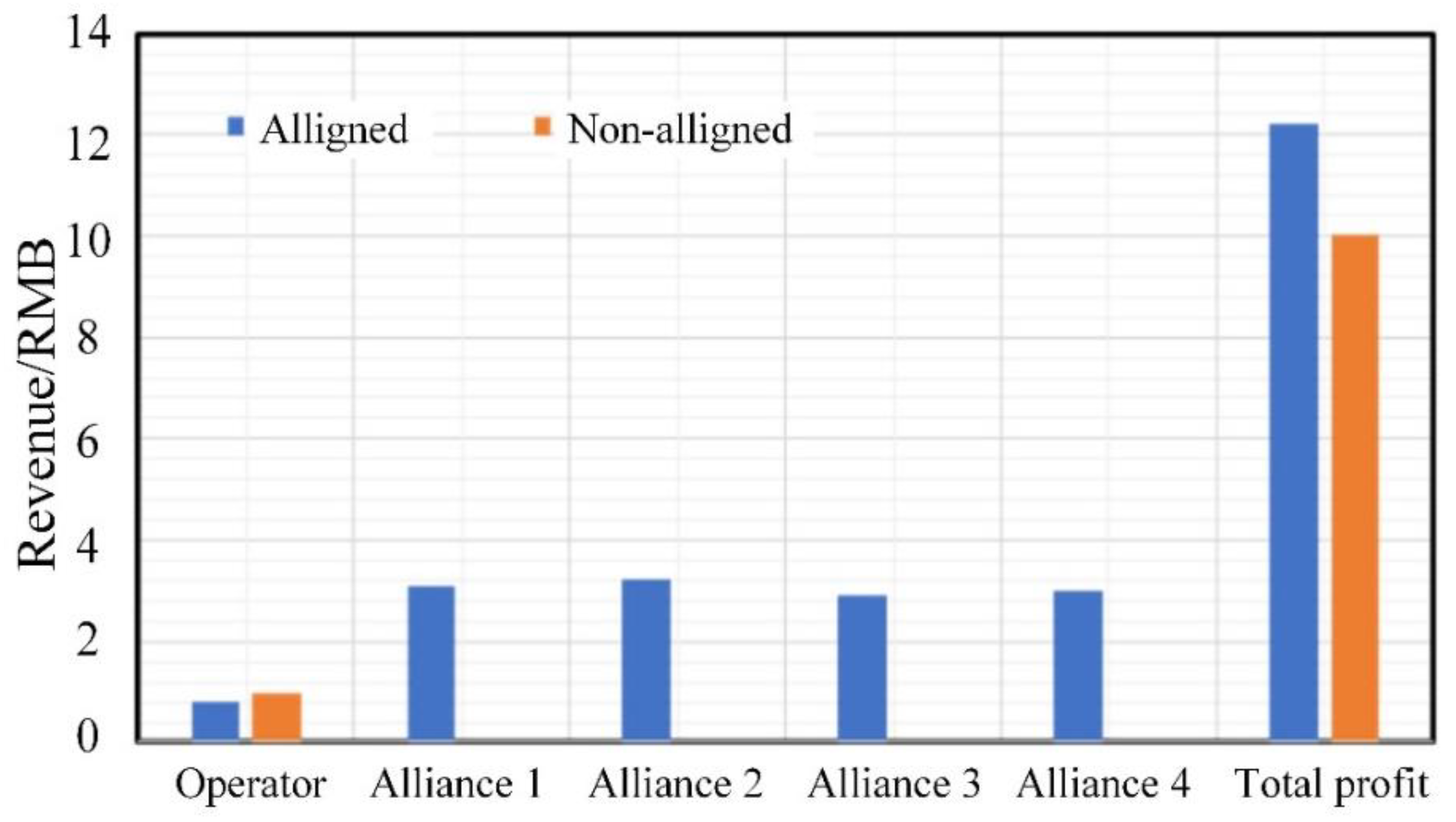
| Number of Alliances | Energy-Consuming Entity Profit (RMB) | CIES Operator Profit (RMB) | RIES Total Profit (RMB) |
|---|---|---|---|
| 2 | 13,732.6 | 683.7 | 14,416.3 |
| 4 | 12,249.8 | 807.5 | 13,057.3 |
| 10 | 11,603.2 | 915.2 | 12,518.4 |
| 20 | 10,316.1 | 1004.5 | 11,320.6 |
Publisher’s Note: MDPI stays neutral with regard to jurisdictional claims in published maps and institutional affiliations. |
© 2022 by the authors. Licensee MDPI, Basel, Switzerland. This article is an open access article distributed under the terms and conditions of the Creative Commons Attribution (CC BY) license (https://creativecommons.org/licenses/by/4.0/).
Share and Cite
Li, W.; Tang, M.; Zhang, X.; Gao, D.; Wang, J. Optimal Operation for Regional IES Considering the Demand- and Supply-Side Characteristics. Energies 2022, 15, 1594. https://doi.org/10.3390/en15041594
Li W, Tang M, Zhang X, Gao D, Wang J. Optimal Operation for Regional IES Considering the Demand- and Supply-Side Characteristics. Energies. 2022; 15(4):1594. https://doi.org/10.3390/en15041594
Chicago/Turabian StyleLi, Wenying, Ming Tang, Xinzhen Zhang, Danhui Gao, and Jian Wang. 2022. "Optimal Operation for Regional IES Considering the Demand- and Supply-Side Characteristics" Energies 15, no. 4: 1594. https://doi.org/10.3390/en15041594