The Impact of Detail, Shadowing and Thermal Zoning Levels on Urban Building Energy Modelling (UBEM) on a District Scale ^†

Abstract

New modelling tools are required to accelerate the decarbonisation of the building sector. Urban building energy modelling (UBEM) has recently emerged as an attractive paradigm for analysing building energy performance at district and urban scales. The balance between the fidelity and accuracy of created UBEMs is known to be the cornerstone of the model’s applicability. This study aimed to analyse the impact of traditionally implicit modeller choices that can greatly affect the overall UBEM performance, namely, (1) the level of detail (LoD) of the buildings’ geometry; (2) thermal zoning; and (3) the surrounding shadowing environment. The analysis was conducted for two urban areas in Stockholm (Sweden) using MUBES—the newly developed UBEM. It is a bottom-up physics-based open-source tool based on Python and EnergyPlus, allowing for calibration and co-simulation. At the building scale, significant impact was detected for all three factors. At the district scale, smaller effects (<2%) were observed for the level of detail and thermal zoning. However, up to 10% difference may be due to the surrounding shadowing environment, so it is recommended that this is considered when using UBEMs even for district scale analyses. Hence, assumptions embedded in UBEMs and the scale of analysis make a difference.

1. Introduction

Buildings are responsible for one-third of the total final energy use and nearly 40% of total greenhouse gas emissions [1]. Hence, this sector is one of the key contributors to climate change and should be addressed in order to meet the 1.5 °C scenario [2]. There is a wide range of mitigation options available including the decarbonisation of supply, refurbishment of the existing building stock, and near-zero energy requirements of new buildings. However, the current speed of building energy transition is much slower than what is needed to meet national and local climate commitments [3]. New decision-making paradigms and tools are required to improve the overall efficiency of the building sector. There is an urgent need for integrated models and tools that would allow for the assessment of the benefits and deficiencies of each urban energy intervention in a holistic manner for all of involved stakeholders.

The initial uptake of city-scale building energy modelling was captured in the reviews by Swan and Ugursal [4] and Kavgic [5], which provided categorisation of the models into top–down and bottom–up, where the latter were divided into statistical and engineering. Top–down approach imposes the representation of the entire building stock as a single unit of analysis. In contrast, the bottom–up approach intends to focus on individual buildings. In their turn, statistical and engineering stand for data-driven or physics-based models being later joined by hybrid reduced-order models combining both approaches. The subsequent review by Reinhart and Davila [6] introduced the term of ‘Urban Building Energy Modelling (UBEM)”, which was attributed explicitly to bottom–up engineering models. This approach is different from a plain assembly of single building energy models (BEM) as it creates the automated generation of simulations based on larger amounts of structured data and a more simplistic representation of individual buildings. Most of the recent review papers have tended to focus on these types of models such as UBEMs, systematising their functional components [7], applied approaches [8], and key challenges [9]. However, a recent review by Ali et al. [10] returned to a wider scope, providing a comparative analysis of modern top–down and bottom–up urban-scale energy models.

A number of UBEM environments and tools have been developed in recent decades [11]. These include UBEMs using more detailed physics-based thermal engines such as EnergyPlus (CityBES [12], UMI [13]), simpler reduced-order models based on self-made RC networks (DIMOSIM [14], CitySim [15] or not formally named [16]), energy signatures [17], or the ISO/CEN standard method (SimStadt [18], CEA [19]). The review of UBEM cases in [20] shows that the choice of the model can be attributed to the project constraints, data and skills’ availability, and, ultimately, the purpose of developed UBEM. The issue of scale has been addressed in different ways [7] including various approaches to align the created urban scale models with measured data using probabilistic calibration [21,22]. In the UBEM field, physics-based multizone dynamic models are required to evaluate design scenarios for new urban areas or carbon reduction strategies to existing building stock such as urban scale building retrofitting [6]. However, in the case of large scales, even a slight increase in resolution for one or more aspects of UBEM (e.g., spatial, temporal, scenario space) can lead to a noticeable growth in the computational burden due to the issue of dimensionality. For instance, more detailed thermal zoning will require that the higher system’s dimensions are solved. In addition, another serious bottleneck for introducing higher spatial resolution to UBEM is traditionally the limited data availability.

The balance between model fidelity and accuracy is a key issue in UBEMs. Many studies have utilised archetypes (representative buildings for a group of similar buildings) to lower the number of simulations needed on a city scale [17,23,24]. A number of studies have investigated the impact of choices made when a new UBEM is set up. Three fidelity-related aspects have been regularly highlighted as having a crucial impact on the quality and applicability of the derived UBEMs, namely (a) the level of detail (LoD) of buildings’ geometry [25], (b) thermal zoning [26], and (c) the shadowing effect of the surrounding environment [27]. Hence, the main value of the proposed study is in characterising the impact of these implicit assumptions on the quality of UBEMs. This contribution is expected to raise the awareness of scholars and practitioners, provide more ground-based reasons in making these modelling choices, and finally, improve the quality of decision-making based on these promising and powerful modelling tools.

This paper aimed to investigate the impact of the typical choices made at the UBEM generation stage, namely around the level of detail (LoD) of building geometries, the approach to thermal zoning, and the boundaries of the surrounding environment to be considered for shadowing. The study utilised MUBES (Massive Urban Building Energy Simulations)—a novel UBEM simulation tool presented in Section 2. The two urban districts, Minneberg and Hammarby Sjöstad (Stockholm, Sweden), used for the case study are described in Section 3. The analysis of the impact of LoD, thermal zoning, and shadowing is provided in Section 4. Finally, Section 5 summarises the paper with a discussion and our conclusions.

2. MUBES—An Open Tool for Urban Building Energy Modelling (UBEM)

2.1. UBEM Workflow

This section describes the methodology of MUBES—the new generation UBEM used for the analysis in this study. MUBES is a bottom–up physical UBEM providing a common framework for the computation of an individual buildings’ energy demands in urban areas by using the data from various public data sources as inputs for dynamic building physics models. These building energy models follow a shoebox paradigm and are automatically generated for each individual building. These are composed of two levels: the building and the zone levels.

The building level requires building geometry with its surrounding environment, internal thermally conditioned zones/volumes delimitation, and some elements that characterize the performance of the building’s envelope. The related inputs are assumed as static ones for the UBEM workflow as these are not time dependent on a yearly time basis. The zone level requires indoor elements and occupancy related inputs that have time-related impacts on energy needs. Hence, along the UBEM workflow, the latter inputs can be seen as dynamic ones. Internal heating and cooling production equipment are situated at the zone level as different production types can be present in the same building. Following the same paradigm, envelope leaks with time dependent impacts (from variables such as wind, pressure, and temperature) are also situated at the zone level. These can be differently addressed, depending on the type of zone (heated or non-heated).

The overall workflow can be described with four main steps (Figure 1): (I) data integration; (II) the generation of building models; (III) run of building energy simulations; and (IV) output and aggregation of results.

The UBEM can be used in either building per building or archetype-based simulation modes. In both cases, a physics-based white box model was defined with as many elements as possible. The current version of UBEM was based on Python 3 for the structuring process and EnergyPlus 9.1 for the thermal core engine. Multithread processing was implemented for the computationally intensive processes (the generation of models and dynamic thermal simulations). While the basic function uses the eppy python package [28], a special branch was created using the geomeppy package [29] in order to enhance the thermal zoning method and enable complex building footprints to be considered. The tool with sample data is freely available under MIT license at https://github.com/KTH-UrbanT/mubes-ubem (accessed on 19 January 2022). The following subsections present the details of the used UBEM workflow for (I) data integration (Section 2.2); (II) generation of models on building (Section 2.3) and zone (Section 2.4) levels; (III) simulation options (Section 2.5); and (IV) results output (Section 2.6).

2.2. Data Integration

The process of data integration followed the Extract, Transform, Load (ETL) paradigm implemented in the Feature Manipulation Engine (FME) from SAFE software as described in [30]. The initial data sources and subsequently generated data inputs provided to MUBES UBEM are depicted in Figure 2.

All building information was blended in FME to generate two GeoJSON files for each urban area analysed. GeoJSON is a standard geospatial data interchange format chosen due to its universality and human readability. The first file, Buildings.geojson contained a set of geometric (MultiPolygon) and non-geometric features, where the latter could include all attributes from the linked records for property and building cadastres (such as building purpose or form of ownership) and the energy performance certificate (EPCs) database. The second file, Walls.geojson, contained the geometric features (Linestrings with a range of heights) representing the shadowing environment for the whole district. Each building listed in Buildings.geojson was provided with a list of walls affecting the sun exposure of a particular building using the identifiers from Walls.geojson. This second file (Walls.geojson) was only needed to model the shadowing effect of the surrounding environment. In the case of larger urban areas, up to the city scale, several GeoJSON file pairs are generated.

EPCs are the essential data source in this UBEM workflow. Despite this policy instrument being universally adopted across the whole of the EU, its implementation and the quality of the resulting datasets can differ among EU member states [31]. In Sweden, EPCs are produced by independent energy experts and collected by the National Board of Housing, Building, and Planning (Boverket). EPCs are required for all larger buildings every 10 years and are based on the yearly data of the energy consumption split by different needs (space heating and cooling, domestic hot water, electricity, subdivided into collective and private areas) and energy carriers. The data origin can either be from energy supplier invoices or measured using devices especially designed for EPCs. The numeric values can be obtained either from installed meters or from the yearly collection of invoices from energy suppliers. Data gathered in EPCs also includes some useful details on the building geometry, installed equipment, occupancy type, etc.

Swedish EPCs possess a reasonable quality of data that allows them to be widely used for analysis on an urban scale [17,32]. However, they are also prone to certain problems. For instance, the time lag imposed by the methodology of the EPC data collection can result in missing effects from recent building retrofitting (be it either envelope or equipment), leading to model performance gaps. As was shown previously in [31,33], heated area attributes (area heated above 10 °C) are the key source of uncertainties in EPCs and models utilising this data source. Therefore, at the transformation stage, data from EPCs were cross-validated and enriched from other sources including building and property cadastres from Lantmäteriet and point cloud building data from the Stockholm municipality.

The following subsections describe the process for generating the energy model based on the input data provided in the main GeoJSON file.

2.3. Generation of Models—Building Level

This level is about geometry definition, thermal zoning, surrounding environment, and envelope characteristics. Each are presented separately in the following subsections.

2.3.1. Geometry Definition

Building footprints from the Swedish property map (2D) were used as the basis for the 3D model. The polygons were integrated with the EPC register by using an ETL method developed by [30,32] to obtain additional information, which was later used by the simulation engine. Each building footprint was used to clip a photogrammetric point cloud and a terrain model, which was used to calculate the median roof height and ground height of the building. 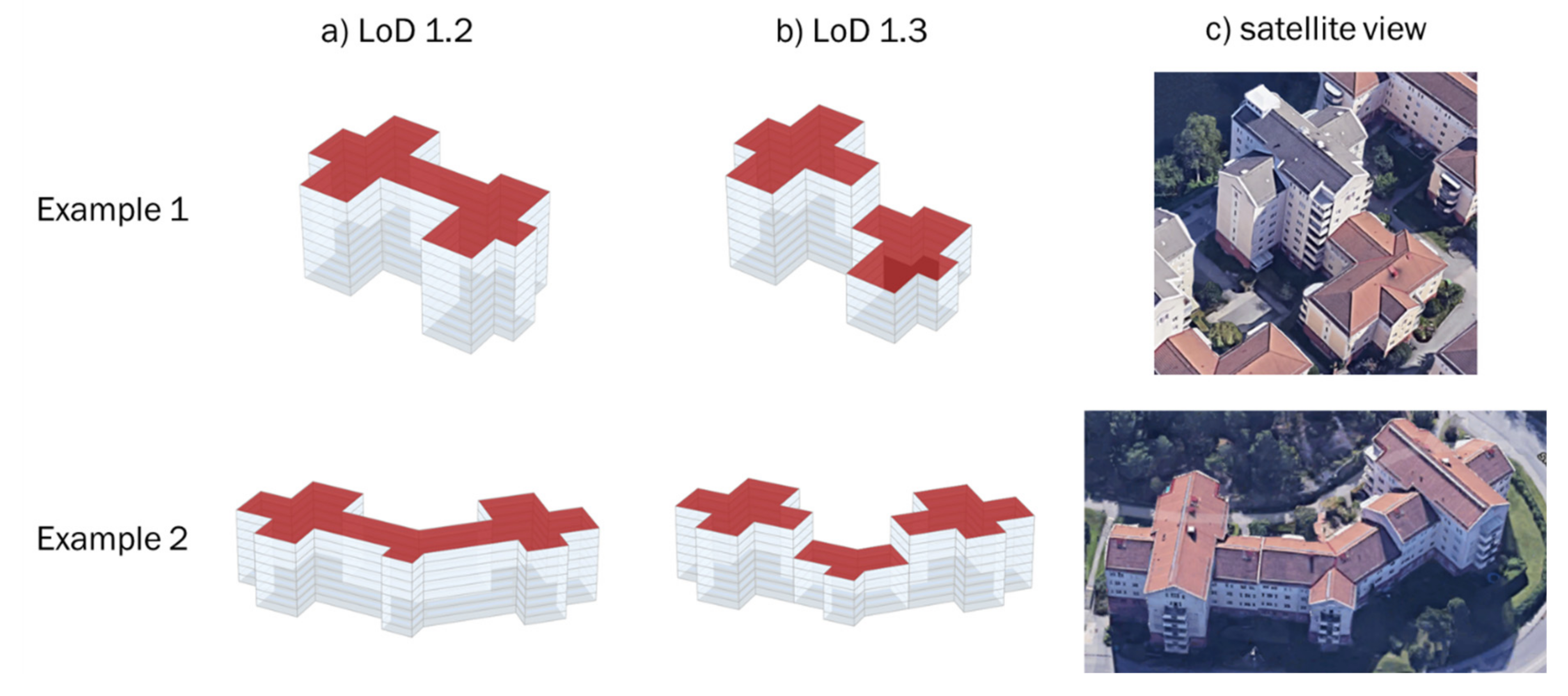This method is described further by [30,32] and was designed either to make LoD 1.2 or 1.3, considering the classification proposed in [25]. Being based on CityGML 2.0 specification ranging from LoD 0 (footprint) to LoD 4 (contains indoor features), it provides a more fine-grained specification of LoDs, specified by four sublevels for each LoD 0–3.

Building footprints from the property map can (in general) can only be used to create LoD 1.2, which can create a high deviation in building volume compared to the actual building. This is especially the case for buildings that consist of a large variety of building heights. The volume deviation can be decreased by creating LoD 1.3. This LoD does not result in a high increase in the number of surfaces compared with more detailed LoD levels [25], which is important for UBEM, as an increase in the number of surfaces for each building results in more intensive energy calculations.

To test the impact of using LoD 1.3, a method of segmentation of building footprints by different roof heights was developed. The point cloud was first cleaned by filtering 5% of the highest and lowest points and triangulating the remaining points. Triangles with high vertical slopes were kept and dissolved with their neighbours and later replaced with a centreline. Snapping was used to extend the centreline to the correct boundaries of the building footprint. The centreline was then used to cut building footprints in several parts. The median and ground height were then recalculated. Each building footprint and building part was generalised using the Douglas algorithm to minimise the number of vertices, and segment snapping was applied to remove small distances between footprints. To create the 3D model, the building footprint was set at the median ground height and was then extruded to the median roof height.

The 3D model was also used as an input to create a neighbourhood shading walls file to supply the simulation engine for shadowing computations. The buildings in the 3D model were de-aggregated into 2D lines with ground height and roof height stored as two attributes, creating a light dataset that would also be possible to re-generate later in the simulation engine. All lines were replaced by a centre point that was used to find all neighbouring points within a 250-m radius. All points were connected by a line to represent the line of sight; lines that crossed one or more buildings were filtered out. For each building, a list of the remaining walls was stored, and duplicates were removed. Finally, the walls file was created with a unique id of the walls with a corresponding wall id in the 3D buildings file. This made it possible to obtain fast and accurate neighbouring walls for a building. A low calculation time was achieved as the calculation was conducted entirely in 2D, and the height of the building and terrain was not considered, which may lead to less accurate energy calculations for some buildings.

In Section 4, the impact of the above-mentioned level of details from LoD 1.2 to LoD 1.3 is quantified for one specific district.

2.3.2. Envelope Characteristics

Since fewer elements are available for analysis at the urban scale, the envelope characteristics are in two different layers, representing the insulation effect and the inertia effect, respectively. This differentiation allows for the modelling of either lightweight or heavyweight buildings as being well insulated or not. The position of both layers can also be defined in order to capture the impact of external or internal insulation on the envelope. The definition of these lumped layers follows the resistance/capacitance paradigm for layers in a series as 1D conduction was considered in the thermal engine. Three main thermal properties are required for the layers composed of one single material, other than the thickness, namely: density (kg/m³); thermal conductivity (W/K/m²); and specific heat capacity (J/K/kg). Specific surface properties such as radiative properties can be defined at this stage if a specific effect is to be considered (e.g., special paint coatings or metallic surface layers). Windows are part of the envelope. The window to wall ratio (WWR) is defined as an input. Window width overlaps 95% of the zone width and the height is computed using the input given for WWR. Their energy performances are also defined in the input data.

2.3.3. Thermal Zoning

Several options for thermal zoning are implemented, from the single zone for heated and non-heated volumes up to the core and perimeter zoning option on each floor. In the case of aggregation of different floors into a single zone, the inputs are still represented at the floor level, but are then further corrected using a floor-multiplier factor, as proposed in [26]. The core and perimeter zoning option required a specific algorithm. Depending on the perimeter depth, the perimeter zone definition is automatically created starting from each edge, delimiting the core zone. The core zone definition includes a threshold for the resulting vertex’s distance within three vertexes. This threshold is, by default, set to a half of the perimeter depth. This allows us to avoid having too narrow zone angles, too small edges, or too small zones. Then, for the perimeter zones, triangle zones (having a single vertex on the external polygon) are not allowed, except for the last perimeter zone definition, closing the loop over the edges of the core. Thus, perimeter zones with more than one edge in common with the core zone are allowed. The perimeter depth starts at 3 m by default and is reduced by half if any issue is encountered during the process. This algorithm was derived from the original one given in the Geomeppy package [29]. Figure 3 presents the thermal zoning options and the effect of the perimeter depth for two sample buildings.

As shown in Figure 3, non-convex zones are currently allowed, thus all external non-convex surfaces were split further into convex ones for the purpose of shortwave multireflection (see Surrounding Environment Section 2.3.4). Internal non-convex surfaces were not treated further. Internal convex ones are only needed if internal shortwave multireflection is required, which is not of concern in the case of UBEM, as no internal architecture would be available at this scale of analysis.

2.3.4. Surrounding Environment

The shadowing impact from the surrounding environment was considered for each building. Shadowing is automatically dealt with in EnergyPlus by using the shadowing element object. External surfaces can still receive and reflect shortwave radiation, but longwave radiation exchanges are not considered. The latter would have required the computation of the view factors between each surface before simulation, and then the use of an iterative approach to capture the heat fluxes between surfaces at each time step. Some proposals for iterative methods have been suggested by [34]. The maximum effect of a 3.6% decrease in heat needs have been observed in different locations in the U.S. In the proposed UBEM workflow, all external surfaces are sequentially considered for each building, and all visible surfaces belonging to other buildings (included in the Walls.geojson file introduced earlier) are reported. Then, depending on a threshold for the distance from the building’s centroid, surfaces beneath the limit are viewed as shadowing surfaces in EnergyPlus. Figure 4 illustrates the distance threshold on the modelling process for one random building.

Parametric simulations for two different districts are reported in the Results (Section 4).

2.4. Generation of Models—Zone Level

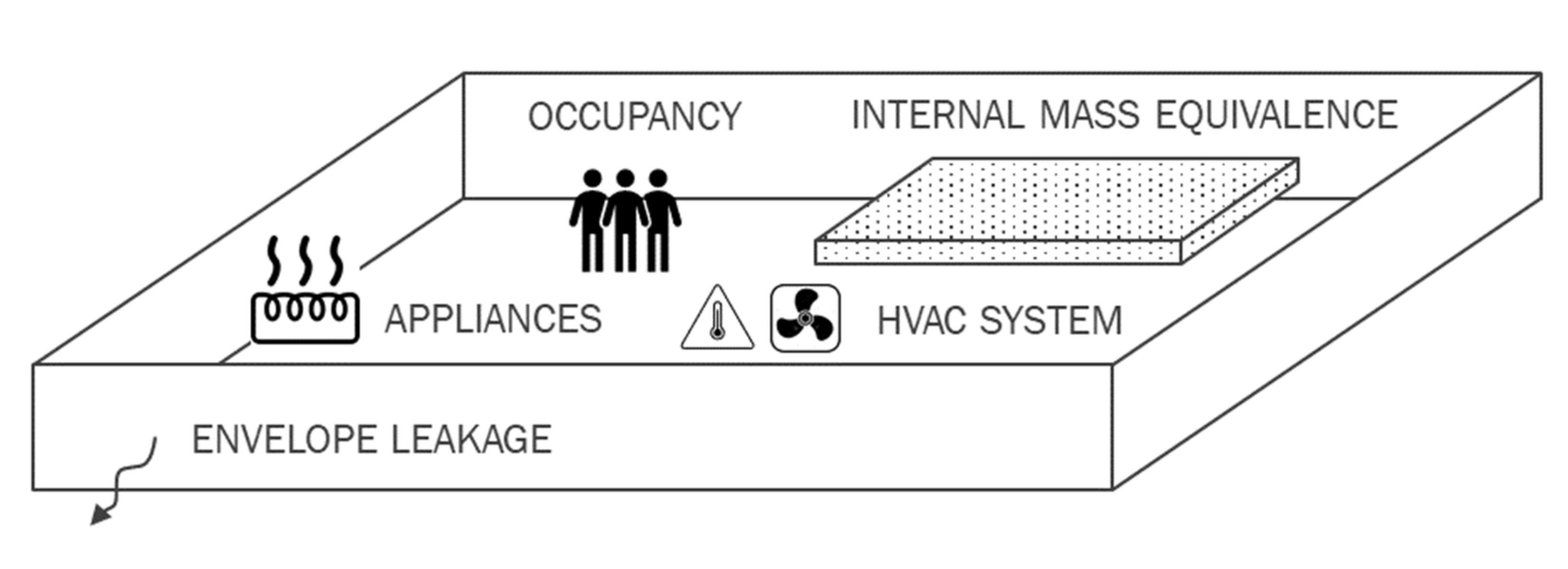
This level concerns all local elements that have a time dependent impact on the zone’s energy balance. Figure 5 represents the different required inputs for this level. All are presented in the following subsections.

2.4.1. Internal Mass Equivalence

The buffering effect on indoor temperature dynamics from internal furniture and partition walls is modelled through an internal mass object. The buffering effect is of greater importance in UBEM assumptions as the internal architecture is unknown. Indeed, all zones are defined as open spaces in which area-based elements are given as inputs. Internal mass object is equivalent to a material with classic thermal properties with an amount defined by weight per square meter and a link with the zone’s ambient air through a surface of exchange. In the proposed UBEM, the default values are 40 kg/m² of an equivalent material with the following properties: thermal conductivity of 0.3 W/K/m, density of 600 kg/m³, and specific heat of 1400 J/kg/K. The surface of exchange is twice the floor area as in [35]. The floor-multiplier is also used when thermal zoning is considered (single zones for heated and non-heated volumes).

2.4.2. Envelope Leakage

Envelope leakage is of great importance. It is influenced by the thermal gradient between indoor and outdoor conditions and the zone’s height (used to compute the hydrostatic pressure gradient). Several other elements can influence related heat transfer such as stairwells, urban area density, and the building’s height. The EnergyPlus infiltration model with flow coefficient enables us to consider these influenceable factors. In the proposed UBEM, a value of 0.667 was used for the pressure exponent value in the power law. In Sweden, the above listed influenceable parameters are given in the EPC’s templates.

For non-heated zones, instead of the above-mentioned model, an air change rate is defined in hours per volume. This approach makes more sense for use with below ground levels without using pressure balance solvers.

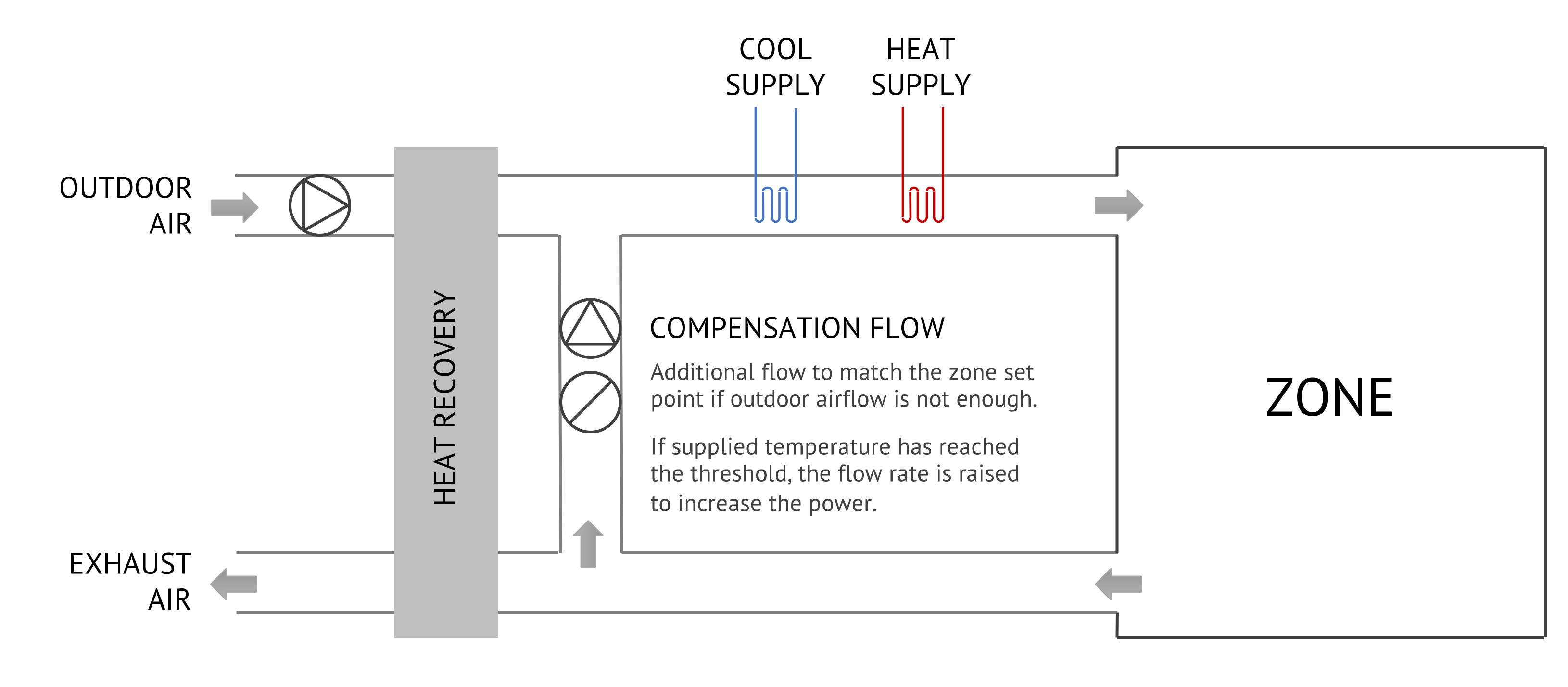
2.4.3. HVAC System

In the proposed UBEM workflow, the focus is on the used-energy needs. This means that the energy carriers as well as their production and distribution efficiencies are not considered at the zone level, but are accounted for in the post-treatment and calibration stages, as will be further described. The heating, ventilation and air conditioning (HVAC) system shall thus be able to represent any kind of system embedding the indoor renewable air change rate including any potential heat recovery from it. An equivalent shoebox HVAC model was considered with the Ideal Loads Air System object, which computes, for each zone, the needed energy to match the internal temperature set point. Figure 6 presents a schematic view of such a system. A limitation can be specified for either the supplied air temperature or compensation mass flow rates of the overall supplied power. The heating and cooling supplies will, at each time step, correspond to the external needed energy for this zone to comply with its temperature setpoint. The temperature setpoint can be defined as either constant or from fixed schedules for day and night times, or even through an external file. In the proposed UBEM workflow, each zone has its own HVAC system.

2.4.4. Occupancy

Occupancy rate can have a strong impact on the energy balance in non-residential types of buildings. In contrast to residential buildings, the number of occupants steers the air change rate and can cause significant heating effects (considering each occupant releases an average of 70 W, 15 people produce more than 1 kW of heating). The occupation density is lowest, by a large margin, in residential type buildings and does not affect the ventilation rates (the occupant’s activity can if the system is demand-controlled based). Thus, for the latter type of buildings, the impact of occupancy can be embedded in the appliance’s energy needs. In the proposed UBEM workflow, two options are available using either the maximum density per type of activity or hourly numbers of occupants based on random beta distribution. Scheduled timetables have also been proposed using opening and closing hours.

2.4.5. Appliances

The energy used and released by internal appliances is considered through lumped values to further decline into hourly data. Thus, a higher time resolution than just the yearly values of W/m² are required. Starting from a yearly value given in EPCs or other databases, the cumulative distribution of internal gain is represented by a reversed sigmoid. Equation (1) represents the cumulative distribution of internal load (CDIL) function in a regular sigmoid shape. The seasonal effect can be tuned by the slope factor $\gamma$, which would represent a greater seasonal effect for greater values. The regular sigmoid curve would represent more internal gains during the summer period (considering a starting period of the first of January), while a 6-month offset should be introduced to represent more internal gains during the winter period. A 6-month offset was thus introduced and normalised CDIL computed. Figure 7 presents the slope factor effect on the normalised CDIL. The derivative values of the CDIL were written in an external file defined as an input file of hourly watts per square meter in EnergyPlus using the electric equipment object in each heated zone.

$$CDIL=\frac{YearlyConsumption}{\left(1+exp\left(-\gamma t\right)\right)}$$

(1)

2.5. Simulation Options

2.5.1. Domestic Hot Water

The proposed UBEM workflow assumes that domestic hot water (DHW) does not contribute to providing heat to the building. The option of modelling DHW would thus be steered by the calibration stage, using aggregated measured data for both space heating and DHW. In such cases, the related energy needs for DHW are modelled through a simple water use equipment object. The temperature of the hot water supply was fixed at 55 °C by default, and the temperature of hot water from the water tap was fixed at 37 °C by default, and the temperature of the cold-water supply was defined through the time series’ input (or taken as constant). Together with water tap usage patterns, this results in the energy needs for DHW. As DHW might only be considered for the calibration stage (Section 2.5.2), the FMI option (Section 2.5.3) could be used to compute the water tap usage to diminish the discrepancies between the measured and simulated energy needs in non-heating periods.

2.5.2. Calibration

Despite UBEM not being a simple aggregation of BEMs, a calibration process for accurate models is still required. Even though a number of simplifications have been made in UBEMs when compared to BEMs, many inputs are still needed, which are usually associated with higher uncertainties than single BEMs. The UBEM calibration process needs to be adapted for each type of building. Hence, while missing inputs can be more or less the same for a whole sample of buildings, the calibrated inputs would definitely be different.

The probabilistic calibration has been repeatedly reported as the best fit for UBEM applications [21,22]. The iterative Bayesian process has been found to be particularly promising as it allows for the automatic adjustment of the exploring ranges for missing inputs for each building. The developed UBEM workflow is fully compatible with this technique. It provides the option of conducting numerous simulations with Latin Hypercube Sampling (LHS) for any input parameter(s) for the purpose of either sensitivity analysis or model calibration.

2.5.3. Co-Simulation Environment

The co-simulation option implemented in MUBES follows the paradigm of a functional mock-up interface (FMI) [36]. Functional mock-up units (FMU) are to be built for any model (building) that may need adjustment of one or more inputs or parameters during the simulation. All the FMUs were used in an environment dedicated to running FMUs. The FMU toolkit for EnergyPlus [37] is embedded in the MUBES UBEM workflow. FMUs can thus be automatically generated for each building in the input file. This requires the definition of specific inputs and outputs to be matched with the controlled parameters targeted in co-simulation. For the proposed UBEM tool, two examples of co-simulation are proposed using the indoor temperature setpoint and the DHW tap usage as inputs at each time step.

2.6. Output of Results

All variables available from EnergyPlus can be given as the output in the UBEM workflow. As post-treatment might be specific to each case studied, some generic methods are proposed in the UBEM, but only for the sake of illustration.

In the following sections, the above described UBEM workflow was used to make parametric simulations. The impact of the level of detail (LoD) is first highlighted, followed by thermal zoning, and the shadowing of the surrounding environment. Two different districts in Stockholm County are used for illustration. After an initial presentation of the two districts and the related database construction process, the results are presented.

3. Case Study

Two districts in Stockholm (Sweden), Minneberg and part of Hammarby Sjöstad, were considered for the impact analysis using parametric simulations (Section 4). Both districts are mainly residential, however, most of the analysed buildings include a small percentage of non-residential occupancy. Minneberg, and the analysed part of Hammarby Sjöstad, are composed of 33 and 45 buildings, respectively (Figure 8). Minneberg was developed in 1987 and is distinctive for the high homogeneity and good energy performance of its buildings (over 33 buildings, the average performance according to EPCs is 76 kWh/m² with a standard deviation of 10 kWh/m²). Hammarby Sjöstad is world-famous as one of the first environmental districts with ambitious energy targets [38]. However, the selected part belongs to the earliest stage of its development (2000–2003), containing more diverse architecture solutions with a noticeably higher variance of building energy performance (over 45 buildings, the average performance according to EPCs is 114 kWh/m², with a standard deviation of 43 kWh/m²). Only Minneberg was used for the analysis of the level of detail (LoD) impact, while both districts were analysed for the impacts of thermal zoning and the surrounding shadowing environment on the thermal energy demand intensity (TEDI) for space heating. The earlier described UBEM workflow (Figure 1) and input data (Figure 2) were used in both cases.

4. Results

In this section, the results of parametric simulations are presented to analyse the impact of the level of detail (LoD) (Section 4.1, the thermal zoning impact (Section 4.2), and the shadowing impact of the surrounding environment (Section 4.3). Two different districts in Stockholm municipality (Section 3) were used for the purpose of illustration. For all simulations, the climate of Stockholm Arlanda airport was used from the IWEC typical year database from ASHRAE [39].

4.1. The Impact of Level of Detail (LoD)

Minneberg district was used to investigate the impact of the level of detail (LoD) of the building geometry. Two levels of detail were analysed: LoD 1.2 and LoD 1.3. For this analysis, 23 out of 33 buildings were used as other buildings were not available in the LoD 1.2 format. The application of the two LoDs resulted in two different geometries generated for each building, as depicted for the two sample buildings in Figure 9.

The calculated thermal energy demand was normalised using the heated area to compensate for the difference in total heated area. However, the changes in the surface of the external envelope and the solar gains emerging from the choice of LoD still led to different heat gains and losses. Figure 10 presents the deviation between the thermal energy demand intensity (TEDI) for LoD 1.3 and the reference of LoD 1.2 versus the change in shape factor (the ratio between the envelope surface area facing outwards and its volume) induced by upgrading from LoD 1.2 to LoD 1.3. The results show that even though most discrepancies remained below 4%, some buildings demonstrated more than 10% greater heat needs for LoD 1.3 than LoD 1.2. The two largest changes were observed in the case of buildings 9 and 10 where the shape factor increase was nearly 20%. Thus, at the UBEM scale, keeping LoD 1.2 could lead to a 10% extra discrepancy of TEDI for some buildings. However, for the overall considered district (23 buildings), the difference remained below 1% (ΔTEDI = 0.76%). Hence, using a higher level of detail might be irrelevant for some larger scale UBEMs targeted at lower spatial resolution. At the same time, making the extra effort by using LoD 1.3 can be worth it in the case of building calibration or analysing the impact of ECMs, as in this case, the identified 10% extra TEDI would result in a skewed definition of calibrated building parameters or wrongly estimated energy savings.

4.2. Impact of Thermal Zoning

This subsection presents, for the two districts described above, the impact of different thermal zoning resolutions. Figure 11 presents the different options available in the UBEM for a simple building: (a) single zone for heated and non-heated volumes, (b) single zone per floor, (c) core-perimeter zones for heated and non-heated volumes, and (d) core-perimeter zones per floor.

The paradigm of floor multiplier was applied for options (a) and (c). The core and perimeter (c, d) zone definition followed the algorithm presented above (Section 2.3.3). All elements other than the thermal zones remained the same within the different simulation setups presented below. The impact of thermal zoning is characterised by the change in TEDI. Figure 12 presents the distributions of absolute (left) and relative (right) discrepancies along the four zoning options, with (b) (single zone per floor) as the reference. The same trends were observed for the three geometry cases (one district with LoD 1.2 and two with LoD 1.3). The configuration with single zone (a) remained close, with a minor underestimation of TEDI, to the configuration (b) with single zone per floor. The core and perimeter zone approach (c, d) increases TEDI by a small amount, keeping the same difference between configuration (c) and (d) as between (a) and (b), with a very minor underestimation of TEDI when aggregating the different floors into one volume (c). These results match the findings of similar studies reported earlier [26]. The highest relative difference applies for the buildings with the lowest consumption, while the highest absolute difference was observed for the buildings with the highest consumption.

Table 1. Change in the total thermal energy demand intensity (TEDI) due to different zoning approaches (Figure 11) at the district scale.

		Total TEDI Difference, % Single Zone per Floor (b) Is Used as a Reference.
District	LoD	(a) Single Zone	(c) Single Core-Perimeter	(d) Core-Perimeter Per Floor
Minneberg	1.2	−0.5	1.7	2.1
	1.3	−0.3	1.7	2.0
Hammarby Sjöstad	1.3	−0.4	2.0	2.3

provides the calculated changes of TEDI across different LoDs and thermal zoning approaches at a district scale. These values suggest that, similarly to the varying LoDs, different thermal zoning approaches might lead to the same results and are not worthy of interest for analysis made on a district scale. As a great deal of extra time is required when using a core and perimeter zone on each floor (d), one zone per floor (b) zoning can be suggested as the default choice for UBEM studies.

4.3. Impact of Surrounding Shadowing Environment

This subsection explores the impact of the threshold distance, beyond which the shadowing effect of surrounding buildings is not considered. The distance was defined as presented earlier in the model workflow (Section 2.3.4). Parametric simulations were conducted for all buildings in the two case districts with a fixed LoD (1.3) and thermal zoning (b, one zone per floor) configuration.

The buildings’ performances, estimated as TEDI, were obtained for each building and aggregated at the district scale. The TEDI factor represents the ratio of TEDI for each shadowing distance over the maximum TEDI computed for all shadowing distances. As expected, there was an evident dependency of the shadowing effect from the surrounding environment. Figure 13 shows that on a building level (i), greater shadowing areas resulted in higher TEDIs. While this held true for both districts, the aggregated results at the district level were quite different. Only 5% TEDI difference was observed for Minneberg at the district scale, while 12% TEDI difference was computed for Hammarby Sjöstad.

These results allow us to characterize the magnitude of the effect of certain thresholds for shadowing environments on TEDI. At a district scale, differences below 2% could be achieved by including all shadowing surfaces within 50 m from the building’s centroid. Furthermore, surfaces farther than 150 m did not seem to have any effect at the district level. At the same time, these results suggest that a threshold of 200 m should be kept for analysis at the building level.

5. Conclusions and Discussion

This paper has presented MUBES—a new simulation tool for urban building energy modelling (UBEM). This tool can be used for a number of applications including: (a) analysis of the current energy performance of an existing building stock at a district or city scale; (b) mapping the system effects from the large scale roll-out of retrofitting actions; (c) generation of a calibrated sample of simulations that can further be used to compensate for missing data; and (d) analysis of various operation strategies for the building stock on a district scale that could improve the overall performance of the urban energy system (including power distribution grid or district heating network).

MUBES UBEM follows a physics-based paradigm using a Python-based framework as an environment for the generation and management of simulations and EnergyPlus as a core thermal engine. To enable analysis of the impact of the level of detail (LoD), the geometry definition with photogrammetric point cloud method was conducted at the data integration stage. The developed UBEM workflow generates models for building energy performance simulations building-by-building and runs simulations at the district scale in a fully automated way. Input data are provided through a GeoJSON file containing both geometric (polygons for all building’s external surfaces) and non-geometric properties for each building integrated from several data sources. At its core, the workflow follows a shoebox paradigm with ideal HVAC system, and in this way provides additional robustness for the further expansions required for intaking input data in other formats.

The developed simulation tool was used to investigate the impact of three aspects that can affect the performance of UBEMs on a district/urban scale: (1) the level of detail (LoD) for input building geometries; (2) thermal zoning approach; and (3) the shadowing effect of the surrounding environment. Following the analysis of these phenomena for the two case districts in Stockholm, the subsequent conclusions can be drawn:

Level of detail (LoD). A change in the LoD from 1.2 to 1.3 resulted into quite distinctive shape factors (0–20%) for some buildings, leading to a noticeable (0–13%) impact on the thermal energy demand intensity (TEDI) for space heating at the building scale. At the same time, for a district scale analysis, given a certain level of homogeneity of the analysed district, a more detailed LoD 1.3 might not be required. For instance, in the case of the studied district of Minneberg, the overall TEDI difference ($\Delta \mathrm{TEDI})$ at the district scale remained below 1%, despite a change of over 10% for some buildings. Hence, as use of LoD 1.3 may require extra effort in data collection, LoD 1.2 could be seen as sufficient for district scale analysis. On the other hand, bottom-up physical models are required to accurately compute the impact of energy conservation measures that are to be estimated. Thus, as these impacts might be less accurately estimated with LoD 1.2, it would still be recommended to use LoD 1.3 if available.

Thermal zoning. The analysis of various thermal zoning approaches has mostly confirmed earlier studies. Particularly, the overall $\Delta \mathrm{TEDI}$ at the district scale has remained below 5%, despite a more pronounced effect for some buildings. The analysis showed that a single zone option for heated and non-heated volumes should be avoided, which is in line with recommendations from existing standards. At the same time, a compromise of having one zone per floor was still found to be acceptable. For higher buildings, the merging of middle floor zones while keeping bottom and top floor zones separate could be worthy of further investigation.

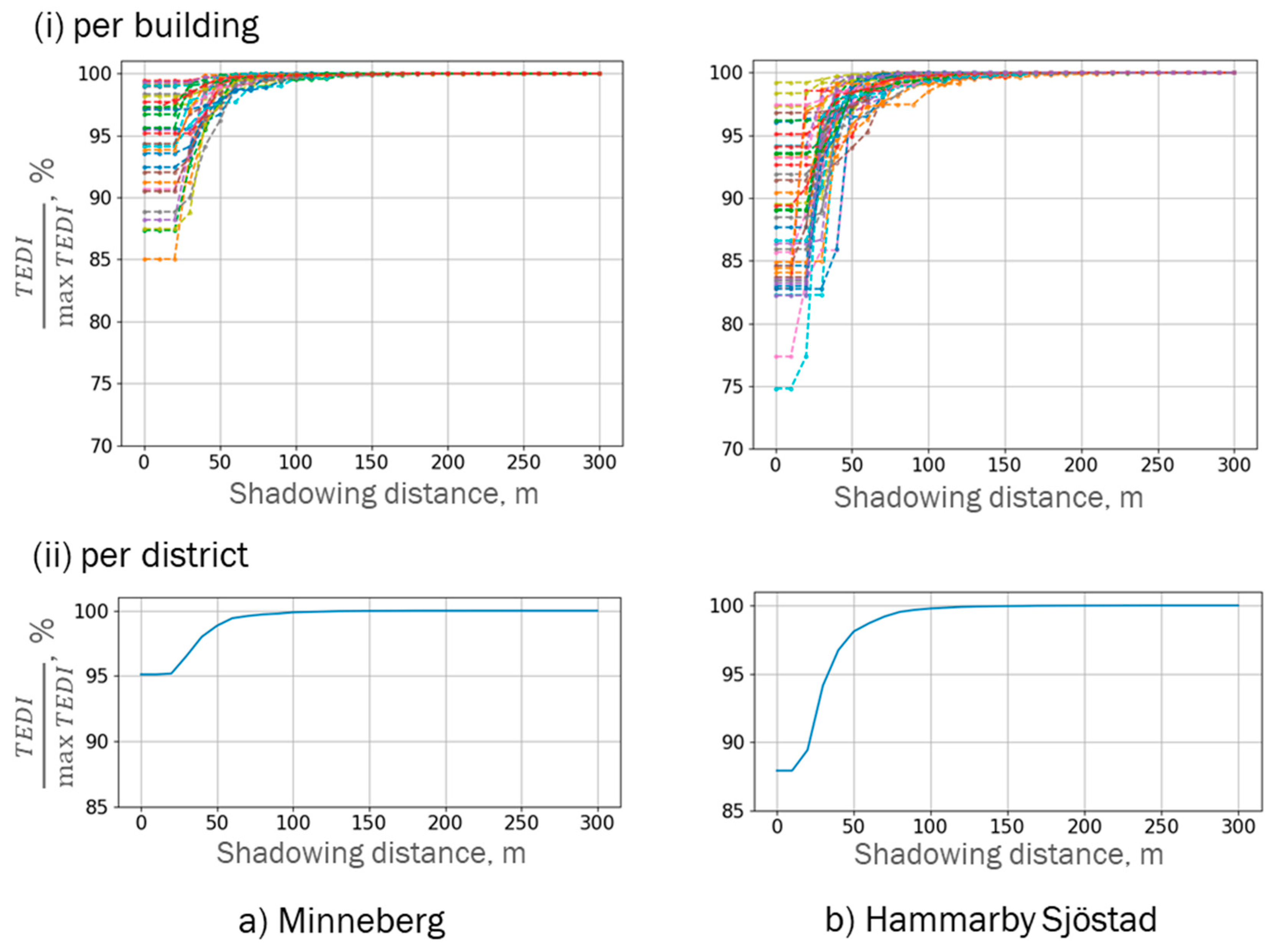
Surrounding shadowing environment. Up to 12% of $\Delta \mathrm{TEDI}$ could be attributed to the change in the shadowing environment in the case of two districts with quite different types of building geometries, with a monotone increase in TEDI along with the increase in the shadowing distance threshold. At the district scale, limited effects (below 2%) were observed for the nearest shadowing environment (up to 50 m). Furthermore, surfaces farther than 100 m did not have any profound effect at the district scale for both studied areas. At the building scale, the limited effects’ threshold rose to 150 m. However, as extra computing time is negligible, the authors would advise keeping 200 m for all simulations.

We conclude that the analysed modeller assumptions embedded in UBEMs have a distinct impact on the UBEMs’ outcome and suggest promoting more explicit documentation of these choices in upcoming UBEM studies.