
Benchmarking Approaches for Assessing the Performance of Building Control Strategies: A Review


1
Bosch Thermotechnology GmbH, Junkersstraße 20-24, 73243 Wernau, Germany
2
INATECH Department of Sustainable Systems Engineering, Freiburg University, Emmy-Noether-Straße 2, 79110 Freiburg, Germany
*
Author to whom correspondence should be addressed.
Energies 2022, 15(4), 1270; https://doi.org/10.3390/en15041270
Submission received: 13 December 2021
/
Revised: 25 January 2022
/
Accepted: 3 February 2022
/
Published: 9 February 2022
(This article belongs to the Topic Sustainable Built Environment)
Abstract
:In the last few decades, researchers have shown that advanced building controllers can reduce energy consumption without negatively impacting occupants’ wellbeing and help to manage building systems, which are becoming increasingly complex. Nevertheless, the lack of benefit awareness and demonstration projects undermines stakeholders’ trust, justifying the reluctance to approve new controls in the industry. Therefore, it is necessary to support the development of controls through solid arguments testifying to the performance gain that can be achieved. However, the absence of standardized and systematic testing methods limits the generalization of results and the ability to make fair cross-study comparisons. This study presents an overview of the different benchmarking approaches used to assess control performance. Our goal is to highlight trends, limitations, and controversies through analytics to support the definition of best practices, which remains a widely discussed topic in this research area. We aim to focus on simulation-based benchmarking, which is regarded as a promising solution to overcome the time and cost requirements related to field or hardware-in-the-loop testing. We identify and investigate four key steps relating to virtual benchmarking: defining the key performance indicators, specifying the reference control, characterizing the test scenarios, and post-processing the results. This work confirmed the expected heterogeneity, underlined recurrent features with the help of analytics, and recognized limits and open challenges.
1. Introduction
Since the dawn of human history, the main purpose of buildings has been to shelter people from the weather. Today, they also serve several other needs—e.g., acting as living and working places—with people now spending an average of 80–90% of their daily time indoors [1,2]. Bearing this in mind, it is unsurprising that the whole building sector accounts for 33% of the global total energy use [3], representing “a source of enormous untapped efficiency potential” (IEA [4], 2021, Buildings—A source of enormous untapped efficiency potential). In the future, time spent indoors is likely to increase further due to a higher occurrence of adverse weather events triggered by climate change [5]. Moreover, because of the growth of the world’s population, the areas covered by buildings are growing larger. Therefore, decarbonizing the building sector, which is responsible for nearly 40% of energy-related carbon dioxide emissions [4], is a target accepted worldwide for limiting climate change [6].
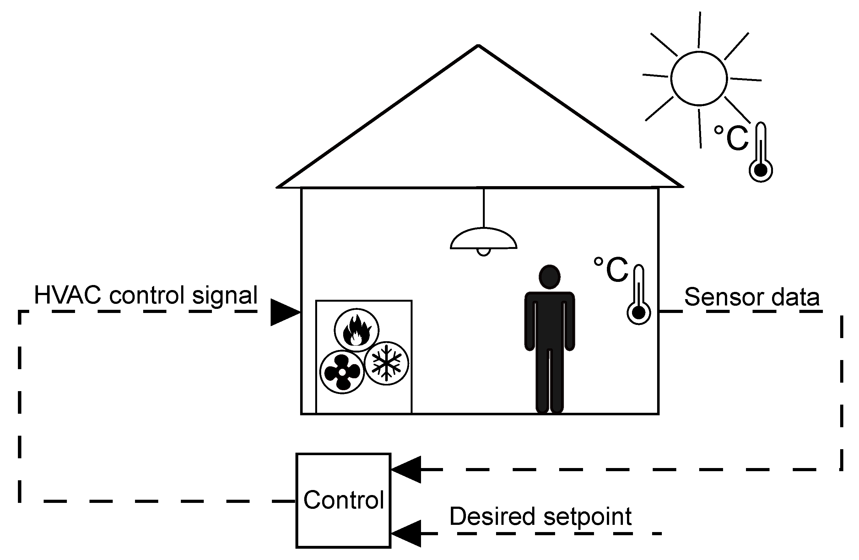
Applying energy efficiency measures to heating, ventilation, and air conditioning (HVAC) systems has greater savings potential than applying measures to other building loads [7]. Compared to the latter (e.g., water heating, lighting, and home appliances), HVAC systems account for around 50% of the total energy consumption of buildings [7,8,9,10]. Three main strategies can be used to reduce HVAC energy consumption: (1) improving the building’s envelope insulation and shading systems, (2) increasing the performance of the best available technology and introducing new heating system technologies, and (3) developing advanced HVAC control strategies. While the first two require a lengthy renovation period, the third is relatively inexpensive and capable of even higher energy savings [7,11], though it has not been emphasized by policies [9]. Moreover, considering the already outstanding performance of system components and the efficiency boundaries, the development of advanced controllers is a frequent aim of research. In particular, researchers are focusing their efforts on developing controls that can handle the expanding complexity of building systems, which will become more interconnected with the grid over time [12,13]. That said, new controls are not solely aimed at reducing energy consumption while guaranteeing occupants’ comfort [14,15,16,17], but also at the effective management of the system given the requirements of providing grid stability and reliability (i.e., peak shaving or load shifting) [12,18,19]. Eventually, the aim is to avoid renewable supply curtailment, thus enhancing the penetration of green resources [20,21,22]. Figure 1 shows a simple schematic describing the working principle of a typical building control system.
While the importance of new control strategies is recognized within academia, their approval at the industry level remains limited, especially with regard to advanced control systems [13,23,24,25]. Several obstacles to the approval of any new green building technology, as outlined in [26], are the lack of awareness of the benefits of these technologies, their risks, the uncertainties involved in their adoption, and the lack of demonstration projects. Moreover, Ouf et al. [27] linked the low level of implementation of occupant-centric controls (OCC) not only to cost hurdles, but also to the limited generalization capabilities of control performance. These arguments demonstrate that there is a lack of confidence in newly developed technologies, despite their usefulness being recognized by practitioners. Therefore, there is the need to provide solid arguments testifying to the performance of control strategies [23,28]. Nevertheless, newly developed controls are often tested and benchmarked while ignoring this need. Additionally, researchers tend to investigate only one specific building application or a few case studies, which differ greatly from study to study, and do not take into account the variations in markets around the globe [22]. In turn, this limits the ability to generalize and compare solutions, justifying stakeholders’ lack of trust.
Multiple review papers have qualitatively evaluated the testing methodologies used to assess specific advanced controls (i.e., model predictive control (MPC) [13,20,24], reinforcement learning control (RLC) [25], and occupant-centric control (OCC) [29]). All these authors [13,20,24,25,29] have reported the absence of standardized evaluation approaches, which prevents fair cross-study comparisons from being made. Both Drgoňa et al. [24] and Afram et al. [20] underline how the key performance indicators (KPIs) used vary from study to study. Moreover, Drgoňa et al. [24] stress that the KPIs used for comparing MPCs should include not only energy and cost savings but also other quantities, such as implementation effort. Additionally, the diversity and shortfalls of KPIs are presented in Stopps et al. [29] for OCCs. Interestingly, in [29], the authors underline that tests are conducted on too-small subsets of residential building typologies, making them unable to represent realistic markets (i.e., little test coverage). The need to test controls on a wider range of buildings is also discussed in [30]. Heterogeneity characterizes not only KPIs and building typologies but also the behaviors of occupants [27,29], the testing locations, and the baselines used for comparison [25]. Canteli et al. [21] state that, in some cases, it can be difficult to understand how tests have been conducted. Concerning this last observation, Beiranvand et al. [31] argue that comprehensive and detailed reports are necessary to ensure experiments’ reproducibility.
To target these gaps, some authors have focused on the development of publicly available virtual testing frameworks, such as the BOPTEST [23] and CityLearn [21]. BOPTEST aims to offer reference test cases, each representative of a specific building typology, location, and user behavior, in order to test developed controls unambiguously on a common platform. CityLearn is a platform that allows the easy implementation of reinforcement learning algorithms for demand response applications in districts [21]. Through this platform, developers can virtually test and benchmark developed RL agents against others RLCs or a rule-based control (RBC), relying on the working principle of the OpenAI Gym Environment. Recently, Wölfle et al. [22] created a guide to develop virtual environments to benchmark the performance of building optimization algorithms. The idea is that once an environment is defined, it is loaded onto a publicly available database, thus enhancing the model reusability, mitigating the lack of standardized testing, and reflecting the variability of realistic scenarios [22].
The concepts discussed above focus on providing a pool of reference test scenarios to ensure fair cross-study comparisons. Nevertheless, it is still the case that little effort has been made to develop methodologies that can ensure a sufficient test coverage addressing the real size and variety of the market (i.e., tackling control robustness). Furthermore, encouraging practitioners to utilize public platforms or contribute to database samples can be difficult, and database maintenance is critical to ensure that environments are trustable. Only part of the outlined gap has been addressed. We believe that test coverage is of paramount importance to allow for performance generalization; enhance stakeholders’ trust; and avoid the risk of predicting, by simulation, misleadingly good behaviors.
This study aims at providing a review that focuses on the different benchmarking approaches used to assess the performance of building controllers. Our goal is to highlight trends, limitations, and controversies through analytics to support the definition of standardized practices and robust testing concepts, which are discussed topics in this research area. Consequently, this work intends to answer the following guiding questions: (1) How are test benches for building controllers defined (i.e., identify key steps to be covered and their requirements)? (2) Can prevailing features and controversies in the approaches be identified to further analyze the heterogeneity already reported by the above-presented authors? (3) Are there special benchmarking needs depending on the type of control tested?
For this, we will focus exclusively on simulation-based approaches. Despite the high trust requirements, simulation-based testing is regarded as a promising solution to overcome obstacles related to time, cost, and repeatability induced by field and hardware-in-the-loop tests (see Section 2.2).
The paper is structured as follows. In Section 2.1 and Section 2.2, we provide some introductory concepts relating to the major control strategies and the prevailing approaches to their testing. Section 3 describes the methodology adopted in this study, while Section 4 presents an in-depth analysis of the reviewed contributions. The results, discussion, and conclusion are given in Section 5 and Section 6.
2. Introductory Concepts
2.1. Building Control Strategies
This section briefly discusses the major control strategies applied to buildings. Based on [2,9,14,15,16,20], we identified two categories, classical and advanced, according to the core operational principle of the controls.
2.1.1. Classical Controls
On–off controls are adopted in the simplest architectures and represent the classical control par excellence. Their working principle is discontinuous and their output signal can be one (on) or zero (off). As a result of this functioning, they are associated with a dead band to account for system time lags and inertia [9]. Nevertheless, this feature is insufficient to avoid overshooting. That is why, together with their static behavior, they lead to a high energy consumption [14]. Consequently, P, PI, and PID controls have replaced on–off systems in several applications. These controls can account for the dynamic response of controlled quantities. However, to ensure efficient functioning, they require the proper tuning of the parameters [32,33]. This prerequisite is crucial [2] and, if not properly accomplished, can induce instabilities [34], which trigger discomfort and energy waste. Nevertheless, thanks to their simplicity and cost-effectiveness [9], a typical control system architecture exploits on–off, PI, or PID as low-level controllers, on top of which a higher-level controller can tackle efficiency and/or optimization [9,10,35].
Among classical controls, we also include so-called rule-based controls (RBC), which are high-level controls [12,36]. These controls rely on a set of predefined if–then rules to overwrite the set points of the system and improve the occupants’ comfort or energy efficiency. The simplest example is temperature set-back rules that, by relying on the defined points of the day, change the set points to lower levels. Ma et al. [37] state that in most regular buildings, the temperature set points are modified when the building is unoccupied or during the night.
2.1.2. Advanced Controls
Classical controls are too simple to target the increasing complexity of building systems, which are becoming more linked to the grid [38] and more intricate due to the presence of multiple energy sources [25]. These complexities require controls able to target multiple, and often conflicting, objectives: they must not only be able to reduce the energy consumption but also strive to guarantee occupants’ comfort, the system’s flexibility, and self-consumption.
To solve this challenge, advanced controls have been widely developed [13]. These controls can solve optimization problems to, e.g., compute temperature set points [17]; predict the energy load by means of building models and, accordingly, manage the system [20]; adapt to occupant variations [27]; and exploit thermal (both active and passive) and electric storage to enhance flexibility [39,40].
One of the distinguishing features of advanced controls is their proactive, rather than reactive, role. As stated by Preglej et al. [41], advanced controls take anticipatory actions rather than corrective ones. Another characteristic element is their “smartness”. Providing advanced controls with some level of computational intelligence (CI) is a topic of great interest in this research area. According to Ahmad et al. [8], some of the most common CI techniques for HVAC in academia are fuzzy logic [33,42], neural networks [7,43,44,45], and genetic algorithms [46]. Other advanced strategies make use of the multi-agent concept, which is based on the maxim of “divide and conquer” [8], according to which a complex optimization problem, or generally any complex task, can be better managed when handled by more actors [47]. Wang et al. [25] highlight the growing research interest in databased controls such as reinforcement learning control (RLC), which is a promising means to overcome the obstacle, introduced by model predictive controls (MPCs), of developing a prediction model. RLCs are based on the concept of learning agents; hence, the control learns how to behave in its environment through appropriate rewards. Additionally, a non-negligible benefit of intelligent controls is their ability to manage the subjectivity of occupants’ perceptions more effectively [2]. In this regard, occupant-centric controls (OCCs) have been developed [29] and are currently covered under IEA EBC Task 79 [48].
In this study, we aimed to use an assortment of the above-mentioned controls to detect the prevailing procedures or common testing requirements. This intent considers the need to develop standardized approaches for systematically testing new controls.
2.2. Approaches to Control Testing
There are three established methodologies that are used to assess the performance of building control strategies: field testing, emulation, and simulation [49,50].
Field testing is considered onerous in terms of both time and cost [29]. Moreover, it implies the engagement of the building user [29], potentially causes discomfort [51], and has been associated with safety risks [28]. Although in situ tests handle real monitoring data and account for all interactions (i.e., no simplifications are introduced) [29], they prevent a fair comparison of different control strategies as it would be nearly impossible to reproduce the input signals [13].
Emulator-based testing allows verifying the control software and hardware in a test rig without the need to set up a complete field test. All the boundary conditions (e.g., comprising the building and its system, the user behavior, and the climatic profiles) are emulated through real-time simulations that ensure the reproducibility of experiments. This testing approach is independent of the building user and the safety risks associated with field testing. Moreover, the cost and time requirements are reduced, albeit still present (i.e., constrained to real-time simulations [34], laboratory equipment), while ensuring the testing of the tangible components that will be installed later.
Simulation-based testing replaces the software and hardware parts in emulations with a simulation model. This model represents the time-evolution of the real system. A fully virtual approach not only minimizes the testing costs, avoiding the need for the installation of any instruments or appliances [52], but also enables the optimization of the design, detecting errors before field implementation, and accelerating the testing procedure, as the real and simulation clocks can be fully decoupled. In 1985, Hirsch et al. [53] highlighted the potential of a simulation-based approach and recognized it as the only practical way to analyze the performance of any technology targeting energy efficiency under a wide range of scenarios. Nevertheless, the reliability of virtual approaches is strongly linked to the accuracy of the simulation model, which represents a common issue in building simulation. This is due to the significant difference between the measured and simulated building energy performance [54]. Model development usually requires skilled practitioners and a considerable amount of time. Additionally, capturing the perceived occupants’ comfort in a virtual environment presents several challenges [29]. Time might remain a constraint due to computational speed.
Although these three approaches should be regarded as complementary [2], this study investigates purely simulation-based tests. These are considered to be promising solutions for assessing different control strategies at an early stage and ensuring test coverage. Moreover, high-quality virtual environments can be used by practitioners to perform virtual release tests when minor updates to a previous control strategy are introduced.
3. Methodology
We conducted this review based on the Scopus and Science Direct databases. Defining appropriate selection criteria for the targeted aim is not a trivial task; on the one hand, researchers usually append some level of performance comparison to the development of any new building control strategy. This statement implies that the number of contributions that need to be analyzed could be too large to handle. On the other hand, the majority of publications do not explicitly refer to virtual testing or benchmarking but rather to new control attributes. Therefore, the researched keywords were not solely testing and benchmarking but also simulation, comparison, baseline, on–off, traditional control, PID, and rule-based. These terms were combined with the following ones: building control, HVAC control, building, residential, home, commercial, control strategies, control system, and room control. Thus, complex scanning criteria were generated. This study relied on the inclusion and exclusion criteria listed below, which were reflected in the search terms adopted.
- Findings should present, test, and benchmark a new building control strategy or describe in detail a virtual benchmarking framework. This review focuses on the applications of new controllers to residential and fully enclosed commercial buildings.
- The field of application excludes lighting, window openings, shading operation, domestic hot water preparation, and smart grid frameworks. The focus is on high-level (i.e., supervisory) controllers; hence, low-level controllers are out of the scope of this review.
- As the focus is on simulation-based testing, contributions that present emulation or field experiments are disregarded.
- If for the same year, several in-scope-contributions are identified, those with a higher number of citations are prioritized.
Scopus and Science Direct were accessed in January and April 2021.
We have further reviewed the database of the conference proceedings of the International Building Performance Simulation Association (IBPSA) [55]. The international conference reveals the major outcomes of the world’s leading research community on building modeling and simulation. The first contribution related to control strategies appeared in 1989 for fault detection identification. From 1991, controls for heating systems and energy management systems have been discussed.
To ensure the depth of coverage and variety of the investigated sample, we have selected a few relevant papers from the reviews of [25] on reinforcement learning control (RLC) and [20] as well as [24] on model predictive control (MPC). The selection criteria for this second literature identification are equal to those adopted for the database analysis.
Based on the defined inclusion and exclusion criteria, the number of relevant papers selected resulted to be 50 (i.e., we roughly reduced the findings to a quarter).
Figure 2 provides an overview of the paper that summarizes the methodology adopted.
4. Results
This study identifies and investigates four key steps that characterize simulation-based benchmarking. Section 4.1 describes the key performance indicators (KPIs) computed for the evaluation of controls. In Section 4.2, we discuss the reference control defined for comparative purposes. Section 4.3 reports how the virtual test scenarios are specified, while Section 4.4 discloses how the benchmarking results are visualized and documented.
We grouped the control strategies into five classes; these are fuzzy logic controls (FLC), generic advanced controls (GAC), model predictive controls (MPC), reinforcement learning controls (RLC), and traditional controls (TRC). The cluster GAC includes optimal, occupant-centric (OCC), and agent-based controls. As highlighted in [9], few publications present improved features compared to classical control strategies, which explains the significant presence of advanced controls in this study. During the research, we noticed that contributions could mainly be grouped into two predominant fields: model-based predictive controls and databased controls, especially RLC.
Table A1, in Appendix A, shows the main information of the reviewed papers.
4.1. Key Performance Indicators
The primary outcomes of testing are the KPIs, which quantitatively assess the performance of the investigated control strategies. As stated by [12], an appropriate selection of evaluation metrics is necessary in order to guide the design of new controllers, as it guarantees that needs, expectations, and requirements are fulfilled. Generally, the developer sets the required KPIs to target the main features of the new strategy [49]. This is why testing approaches are prone to being case-study-oriented, preventing standardization and limiting quality, because developers may exaggerate the benefits of their newly devised control.
In light of the above, it is unsurprising that the KPIs presented in the reviewed papers are largely heterogeneous. Nevertheless, we identified three recurring domains that quantify energy consumption, occupants’ thermal comfort, and energy cost. Figure 3 depicts the share of the total KPIs collected in this study (i.e., 245) based on these domains. The tag others applies to metrics that cannot be assigned to any of the three. For example, this category includes the flexibility [39], exergy [56], PV self-consumption [57], and carbon dioxide emissions [58] metrics.
4.1.1. Energy Consumption Metrics
It is noteworthy that an energy consumption metric is computed in 84% of the contributions and represents 39% of the total KPIs. This is because reducing the buildings’ energy demand and the corresponding CO2 emissions is one of the primary drivers in the development of new controllers. Among the eight contributions that do not present an energy consumption metric, Refs. [43,46,59,60] compute an energy cost metric, Dermardiros et al. [61] depict the intermittent operation of the heat source, and Refs. [33,62] focus on occupants’ thermal comfort. Glorennec et al. [42] compare the obtained fuzzy logic control rules table with the specified baseline table.
The energy consumption is quantified either as total kilowatt-hour () or specific (per unit of heated/cooled surface). The computation of the first prevails over the latter (computed by seven contributions—14%). Nevertheless, the specific energy consumption is preferable for benchmarking, as it is not biased by the building size.
In some cases [2,57,63,64,65,66], the energy consumption is provided as both total and partial: energy consumption is listed for the relevant components of the heating, ventilation, and air conditioning (HVAC) system or separately for space heating and cooling.
Another approach is to compute the energy savings, which are quantified as a percentage (or improvement) of the consumption reduction compared to the specified reference, as in [18,36,47,58,65,66,67,68,69,70,71,72,73]. Note that Refs. [47,58,65,67,69,70,71,72,73] quantify both the energy consumption and the energy savings. Whether the computed energy is primary is not discussed, except by [63,64,72,74]. However, the lack of energy conversion factors suggests that the studies disregard the energy share related to the conversion processes, thus accounting solely for the thermal or electrical energy carriers. The primary energy consumption describes the needs of the building more thoroughly and also allows for the comparison of multiple generation units that are fueled by different sources. Nevertheless, the adoption of this metric can hinder performance comparability when dissimilar conversion factors are specified. These values are defined at national levels and vary considerably, as they are influenced by multiple grid characteristics (i.e., energy mixes, production sites, and distribution networks), and, often, political choices.
Energy metrics require the specification of a time horizon. This temporal duration typically corresponds to the test duration, which greatly varies among publications (see Section 4.3.2) and is usually as long as one year. When energy consumption is computed over different time horizons, comparisons of results can be misleading.
4.1.2. Thermal Comfort Metrics
Other than energy consumption, the influence of control strategies on occupants’ wellbeing is considered by two-thirds of the investigated contributions. Furthermore, Figure 2 shows that 26% of all computed KPIs belong to the thermal comfort domain.
Although several KPIs can be used to quantify thermal sensations [75], the majority of the reviewed papers adopt Fanger’s metrics: the predicted mean vote (PMV) and the predicted percentage of dissatisfied (PPD). In particular, multiple authors [2,11,36,47,69,76,77] compute the average PMV or PPD, albeit they describe occupants’ comfort only in a general way [77]. It is worth noting that Klein et al. [47] introduce a metric that estimates discomfort at the level of individual occupants through the implementation of a human agent [47]. These authors compare their metric to the average PMV and conclude that their approach leads to more accurate results [47].
The PMV ranges on a dimensionless scale sensation from −3 (cold) to +3 (hot) and is computed by determining the steady-state heat balance between the human body and the environment. According to the reference standards ISO 7730 [78] and ANSI/ASHRAE 55 [79], an occupant feels comfortable when the PMV ranges between −0.5 and +0.5 (i.e., category B). Note that category B is selected in every contribution except for [80], which adopts the more severe requirements of category A (i.e., −0.2 and +0.2). The PMV is a function of the clothing insulation, level of body activity, air velocity, and humidity, as well as air temperature and mean radiant temperature [75].
The parameters used for describing occupants are typically defined based on norm prescriptions and tend to be constant during the simulation; for instance, clothing insulation is typically set to be equal to 1 clo ( m2K/W) in winter and clo in summer, as in [45]. Nevertheless, heterogeneity in the definition of these values is evident. For instance, Zhao et al. [69] define 1 clo in winter but clo in summer, differently from Zhang et al. [67], who use clo and clo, respectively. Additionally, Egilegor et al. [62] assume clo during cooling mode and clo for heating. Moreover, Ascione et al. [60] set a clothing resistance of clo at night to account for blankets, whereas Garnier et al. [76] define a variable resistance based on the outside temperature at 6 a.m., modeling the influence of the outdoor temperature on the clothing thickness. Furthermore, Chen et al. [40] set a two-level resistance profile equal to clo during the first two simulated days and raised it to clo for the remainder.
Fixed values are also specified for the physical quantities, such as the air velocity (e.g., m/s in [69], m/s in [40], m/s in [67,80]) and humidity (e.g., 40% in [47] are 50% in [80]). The heterogeneity of these parameters may prevent fair comparisons being made between tests.
The PPD is a percentage value that quantifies the amount of thermally dissatisfied individuals in a large group [75]. Showing the statistical distribution of the PMV [77], its evaluation indirectly requires defining the same occupant and physical parameters of the PMV. The comfort PMV range of ±0.5 implies a PPD smaller than 10%. Ranging from 0% to 100%, this metric has the advantage of being minimized [60].
Although PMV and PPD are metrics that are accepted by the reference standards [2], their validity is questioned. For instance, Fazenda et al. [81] state that adaptive comfort models should be preferred because they do not rely on fixed parameters. Moreover, Fanger’s model can be applied to conditioned buildings, which ensure the required steady-state assumption, and it can only be used for healthy adults. If these conditions are not met, the results will not reliably show occupants’ sensations [75]. In this regard, Chen et al. [40] evaluate not only the PMV but also the actual mean vote. The latter is defined by the authors as the sum of the PMV and random white noise, which follows a Gaussian distribution. If the noise is greater than 0, the PMV underestimates the actual mean vote, and vice versa when it is smaller [40].
Another typical approach is to quantify thermal comfort based on the difference in the room temperature from the set point, or from a temperature range, which is defined as a tolerated temperature difference across the desired set point (e.g., ±1 K [82]). This difference is quantified in several methods by computing the temperature root-mean-square error (RMSE) with respect to the set point or the upper and lower temperature limits [39,64], the temperature deviation [82], the frequency (i.e., numbers of values in a bin of K) [72], the percentage of time spent inside the comfort temperature ranges [35,83], the temperature mean-bias error and the coefficient of variation of the temperature root-mean-square error [68], the number of violations [74], the amount of violation (in ) [74,84], or the average temperature deviation [70]. Yu et al. [85] define the discomfort cost in as a function of the squared temperature deviation from the set point, whereas Anastasiadi et al. [2] express the ratio of time spent in discomfort to the total time (in percentage).
On the one hand, disregarding any comfort model, this second approach is straightforward and makes comparisons easier; the presented KPIs do not depend on many parameters. On the other hand, this approach might be unable to model human thermal sensations in sufficient detail. Therefore, it could be used in combination with more detailed metrics (e.g., following a hybrid approach). A possible solution would be to weigh the discomfort time according to the ratio of the actual PPD and the comfort threshold (e.g., ) [78], as in [80]. Moreover, defining the desired temperature range is not trivial, since thermal sensations tend to vary among users. A solution to this would be to define comfort ranges at least for two extreme cases—tolerant and intolerant occupants—which is similar to [27].
It is noteworthy that Ouf et al. [27] evaluate the thermal comfort, guaranteed by the developed occupant-centric control, through the quantification of occupant interactions with the building or overrides. These are expressed as the frequency of pressing the thermostat and light switches each year. Eventually, for energy consumption metrics, the same experiment duration must be used to enable to consistently compare the results. This observation also holds for the metrics presented in the sections that follow.
4.1.3. Energy Cost Metrics
Some test benches, such as [11,18,39,43,46,57,58,59,60,66,77,83,85,86,87], assess not solely the energy consumption and the thermal comfort but also the energy cost. In total, 16% of all KPIs belong to the energy cost category (see Figure 3).
The latter is computed as a product of the energy required and the electricity or gas price, depending on the generation unit used. It is noteworthy that in the analyzed contributions, the generation unit is typically fueled by electricity. This observation is supported by the fact that advanced controls, which strive to reduce the energy costs given a variable price signal, allow researchers to implement demand response systems [88].
Three types of tariffs are present: constant [46,60]; time of use, which typically has two price levels (e.g., day/night [11,77], peak/off-peak [18,59]); and dynamic [39,58,73,86,87]. When these tariffs are adopted, the forecast time is equal to one day, except for McKee et al. [43], who implement a minutes-ahead profile, or is assumed to be in real time [58,86].
Prices are an external input for all studies. For instance, Pereira et al. [66] adopted the Portuguese tariff scenarios. Therefore, standardization might be enhanced by defining a set of references for the price scenarios and providing a clear reminder of the data source, ensuring ease of access to any user.
Normally, the developers will test only one price scenario. Nevertheless, in [59,88], the authors adopt two tariffs: a peak and off-peak tariff and a highly time-varying one. In particular, Vrettos et al. [88] compare an MPC to an RBC both in the case of a day/night tariff and a predefined dynamic tariff (day-ahead). The second allowed a greater load-shifting capability.
Regarding the energy consumption, the energy cost is also quantified as savings with respect to the specified reference (e.g., [11,73,88]).
Since the potential for financial savings is a driving catalyst for adopting new technologies [22], energy cost indicators are regarded as meaningful KPIs that should ordinarily be included, as well as when demand response is disregarded. Moreover, the computation of a metric, such as the net present value, could be effectively adopted to justify the initial costs required for adopting new controls, provided future savings are possible.
4.1.4. Other Metrics
The three metric domains presented above can be considered essential in any testing and benchmarking approach. Nevertheless, besides this so-called standard KPI set, other indicators are adopted to assess other control attributes. Figure 3 highlights that 19% of the collected KPIs do not belong to the standard KPI set.
Flexibility metrics are a good example. These indicators evaluate the interactions between the building and the grid [12]. Hu et al. [39] define and benchmark the flexibility factor to determine the ability to shift the energy consumption from peak to off-peak hours [39]. Salpakari et al. [86] evaluate the building energy flexibility by computing the annual grid feed-in and the annual electricity balance. Another metric that can be related to flexibility is the PV self-consumption, which is quantified in both [57,87]. The latter can be used to quantify the use of renewable electricity [57].
Other than these flexibility metrics, multiple authors define additional KPIs at the system level. For example, Maasoumy et al. [89] compute the total airflow rate () and peak flow rate (). Fischer et al. [57] quantify the backup heater usage as the total operating hours, and the heat pump usage through the mean part load ratio and the numbers of unit toggling. The latter is also adopted in [61]. Both Refs. [58,83] evaluate the coefficient of performance of the heat pump. Additionally, Kubot et al. [83] evaluate the PV curtailment and the battery state of charge, whereas Ruusu et al. [58] compute the average tank temperature in three positions (upper, middle, and lower).
Another metric used is the exergy loss (e.g., [64,90]). For performing an exergy analysis, a reference environment—typically the outdoor dry-bulb temperature—needs to be defined [64]. Both Refs. [64,90] adopt the use of ambient temperature.
It is worth noting that Ruusu et al. [58] quantify the carbon dioxide emissions, in kilograms, through specified factors () for the electric and thermal grids, based on Finnish data from 2015. Mossolly et al. [46] evaluated the percentage of time the room CO2 concentration () is within three ranges (i.e., less than 770 ppm, between 700 ppm and 1000 ppm, and more than 1000 ppm). Furthermore, Refs. [76,87,89] compared the simulation time.
Heating, lighting, and cooling utilization ratios quantifying the energy use, based on the number of occupants, were computed in [27] to test the performance of an occupant-centric control (OCC). By the adoption of OCCs, the control adapts to the occupants; hence, the utilization ratio should decrease.
4.1.5. Number of Computed KPIs
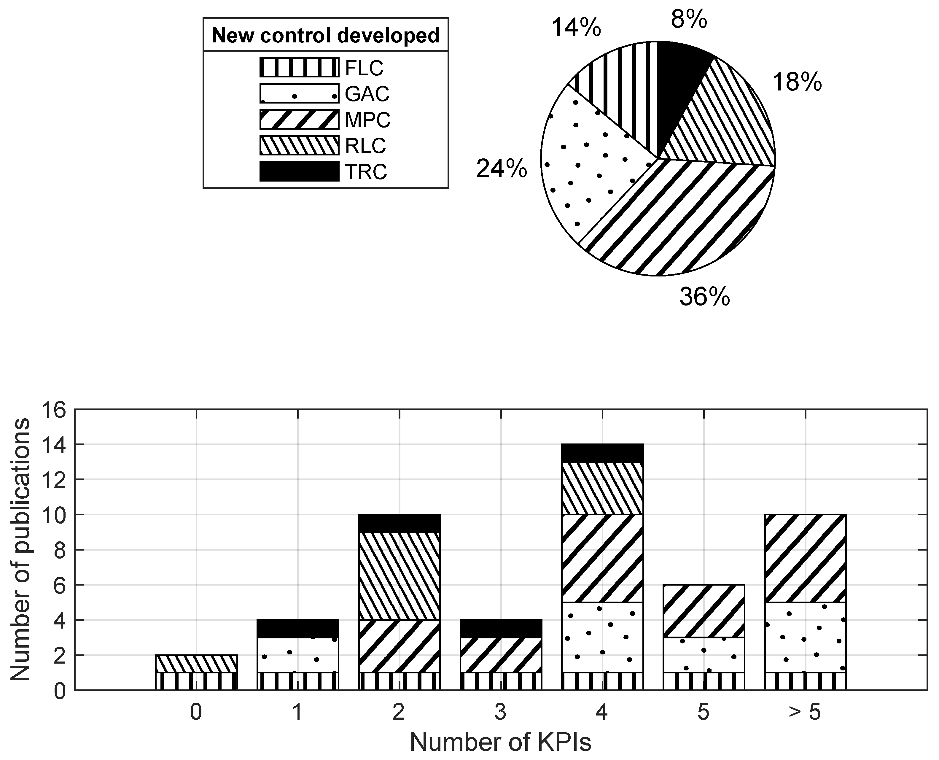
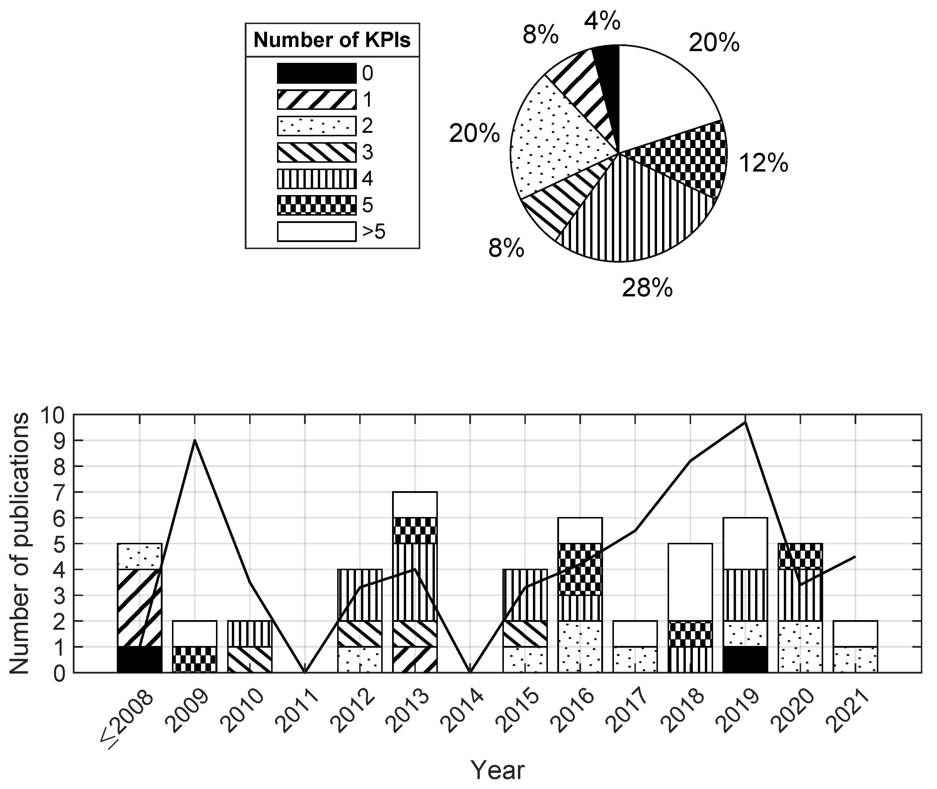
Figure 4 shows the number of KPIs computed in each analyzed contribution, whereas Figure 5 highlights the number of KPIs adopted for year of publication, from the oldest identified paper published in 1991 to the newest in 2021.
Figure 4 reveals that the preferred number of KPIs is four.
Accordingly, Figure 5 shows that there is a slightly more marked tendency to adopt four KPIs: 28%. Of the remaining, 20% computes two metrics, and another 20% computes more than five. It must be noted that these indicators mainly belong to the energy consumption and thermal comfort domains, as has already been mentioned in Section 4.1.2. This implies that these studies present more than one energy and comfort metric (e.g., both the average PMV and PPD, or both energy consumption and savings). The highest metric value—i.e., 36—occurs in [58].
It is noteworthy that Dermardiros et al. [61] and Gouda et al. [33] do not compute any KPIs. Rather, the first benchmark is the room temperature and the operation of the heat source profiles, while the second compares the control rule tables.
Evidence of a clear trend in the computed KPIs, based on the control type, is absent. Nonetheless, some recurrences can be identified: (1) an energy cost metric is present mainly for controls that target demand response; (2) occupant-centric controls rely heavily on thermal comfort assessment, following advanced metrics such as those that measure occupants’ interactions [27] or the actual mean vote [40]; (3) observations of the RLC behavior during the learning time are commonly reported, as they represent the weakness of RLCs. RLCs typically disregard energy cost objectives.
The absence of a consistent tendency in Figure 5 enforces the heterogeneity of the approaches, which is apparent in all the control typologies studied in this review. Despite advanced controls potentially being able to deal with more than two competing objectives, there has not been any marked gain in the increase in the KPIs computed [12]. Interestingly, from 2011 to 2021, the amount of KPIs is always greater than one, except for in Baracu et al. [82], who report only the energy consumption, while comfort is a constraint on the control that is not quantified for comparison. Rather, the room temperature profile is adopted to show that thermal discomfort is absent.
This study reveals the absence of contributions that adopt holistic metrics to enable an easier ranking of the tested control against the specified baseline. The affirmed approach is to discuss the pros and cons of the tested control for each KPI. Later, these observations are summarized together in the Conclusion section and used to decide whether the test has succeeded. Nevertheless, this procedure is manageable when the number of KPIs and tested scenarios is limited. Once these values increase, the amount of data to compare also increases; hence, such a KPI-focused analysis tends to become intractable.
Although holistic metrics are less sensitive to local performances, they can aid in drawing conclusions, especially when significant trade-offs between the defined metrics are expected, inexperienced users are involved, or the amount of data needing to be analyzed is large. Kümpel et al. [77] highlight the need for a metric of this kind. However, suggestions as to how it should be computed are missing. In all the reviewed contributions, the adoption of a KPI-focused analysis is justified because the number of simulated scenarios is small (see Section 4.3); hence, the results used for analysis and benchmarking are manageable.
4.2. Benchmarking Reference
Showing the improvements offered by a new technology over an established one might attract stakeholders. Therefore, the specification of a reference is crucial.
This work identifies three complementary comparison approaches. The new control is benchmarked to either (I) a baseline installed, or assumed to be installed, in existing buildings; (II) an ideal control, which represents the best performance achievable; or (III) a similar control that varies in some features. The second and third approaches alone may be insufficient to spur the adoption of the developed technology. Thus, comparison against a baseline is recommended and is indeed provided in all the analyzed publications.
It should be stressed that the third method allows researchers to test different features of the developed strategy in order to explore which is optimal. For example, Ref. [11] designs and tests various MPCs, which are defined identically but present different weights for computing the cost function.
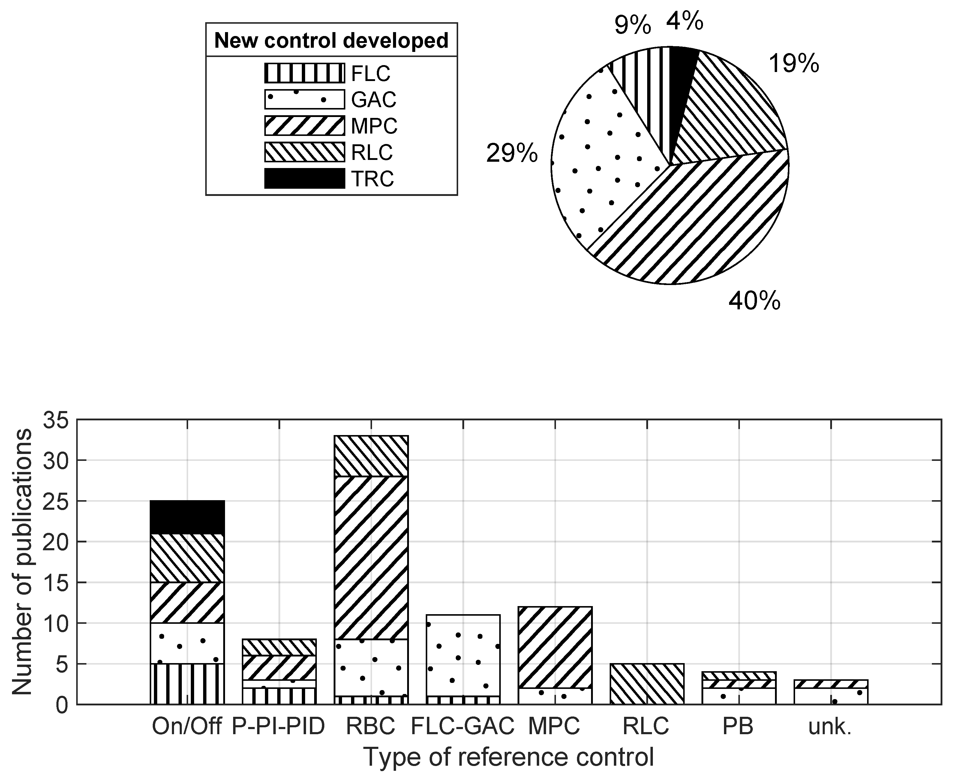
Figure 6 depicts the control typologies used as comparison references. The term on/off refers to controls that maintain the same temperature set point throughout the test, regardless of the state (e.g., [36,43]).
The P-PI-PID tag is assigned to the contributions that adopt proportional, integral, or derivative controls (e.g., [33,61,63]). As described in Section 2.1, these traditional controls require proper parameter tuning to ensure their high performance. Therefore, a tuned control should be adopted, or else the comparison could result in misleading positive improvements [24]. If the set of tuned parameters is not reported (e.g., [17,42]), it will be unclear how well the baseline control is performing. Moreover, ensuring experiment reproducibility can be arduous.
Publications [27,73,89] in which the baseline control is described with little information are put into the category unknown reference control (unk.).
Rule-based controls (RBC), together with on/off, are the ones adopted most as baseline references (see Figure 6), and Refs. [40,68,74,88] affirm their well-established role in building automation. Their supervisory working principle relies on a set of if–then rules that are specified by the developer and mainly act on the temperature set points. These rules are not common to all the investigated contributions and can be very complex [57,58]. Nevertheless, the tendency is to set a simple rule to lower the set points according to the occupancy level (e.g., occupied/unoccupied, weekends, day/night). This approach applies to commercial, office, and residential buildings. These simple RBC rules require not only time schedules but also corresponding set points. In the reviewed papers, the space heating set points vary greatly in the range of 19 to 24 . However, these values should be uniquely defined, considering also the possible thresholds set by national laws. The definition of set points is guided by the desired comfort requirements and can vary from user to user (especially when manually specified). A reliable benchmarking methodology should account for this prospect.
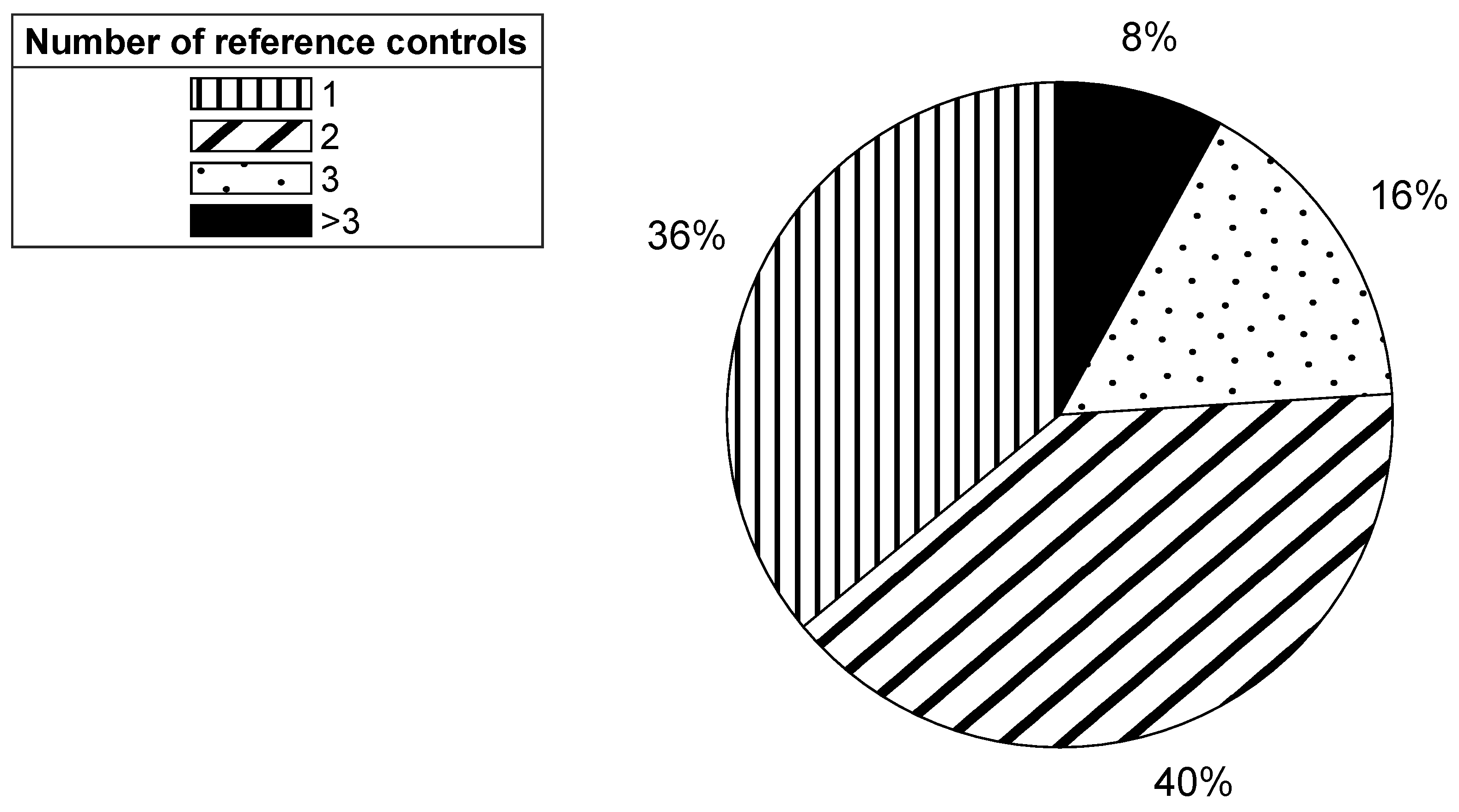
Figure 7 shows that 64% of the contributions adopt more than one reference control. This implies that developers use a combination of the three identified methods, applying either the first and the second or the first and the third. It must be noted that multiple authors [18,61,76,91] rely on two traditional controls (e.g., on/off and RBC) to quantify the improvement gained.
In 36% of the studies analyzed, the authors compare the tested control to just one established control. This outcome is depicted in Figure 6 as well, where the x-axis reports advanced control strategies such as FLC-GAC, MPC, and RLC, as well as the performance bound (PB) represented by ideal controls. For example, Moriyama et al. [92] compare an RLC to an MPC (II approach), proving that a databased approach performs better compared to model-based controls. Egilegor et al. [62] develop and benchmark a standard FLC with an advanced one tuned by a neural network. Moreover, Mbuwir et al. [87] benchmark five RL algorithms with different learning methods. Hazyuk et al. [49] introduce an MPC, ideally capable of perfect predictions, as an upper performance bound to test the new control (i.e., the III approach). A similar method is presented in [56], where the control is benchmarked to a traditional and an ideal operation. Additionally, Oldewurtel et al. [74] adopt a fictitious control capable of perfect predictions as a reference to assess how far the investigated control is from the maximum theoretical performance.
4.3. Virtual Scenarios
Simulation-based benchmarking exploits models of physical phenomena to emulate the entire test environment. Considering building controls, the elements that characterize the virtual test scenarios are the building, its HVAC system, the occupant behavior, and the weather data.
The use of simulations increases the potential of achieving higher test coverage: The tested scenarios can be high in number without involving extra costs, waiting for specific weather conditions, or affecting the occupants. Moreover, models make it possible to increase the flexibility and provide the potential to explore future scenarios. As for field tests, the duration of the test must be defined by the developer. This parameter is relevant for correctly comparing KPIs, as discussed in Section 4.1.1, and to obtain an exhaustive understanding of the control performance. Although simulation-based benchmarking is less time consuming, the test duration and the model complexity can threaten the computation advantage.
This section investigates in detail the approaches used to characterize the virtual scenarios: the test location (Section 4.3.1), the test duration (Section 4.3.2), the building and HVAC simulation models (Section 4.3.3), and the occupancy model (Section 4.3.4).
4.3.1. Test Location
The building site location dictates two fundamental exogenous parameters: the ambient temperature and the solar irradiation. These data, together with the relative humidity and wind velocity, are mandatory inputs in any simulation-based experiment. In addition to the building and system parameters, they form test scenarios and have a great influence on the control performance.
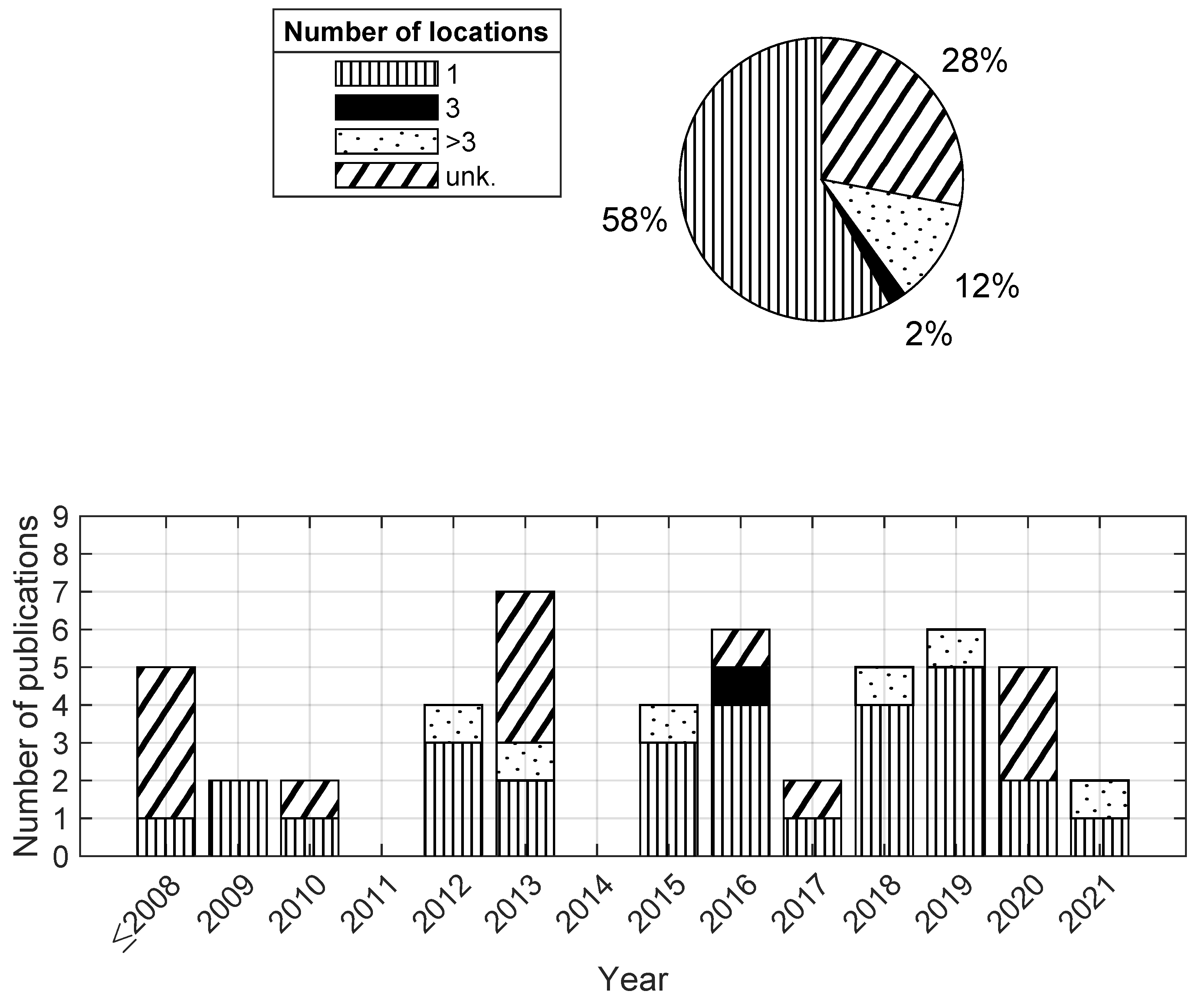
Nevertheless, based on Figure 8, due to the small number of locations, the relevance of these parameters can be disregarded.
Remarkably, 58% of the studies adopt only one location for assessing control performance. In 28% of the publications, the name of the location is not specified (unk.). Of this share, only one contribution, [62], models more than one location.
Despite the results obtained for a single tested location potentially being valid for several similar locations, they cannot ensure a robust performance generalization at the market level, as countries are characterized by multiple climatic zones. Ye et al. [65], who performed a national level analysis, adopt sixteen climatic zones to represent the U.S. market [65].
This limited number of test locations could be related to simulation time constraints. However, none of the contributions refer specifically to computational burden issues, except for [77].
The origin of weather data is sometimes unspecified, making experiment replication nearly impossible. When looking at contributions that report their weather data sources, two major attitudes can be identified. Multiple authors, such as [11,18,61,91], adopt typical meteorological years (TMY) or equivalent weather data obtained over a long period of records (20 to 30 years). Several others adopt measured data available for a site for a specified year—e.g., [58,88,89]. For example, Ruusu et al. [58] rely on data for 2015 provided by the Finnish Meteorological Institute.
Although the latter approach is better able to represent specific local weather and does not rely on averaging, interpolation, or clustering, the data are difficult to share and require either gauging systems or access to weather companies’ data. These requirements increase the time and cost as well as hindering standardization. Furthermore, to improve the standardization of tests, TMYs from a public database such as EnergyPlus [93] would allow the easier sharing of reliable data while guaranteeing access to a vast number of locations with little effort. Extreme days should also be simulated to address the limitations of typical years, which would inevitably lead to describing averaged trends.
4.3.2. Test Duration
The test duration varies across a broad range of operation durations in the order of days, weeks, months, or years (see Figure 9). The tag annual in this study also considers experiments over an entire heating season or cooling season. In 34% of the investigated publications, the developer tests the control operation for one year. Of these, only two groups [27,94] performed a three-year-long experiment.
In the reviewed publications, the selection of a shorter duration is typically not justified. Exceptions are [60,77], where the authors claim for the need to save computational effort and set the duration to a few reference periods. Nonetheless, this is a popular strategy for alleviating the computational burden if the simulation model is slow.
When the number of weather input parameters is reduced, the developer can perform faster experiments at the cost of accuracy: The identification of reference days always introduces simplifications [95]. With the same occurrence of annual tests—34%—another approach is to test the hottest and coldest days recorded in the weather data, or both, as in [40,65,90,96]. Detailed information on how reference days are selected is absent.
4.3.3. Building and HVAC Models
The simulation model used for the building and HVAC systems is of paramount importance in simulation-based tests. Conducting virtual experiments has several advantages (see Section 2.2), as long as the simulation model is sufficiently accurate. Otherwise, the testing results are unreliable.
Three modeling methods are present in the literature: white-, black-, and gray-box models. White-box models consist of a set of mathematical equations that describe mass and energy balances. These physical models are associated with lengthy development times, high computational efforts, and experienced developers. Furthermore, the modeling assumptions introduced affect their accuracy (i.e., sufficiently realistic models). Additionally, white-box models are characterized by a large number of parameters that might be unclear, making them difficult to specify.
Black-box models are data-driven models that correlate input and output measured variables, disregarding any physical process. Compared to white-box techniques, black-box approaches are computationally lighter and more accurate, since assumptions are not required. Nonetheless, they require a sufficient amount of measured data, which is rarely available. Furthermore, being based on measurements from a specific building, model generalization can result in a great loss of accuracy. Moreover, data-driven models might result in unrealistic or even non-physical values, violating, e.g., the law of thermodynamics.
Gray-box (hybrid) models, as the name suggests, combine the above-presented approaches. Their basis is built from physical models (i.e., white-box approach) whose parameters are estimated based on measured data of the system (i.e., black-box approach).
In the reviewed contributions, the prevailing modeling approach is the white one. In particular, 62% of the analyzed articles rely on well-established simulation tools, among which is EnergyPlus [11,97]. Other software, such as Modelica [98]-based environments, TRNSYS [99], and MATLAB/Simulink [100], are also utilized extensively. Several authors use co-simulation frameworks to exploit the potential of two different software products. For instance, EnergyPlus is considered optimal for modeling the building thermodynamics and is combined with a Modelica environment to model the HVAC system and the control [36]. Other combinations are possible: MATLAB/Simulink and TRNSYS (e.g., [39,58,63]) or EnergyPlus (e.g., [18,44,60,69]). MATLAB/Simulink seems to be the preferred tool for implementing control algorithms, especially when optimizations are involved.
The other approach, used in 38% of the analyzed contributions, is to identify a set of physical equations (lumped-capacitance models) instead of adopting computer-aided modeling tools (e.g., [42,61,82,84,85,91]). Simulation tools are also combined with user-developed models, especially for HVAC modeling purposes [58] or for control implementation [46,63,80].
The authors report the models’ accuracy only when the control and the new model are developed together. The validation is performed by comparing the simulation data with the experimental one; excellent agreement of these two is shown. In all other cases, details regarding the validation of the model are not provided. Moreover, the KPIs—i.e., the results of the simulated tests—are not compared to the same metrics, which are calculated based on real data. That said, it is unclear to what extent the accuracy of the simulation model affects the evaluation of the control performance. By reporting the KPIs with their simulation uncertainty, the trustworthiness of simulation-based benchmarking could be improved.
It is worth noting that simplified single-zone models are preferred (58%) to detailed multi-zone identification. In this regard, Goyal et al. [70] stress the need to further verify the assessed control performance for a multi-zone building. Furthermore, Klein et al. [47] state that multi-zone models, as opposed to single-zone models, can represent the complexities of commercial buildings.
The developed model, in the majority of the contributions, emulates a very specific building. For instance, both Refs. [92,101] investigate the application of a control to a data center; Du et al. [90] investigate its application to an airport; and Glorennec et al. [42] investigate its application to a highly glazed building. Moreover, as also highlighted in [29], the tested construction is, in multiple cases, equal to an building affiliated with the authors [33,47,51,89,96]. Nevertheless, the adoption of specific buildings hinders the generalization of the results to different markets. Therefore, it is difficult to perform fair cross-study comparisons and to assess the robustness of the control.
Both Sangi et al. [64] and Ascione et al. [60] remark that their tested building is representative of a typical German and southern Italian construction, respectively. Ascione et al. [60] claim the need for extra studies to assess the full potential of the developed MPC; moreover, Carrascal et al. [84] observe that their results can be used qualitatively for buildings similar to those tested. Additionally, Dermardiros et al. [61] model a typical house in Montreal based on their experience.
The presented approaches imply that controls are rarely tested for different building types and system configurations; hence, only a few case studies test the robustness of the control to varying characteristics (e.g., envelope quality or HVAC configuration). For example, Oldewurtel et al. [74] test different building orientations, window dimensions, and HVAC systems; Fischer et al. [57] account for four different thermal storage sizes; Demardiros et al. [61] consider a system with and without an underfloor heating system to study if the RL agent exploits weather predictions; and Gouda et al. [33] test a building with very low inertia.
4.3.4. Occupancy Model
Despite the increasing focus on guaranteeing occupants’ thermal comfort and the fact that occupant behavior is recognized as the main source of disagreement between simulation predictions and real building operations [102], fixed behavioral schedules are used by developers to test and benchmark new controls. For example, Vrettos et al. [88] assume residential buildings to be occupied from 1 to 7 am and from 6 pm to midnight each day and define the internal gains based on the reference values reported in the Swiss standard SIA [88]. Moreover, Eynard et al. [35] adopt a different occupancy profile based on week and weekend days and set the produced heat power to 100 W/person and 180 W/working station.
This modeling approach is the simplest, as it relies on repetitive and certain predictions, which change according to predefined shifts and disregard any form of uncertainty [102]. Although such a simple occupancy model is specified by standards, there is a need for advanced models that are capable of representing stochastic behaviors when the effect of users on the control performance is non-negligible. This is the case for controls that tackle demand response, as well as occupant-centric controls (OCCs). Ouf et al. [27] ensure real-life conditions by adopting probabilistic models to account for stochastic occupant behaviors. The idea is that the schedules change at every time step.
Even if fixed schedules are accurate enough for the control assessed, a variety of schedules should be defined in order to target realistic scenarios. For example, a fixed occupied weekly schedule is replaced by Kümpel et al. [77] with a presence-based weekly profile, which is obtained with a probability distribution based on German holidays and illness days. Multiple schedules would account for various user habits; indeed, people interact differently with the environment based on, e.g., their age or working habits. Only 18% of the reviewed papers deviate from using a simple occupancy model. Nevertheless, in [61,69], the authors stress the need to repeat their tests using more realistic occupancy behavior in the future.
An occupant behavior model also takes into account the use of appliances. This study reveals that appliance relevance can increase based on the building usage. When controllers applied to offices, commercial buildings, or data centers are investigated, more detailed information is included, as in [35,77,101]. This behavior can be justified by the higher share of appliances used in the work and commerce sectors. Another exception is represented by contributions that develop demand response strategies, as in [57,86]. When these conditions are missing, it tends to be unclear as to whether and how plug-ins are considered during the experiments. When not specified, the load of the appliances should to be included with the occupants’ ones.
Overall, clear information on the heat power generated by occupants and appliances is absent in [17,33,43,60,68,72,85,87,90,91]. In some cases [62,80,82,84], the latter is set to zero.
User behavior is a key unpredictable input that poses several challenges to the identification of reliable models. Moreover, model accuracy can vary dramatically depending on the assumptions made regarding peoples’ habits, which vary over time. For instance, according to Marmaras et al. [103], the number of people who own an electric vehicle (EV) will rise to 60% by 2030. Since this new load will affect a building’s energy balance, EV charging schedules should be included in future occupancy models, as it already has been in [66].
4.4. Visualization of the Results
Effective result visualization is fundamental in disclosing experimental outcomes to non-field experts. Computed KPIs are typically compiled in tables (64%), although a great number of the contributions report KPIs solely in bar or scatter graphs. A total of 58% present both tables and plots (see Appendix A). When KPIs are depicted graphically, it is common to support the visualization by reporting the numbers along with a discussion of the results, such as in [47,60]. Moreover, Refs. [11,40,60,74] visualize the results of their optimization analysis through a Pareto plot, which depicts the trade-off between two competing goals and non-dominated solutions.
It is noteworthy that only Kümpel et al. [77] present a graphical representation of all four KPIs computed through a radar plot, although they did not carry out any optimization. In particular, the plot has four axes depicting the total energy consumption, the mean predicted percentage of dissatisfied (PPD), the absolute mean predicted mean vote (PMV), and the energy costs, respectively.
In addition to reporting the performance metrics, it is common to include some plots showing the profile of the controlled quantities and some related parameters, such as heating or cooling power [33,35,36,44,72,86], storage state of charge [88], PMV [11,62,63,69], fuel tariff [58,87], or environmental variables [96]. Indoor air temperature profiles are given in all the analyzed studies and are used to demonstrate the adherence to comfort requirements, especially when a comfort metric is not computed [17,33,43,61,82,88,91].
The graphical visualization of this profile can be for as long as a few months; this limitation is justified by the challenges faced in the visualization of large datasets, provided that limited space is available [2,40]. An exception to this can be seen in [74], which reports an annual temperature profile plot to depict the presence of set point violations.
5. Discussion
Key Performance Indicators. The analysis of the computed key performance indicators (KPIs) revealed three recurring metric domains: energy consumption, occupants’ thermal comfort, and energy cost. These domains are regarded as essential for assessing the performance of new controls, since energy efficiency, user wellbeing, and cost savings are the main drivers in their adoption.
A total of 88% of developers compute more than one metric, and the most adopted benchmark combines metrics belonging to the energy consumption and occupant thermal comfort domains. A total of 28% of this share adopt four metrics. In addition to these so-called standard domains, other KPIs are evaluated to target specific control attributes, which explains why 19% of the total KPIs collected in the analysis belong to the category others.
This study shows the absence of structural heterogeneity among the KPIs, since recurring domains are identified. Nevertheless, cross-study comparisons are nearly impossible, as the metrics are computed over different time horizons and by specifying different parameters (e.g., comfort range and fuel tariff). Therefore, a systematic benchmarking approach must ensure a reference test duration and predefined KPIs (and related parameters). The latter belong not only to the three established domains but also describe other relevant quantities, such as flexibility, PV self-consumption, carbon dioxide emissions, and intermittent operation of the heat source. The further inclusion of less conventional metrics, for example quantifying the simplicity of implementation and the application effort, would guarantee a comprehensive performance assessment.
Although year-long simulations are time-consuming, they can lead to the highest result robustness. Consequently, a research challenge is to implement, in a testing framework, techniques to perform year-long performance assessments within a reasonable simulation time. This requirement can be fulfilled by employing time-efficient simulation models or exploiting an appropriate architecture, which may rely, for example, on high-performance computers in the cloud.
This work highlighted two accepted methods for assessing occupants’ thermal comfort. The first is to adopt Fanger’s model and hence the predicted mean vote (PMV) and predicted percentage of dissatisfied (PPD) indexes. The second is to define a comfortable temperature range and quantify, usually through the root-mean-square error, when the actual room temperature exceeds it. Both methods have their limits. We believe that a detailed analysis of the suitable metric must be performed in order to identify the most robust KPIs. Furthermore, with regard to energy cost metrics, developing a list of reference data sources (e.g., institutions or utility companies for every nation) can improve the use of standardized tariffs.
Control benchmarking is performed by comparing the pros and cons of the new control metric by metric. Despite being very informative, this method is difficult to use when the number of experiments is high. This study identifies the lack of holistic KPIs, which should be developed to ease the ranking of the tested control. In the future, a holistic metric can be thought of as an energy label for benchmarking buildings.
Benchmarking Reference. The identification of a benchmarking reference control is accomplished by the following three complementary approaches: comparing the new control against (I) a baseline, (II) an ideal control, and (III) a similar control with different parameters. It is worth noting that a comparison against a baseline is always present.
This study reveals that a rule-based control (RBC) is the preferred baseline, followed by on/off. Usually, the RBC rules are very simple and can be adapted to the occupancy level by adjusting, for example, the night and day set points. Despite this common strategy, the set of rules used varies from case to case (the scheduled time and the set points tend to differ), meaning that meaningful cross-study comparisons are difficult. This emphasizes the need to define unique rules for a few reference RBCs (e.g., based on building usage), which can be accepted as standardized baseline controls. Moreover, built environments differ greatly; hence, comparing the performance of a new control against more than one traditional control could guarantee the better coverage of the variation in the realistic market. The control developer should be able to select the most appropriate baseline based on the expected replaced control.
Interestingly, 36% of the analyzed contributions adopt only one reference control, but the remaining make use of two or more references. This outcome proves that approaches II and III are applied to complement the comparison.
However, we believe that these procedures are not essential for the adoption of new controls at the industry level, as they do not provide any levers for innovation or performance improvement. Consequently, for the development of a standardized and systematic approach to testing, they can be disregard.
Virtual Scenarios. A virtual scenario is one that fully emulates a field experiment. This work investigates the principal factors that make up a building control test environment: the test location, test duration, building and heating, ventilation and air conditioning (HVAC) models, and occupancy model.
This analysis pointed out that the tested locations vary greatly among different studies. Moreover, 58% of the publications investigated defined only a single location. As weather data are one of the factors that are most influential on the control performance, this attitude hinders the generalization of results and robust assessments.
Therefore, standardized and systematic testing methods claim to use a collection of reference locations. Moreover, the origin of weather data must be unified. As discussed for the KPIs, the same experiment duration must be ensured.
This work shows that in 62% of the contributions, the building and HVAC systems are modeled through simulation software that relies on white-box models. The latter are always validated though; detailed insights on the differences between the simulated and the experimental data are present only when the control and the new model are developed together. It is worth noting that the influence of the model accuracy on the results of the simulated tests—i.e., the KPIs—is disregarded. Informing the stakeholders about the KPIs’ uncertainty would enhance the trustworthiness of virtual test concepts. The most common procedure is to test one specific building and HVAC system without changing the parameters to represent different configurations. Moreover, in those studies where parameters are changed, there is little systematicity in the approach.
The occupant behavior is usually modeled by employing a single predefined schedule (82%). This basic model can be valid when the users do not strongly affect the control performance but there is still the need to model more than one behavior. Occupant uncertainty models should be implemented when required by the control type (e.g., occupant-centric controls).
In light of the above, the tested scenarios do not allow for performance generalization: It is impractical to assert that the control evaluation is accomplished on a set of virtual scenarios that represent 80–90% of a realistic market. These experiments are not very related to a real-world control’s working conditions and are unable to cover market dimensions, even though this is a typical industry requirement—a high test coverage must be ensured to develop reliable technologies and products. In general, the potential of simulation-based benchmarking is underused.
Visualization of the Results. In the examined publications, the results are visualized similarly. The established procedure is to report the computed KPIs in tables or in bar plots (both options can be present); in room temperature profiles; and in a few other plots of relevant quantities, such as weather inputs. These plots depict the selected quantity for a reduced time horizon when the test duration is higher than a few weeks or a month. Visualization is possible in this simple case, since only a small number of scenarios are considered.
A graphical representation that encompasses all the performance metrics and enhances the visualization of KPI trade-offs—albeit control optimizations are not performed—is found only in one contribution.
When results can be interpreted and understood effectively, they become meaningful. The effective visualization of big datasets remains an open challenge in the field of control testing. A future research challenge will be to investigate the best visualization techniques to support the control development and target the adoption of new control strategies at the industry level.
Eventually, every developer describes and documents the simulation models and the tested environments but, overall, a higher transparency is required to allow for repeating the experiments and ensure a fair cross-study comparison.
Table 1 summarizes the features of the more widely used benchmark.
6. Conclusions
This paper presented an overview of the methodologies used to virtually test and benchmark new building control strategies. Control testing and benchmarking are recognized as essential for gaining the approval of advanced controls at the industry level.
We examined 50 contributions from four identified perspectives: the key performance indicators specified, the benchmark control adopted, the tested scenarios defined, and the techniques used for visualizing the results.
The outcome encourages a shift in mindset from considering only a few virtual scenarios to multiple that cover a wider variety of market applications. Exploiting the full potential of simulation-based benchmarking enables higher test coverage, which allows the robust assessment of the control performance. This concept requires future work to develop approaches to deal with the computational burden that is caused by the need to test multiple scenarios within a reasonable timeframe.
This study confirmed the lack of a standardized approach to testing and benchmarking, preventing fair cross-study comparisons and trustworthy high-quality tests. Research should be devoted to developing systematic, rigorous, and transparent methodologies that can be shared and re-used—for example, in the form of a guideline that could be automated in a tool and applied to perform virtual control test releases. Through the attribute “rigorous”, we indicate the need for the careful setting of the testing scenarios to represent realistic markets, while the attribute of transparency allows for experiments to be repeated and ensures that fair cross-study comparisons can be made. It is noteworthy that the development of such standardized methodologies must take into account the trade-offs between complexity and simplicity, as well as details and applicability potential for other case studies.
Eventually, automated testing concepts can reduce the time required to generate experiments, ensuring that tests are systematic, trustful, and 100% reproducible. Approaches of this kind would be priceless to practitioners.
Author Contributions
Conceptualization, C.C. and R.S.; methodology, C.C.; formal analysis, C.C.; investigation, C.C.; data curation, C.C.; writing—original draft preparation, C.C.; writing—review and editing, C.C. and R.S.; visualization, C.C.; supervision, R.S. All authors have read and agreed to the published version of the manuscript.
Funding
This research received no external funding.
Institutional Review Board Statement
Not applicable.
Informed Consent Statement
Not applicable.
Data Availability Statement
Not applicable.
Acknowledgments
The authors would like to thank Valentin Schwamberger for his detailed review and remarks and the reviewers of the Journal for their critical reading, both of which resulted in an improved manuscript.
Conflicts of Interest
The authors declare no conflict of interest.
Abbreviations
The following abbreviations are used in this manuscript:
| A | Annual |
| BSS | Building simulation software |
| CI | Computational intelligence |
| D | Daily |
| EV | Electric vehicle |
| FLC | Fuzzy logic control |
| GAC | Generic advanced control |
| HVAC | Heating, ventilation, and air conditioning |
| KPI | Key performance indicator |
| M | Monthly |
| MPC | Model predictive control |
| MZM | Multi-zone model |
| OCC | Occupant-centric control |
| OCM | Occupancy model |
| PB | Performance bound |
| PMV | Predicted mean vote |
| PPD | Predicted percentage of dissatisfied |
| RBC | Rule-based control |
| RL | Reinforcement learning |
| RLC | Reinforcement learning control |
| RMSE | Root-mean-square error |
| SZM | Single zone model |
| UDM | User developed model |
| unk. | Unknown |
| W | Weekly |
Appendix A. Reviewed Papers
Table A1 presents the reviewed papers together with essential information.

Table A1.
Reviewed papers and synthetic data. Developed control: fuzzy logic control (FLC), generic advanced control (GAC), model predictive control (MPC), reinforcement learning control (RLC), and traditional control (TRC). Number of key performance indicators (# KPIs). Reference control: On/off, P-PI-PID, rule-based control (RBC), generic advanced control or fuzzy logic control (FLC, GAC), model predictive control (MPC), reinforcement learning control (RLC), and performance bound (PB). Number of tested locations (# Locations). Test duration: annual (A), monthly (M), weekly (W), and daily (D). Further abbreviations: MZM (multi-zone model), SZM (single-zone model), BSS (building simulation software), UDM (user developed model), OCM (occupany model), KPIs (key performance indicators), and unk. (unknown).
| ID | Author | Year | Publication | Developed Control | # KPIs | Reference Control | # Locations | Test Duration | MZM | SZM | BSS | UDM | Simple OCM | Advanced OCM | KPIs in Tables | Plots |
|---|---|---|---|---|---|---|---|---|---|---|---|---|---|---|---|---|
| [2] | Anastasiadi et al. | 2018 | Journal | FLC | 11 | On/Off | 1 (Athens GR) | A | • | • | • | • | • | |||
| [73] | Arabzadeh et al. | 2018 | Journal | GAC | 9 | unk. baseline, GAC | 1 (Finnish climate) | A | • | • | • | • | • | |||
| [60] | Ascione et al. | 2016 | Journal | MPC | 2 | RBC | 1 (Naples IT) | D | • | • | • | • | ||||
| [82] | Baracu et al | 2013 | Proceedings | TRC | 1 | On/Off | 1 (unk.) | D | • | • | • | • | ||||
| [80] | Calvino et al. | 2010 | Journal | FLC | 4 | 2 On/Off | 1 (Palermo IT) | D | • | • | • | • | ||||
| [84] | Carrascal et al. | 2016 | Journal | MPC | 2 | 2 On/Off, MPC | 1 (Bilbao SP) | M | • | • | • | • | • | |||
| [40] | Chen et al. | 2015 | Journal | MPC | 3 | RBC, MPC | 1 (Pennsylvania US) | D | • | • | • | • | • | |||
| [61] | Dermardiros et al. | 2019 | IBPSA Proceedings | RLC | 2 | On/Off and PI | 1 (Montreal US) | W | • | • | • | • | ||||
| [59] | Du et al. | 2021 | Journal | RLC | 2 | RBC | 1 (Georgia US) | D | • | • | • | • | • | |||
| [90] | Du et al. | 2016 | Journal | GAC | 5 | On/Off, PB | 1 (Hainan CN) | D | • | • | • | • | • | |||
| [62] | Egilegor et al. | 1997 | IBPSA Proceedings | FLC | 2 | On/Off, FLC | 6 (unk.) | A | • | • | • | • | • | |||
| [35] | Eynard et al. | 2013 | IBPSA Proceedings | MPC | 5 | 2 PI, MPC | 1 (unk.) | W | • | • | • | • | • | |||
| [57] | Fischer et al. | 2017 | Journal | MPC | 9 | 4 RBC, MPC | 1 (Potsdam GE) | A | • | • | • | • | • | |||
| [44] | Garnier et al. | 2015 | Journal | MPC | 4 | On/Off, 4 RBC | 1 (Perpigan FR) | A | • | • | • | • | • | |||
| [42] | Glorennec et al. | 1991 | IBPSA Proceedings | FLC | 1 | PI | 1 (unk.) | D | • | • | • | |||||
| [33] | Gouda et al. | 2000 | Proceedings | FLC | 1 | PID | 1 (unk.) | D | • | • | • | • | ||||
| [70] | Goyal et al. | 2013 | Journal | GAC | 4 | RBC, 2 MPC | 1 (Gainesville US) | D | • | • | • | • | ||||
| [72] | Hilliard et al. | 2016 | Journal | MPC | 5 | RBC, MPC | 1 (unk.) | A | • | • | • | • | • | |||
| [71] | Hoyt et al. | 2015 | Journal | TRC | 2 | On/Off | 7 (cities in the US) | A | • | • | • | • | • | |||
| [39] | Hu et al. | 2019 | Journal | MPC | 4 | On/Off | 1 (Nordhavn DK) | W | • | • | • | • | ||||
| [47] | Klein et al. | 2012 | Journal | GAC | 4 | RBC, GAC | 1 (Los Angeles US) | D | • | • | • | • | ||||
| [91] | Kohonen et al. | 1991 | IBPSA Proceedings | GAC | 1 | On/Off, RBC, PB | 1 (unk.) | M | • | • | • | • | ||||
| [83] | Kuboth et al. | 2019 | Journal | MPC | 12 | RBC, MPC | 1 (Nuremberg GE) | A | • | • | • | • | ||||
| [77] | Kümpel et al. | 2019 | Proceedings | TRC | 4 | On/Off | 1 (Mengen GE) | W | • | • | • | • | ||||
| [36] | Lee et al. | 2020 | Proceedings | RLC | 2 | On/Off, RLC | 1 (Chicago US) | D | • | • | • | • | ||||
| [63] | Lepore et al. | 2013 | Journal | MPC | 7 | PI | 1 (unk.) | D | • | • | • | • | • | |||
| [11] | Li et al. | 2016 | Journal | MPC | 7 | RBC, MPC | 3 (cities in the US) | D | • | • | • | • | • | |||
| [18] | Ma et al. | 2012 | Journal | MPC | 2 | 2 RBC | 1 (Chicago US) | W | • | • | • | • | ||||
| [89] | Maasoumy et al. | 2012 | Journal | MPC | 4 | On/Off, u.k. baseline | 1 (Berkeley US) | D | • | • | • | • | • | |||
| [87] | Mbuwir et al. | 2020 | Proceedings | RLC | 4 | RBC, On/Off, PB, RLC | 1 (unk.) | D | • | • | • | • | • | |||
| [43] | McKee et al. | 2020 | Proceedings | RLC | 2 | On/Off | 1 (unk.) | M | • | • | • | • | • | |||
| [45] | Moon et al. | 2009 | IBPSA Proceedings | GAC | 5 | On/Off, RBC, GAC | 1 (Detroit US) | W | • | • | • | • | ||||
| [92] | Moriyama et al. | 2018 | Proceedings | RLC | 4 | RBC (default in EnergyPlus), RLC | 5 (cities in the US) | A | • | • | • | • | • | |||
| [46] | Mossolly et al. | 2009 | Journal | GAC | 13 | On/Off, GAC | 1 (Beirut LB) | M | • | • | • | • | • | |||
| [74] | Oldewurtel et al. | 2012 | Journal | MPC | 3 | RBC, PB, MPC | 7 (cities in 3 EU States) | A | • | • | • | • | ||||
| [27] | Ouf et al. | 2020 | Journal | GAC | 4 | unk. baseline, 3 GAC | 1 (Ottawa CA) | a | • | • | • | • | ||||
| [66] | Pereira et al. | 2020 | Proceedings | FLC | 5 | On/Off | 1 (unk.) | M | • | • | • | • | • | |||
| [58] | Ruusu et al. | 2019 | Journal | MPC | 36 | RBC, MPC | 1 (Helsinki FI) | A | • | • | • | • | • | |||
| [64] | Sangi et al. | 2018 | Journal | GAC | 12 | RBC, GAC | 1 (Aachen DE) | M | • | • | • | • | • | |||
| [86] | Salpakari et al. | 2016 | Journal | GAC | 4 | On/Off, RBC, GAC | 1 (Helsinki FI) | A | • | • | • | • | ||||
| [68] | Smarra et al. | 2018 | Journal | MPC | 5 | RBC, MPC | 1 (Aquila IT) | W | • | • | • | • | • | |||
| [88] | Vrettos et al. | 2013 | Proceedings | MPC | 4 | RBC | 1 (unk. CH) | A | • | • | • | • | • | |||
| [96] | Wang et al. | 2017 | Journal | RLC | 2 | 2 On/Off, RBC | 1 (unk.) | D | • | • | • | • | • | |||
| [94] | Yang et al. | 2015 | Journal | RLC | 4 | RBC, RLC | 1 (Zurich CH) | A | • | • | • | • | • | |||
| [65] | Ye et al. | 2021 | Journal | GAC | 7 | RBC, GAC | 16 (ASHRAE climate zones) | D | • | • | • | • | • | |||
| [85] | Yu et al. | 2010 | Journal | FLC | 3 | RBC | 1 (unk. UK) | M | • | • | • | • | • | |||
| [17] | Zaho et al. | 1991 | IBPSA Proceedings | GAC | 1 | PI | 1 (Paris FR) | A | • | • | • | • | ||||
| [67] | Zhang et al. | 2013 | IBPSA Proceedings | TRC | 3 | On/Off | 4 (cities in AUS) | A | • | • | • | • | • | |||
| [101] | Zhang et al. | 2019 | Proceedings | RLC | 2 | PID, RLC | 4 (main cities in the US) | M | • | • | • | • | ||||
| [69] | Zhao et al. | 2013 | IBPSA Proceedings | MPC | 4 | RBC | 1 (Pittsburgh US) | W | • | • | • | • | • |
References
- EPA United States Environmental Protection Agency. Report on the Environment—Indoor Air Quality. Available online: https://www.epa.gov/report-environment/indoor-air-quality (accessed on 13 December 2021).
- Anastasiadi, C.; Dounis, A.I. Co-simulation of fuzzy control in buildings and the HVAC system using BCVTB. Adv. Build. Energy Res. 2018, 12, 195–216. [Google Scholar] [CrossRef]
- IEA International Energy Agency. Tracking Buildings 2020. Available online: https://www.iea.org/reports/tracking-buildings-2020 (accessed on 13 December 2021).
- IEA International Energy Agency. Buildings—A Source of Enormous Untapped Efficiency Potential. Available online: https://www.iea.org/topics/buildings (accessed on 13 December 2021).
- Aries, M.B.C.; Bluyssen, P.M. Climate change consequences for the indoor environment. Heron 2009, 54, 49–70. [Google Scholar]
- United Nations Climate Change. The Paris Agreement. Available online: https://unfccc.int/process-and-meetings/the-paris-agreement/the-paris-agreement (accessed on 13 December 2021).
- Afroz, Z.; Shafiullah, G.; Urmee, T.; Higgins, G. Modeling techniques used in building HVAC control systems: A review. Renew. Sustain. Energy Rev. 2018, 83, 64–84. [Google Scholar] [CrossRef]
- Ahmad, M.W.; Mourshed, M.; Yuce, B.; Rezgui, Y. Computational intelligence techniques for HVAC systems: A review. Build. Simul. 2016, 9, 359–398. [Google Scholar] [CrossRef] [Green Version]
- Nägele, F.; Kasper, T.; Girod, B. Turning up the heat on obsolete thermostats: A simulation-based comparison of intelligent control approaches for residential heating systems. Renew. Sustain. Energy Rev. 2017, 75, 1254–1268. [Google Scholar] [CrossRef]
- Satyavada, H.; Baldi, S. An integrated control-oriented modelling for HVAC performance benchmarking. J. Build. Eng. 2016, 6, 262–273. [Google Scholar] [CrossRef]
- Li, X.; Malkawi, A. Multi-objective optimization for thermal mass model predictive control in small and medium size commercial buildings under summer weather conditions. Energy 2016, 112, 1194–1206. [Google Scholar] [CrossRef]
- Clauß, J.; Finck, C.; Vogler-Finck, P.; Beagon, P. Control strategies for building energy systems to unlock demand side flexibility—A review. In Proceedings of the Building Simulation 2017: 15th Conference of IBPSA, San Francisco, CA, USA, 7–9 August 2017. [Google Scholar]
- Serale, G.; Fiorentini, M.; Capozzoli, A.; Bernardini, D.; Bemporad, A. Model Predictive Control (MPC) for enhancing building and HVAC system energy efficiency: Problem formulation, applications and opportunities. Energies 2018, 11, 631. [Google Scholar] [CrossRef] [Green Version]
- Dounis, A.I.; Caraiscos, C. Advanced control systems engineering for energy and comfort management in a building environment—A review. Renew. Sustain. Energy Rev. 2009, 13, 1246–1261. [Google Scholar] [CrossRef]
- Mirinejad, H.; Welch, K.C.; Spicer, L. A review of intelligent control techniques in HVAC systems. In Proceedings of the 2012 IEEE Energytech, Cleveland, OH, USA, 29–31 May 2012; pp. 1–5. [Google Scholar] [CrossRef]
- Shaikh, P.H.; Nor, N.B.M.; Nallagownden, P.; Elamvazuthi, I.; Ibrahim, T. A review on optimized control systems for building energy and comfort management of smart sustainable buildings. Renew. Sustain. Energy Rev. 2014, 34, 409–429. [Google Scholar] [CrossRef]
- Zaho, H.; Visier, J. Intermittent heating system control based on the quadratic optimization principle. In Proceedings of the Building Simulation 1991: Conference of IBPSA, Nice, France, 20–22 August 1991. [Google Scholar]
- Ma, J.; Qin, J.; Salsbury, T.; Xu, P. Demand reduction in building energy systems based on economic model predictive control. Chem. Eng. Sci. 2012, 67, 92–100. [Google Scholar] [CrossRef]
- Katipamula, S.; Lu, N. Evaluation of residential HVAC control strategies for demand response programs. Ashrae Trans. 2006, 112, 535–546. [Google Scholar]
- Afram, A.; Janabi-Sharifi, F. Theory and applications of HVAC control systems—A review of model predictive control (MPC). Build. Environ. 2014, 72, 343–355. [Google Scholar] [CrossRef]
- Vázquez-Canteli, J.R.; Kämpf, J.; Henze, G.; Nagy, Z. CityLearn v1.0: An OpenAI Gym environment for demand response with deep reinforcement learning. In Proceedings of the 6th ACM International Conference on Systems for Energy-Efficient Buildings, Cities, and Transportation; Association for Computing Machinery: New York, NY, USA, 2019; BuildSys ’19; pp. 356–357. [Google Scholar] [CrossRef]
- Wölfle, D.; Vishwanath, A.; Schmeck, H. A Guide for the design of benchmark environments for building energy optimization. In Proceedings of the 7th ACM International Conference on Systems for Energy-Efficient Buildings, Cities, and Transportation; Association for Computing Machinery: New York, NY, USA, 2020; BuildSys ’20; pp. 220–229. [Google Scholar] [CrossRef]
- Blum, D.; Jorissen, F.; Huang, S.; Chen, Y.; Arroyo, J.; Benne, K.; Li, Y.; Gavan, V.; Rivalin, L.; Helsen, L.; et al. Prototyping the BOPTEST framework for simulation-based testing of advanced control strategies in buildings. In Proceedings of the Building Simulation 2019: 16th Conference of IBPSA, Rome, Italy, 2–4 September 2019. [Google Scholar] [CrossRef]
- Drgoňa, J.; Arroyo, J.; Cupeiro Figueroa, I.; Blum, D.; Arendt, K.; Kim, D.; Ollé, E.P.; Oravec, J.; Wetter, M.; Vrabie, D.L.; et al. All you need to know about model predictive control for buildings. Annu. Rev. Control 2020, 50, 190–232. [Google Scholar] [CrossRef]
- Wang, Z.; Hong, T. Reinforcement learning for building controls: The opportunities and challenges. Appl. Energy 2020, 269, 115036. [Google Scholar] [CrossRef]
- Chan, A.P.C.; Darko, A.; Olanipekun, A.O.; Ameyaw, E.E. Critical barriers to green building technologies adoption in developing countries: The case of Ghana. J. Clean. Prod. 2018, 172, 1067–1079. [Google Scholar] [CrossRef]
- Ouf, M.M.; Park, J.Y.; Gunay, H.B. A simulation-based method to investigate occupant-centric controls. Build. Simul. 2020, 14, 1017–1030. [Google Scholar] [CrossRef]
- Chen, Y.; Treado, S. Development of a simulation platform based on dynamic models for HVAC control analysis. Energy Build. 2014, 68, 376–386. [Google Scholar] [CrossRef]
- Stopps, H.; Huchuk, B.; Touchie, M.F.; O’Brien, W. Is anyone home? A critical review of occupant-centric smart HVAC controls implementations in residential buildings. Build. Environ. 2021, 187, 107369. [Google Scholar] [CrossRef]
- Gorecki, T.T.; Qureshi, F.A.; Jones, C.N. OpenBuild: An integrated simulation environment for building control. In Proceedings of the 2015 IEEE Conference on Control Applications (CCA), Sydney, NSW, Australia, 21–23 September 2015; pp. 1522–1527. [Google Scholar] [CrossRef]
- Beiranvand, V.; Hare, W.; Lucet, Y. Best practices for comparing optimization algorithms. Optim. Eng. 2017, 18, 815–848. [Google Scholar] [CrossRef] [Green Version]
- Jetté, I.; Zaheer-Uddin, M.; Fazio, P. PI-control of dual duct systems: Manual tuning and control loop interaction. Energy Convers. Manag. 1998, 39, 1471–1482. [Google Scholar] [CrossRef]
- Gouda, M.M.; Danaher, S.; Underwood, C.P. Fuzzy logic control versus conventional PID control for controlling indoor temperature of a building space. IFAC Proc. Vol. 2000, 33, 249–254. [Google Scholar] [CrossRef]
- Xu, P.; Haves, P.; Deringer, J. A simulation-based testing and training environment for building controls. In Proceedings of the SimBuild 2004: Building Sustainability and Performance Through Simulation, Boulder, CO, USA, 4–6 August 2004. [Google Scholar]
- Eynard, J.; Bourdais, R.; Gueguen, H.; Dumur, D. Tractable predictive control strategies for heating systems in buildings. In Proceedings of the Building Simulation 2013: 13th Conference of IBPSA, Chambéry, France, 25–28 August 2013. [Google Scholar]
- Lee, J.Y.; Huang, S.; Rahman, A.; Smith, A.D.; Katipamula, S. Flexible reinforcement learning framework for building control using EnergyPlus-Modelica energy models. In Proceedings of the 1st International Workshop on Reinforcement Learning for Energy Management in Buildings & Cities; Association for Computing Machinery: New York, NY, USA, 2020; RLEM’20; pp. 34–38. [Google Scholar] [CrossRef]
- Ma, J.; Qin, S.J.; Li, B.; Salsbury, T. Economic model predictive control for building energy systems. In Proceedings of the ISGT 2011, Anaheim, CA, USA, 17–19 January 2011; pp. 1–6. [Google Scholar] [CrossRef]
- Bianchini, G.; Casini, M.; Vicino, A.; Zarrilli, D. Demand-response in building heating systems: A Model Predictive Control approach. Appl. Energy 2016, 168, 159–170. [Google Scholar] [CrossRef]
- Hu, M.; Xiao, F.; Jørgensen, J.B.; Li, R. Price-responsive model predictive control of floor heating systems for demand response using building thermal mass. Appl. Therm. Eng. 2019, 153, 316–329. [Google Scholar] [CrossRef]
- Chen, X.; Wang, Q.; Srebric, J. Model predictive control for indoor thermal comfort and energy optimization using occupant feedback. Energy Build. 2015, 102, 357–369. [Google Scholar] [CrossRef] [Green Version]
- Preglej, A.; Rehrl, J.; Schwingshackl, D.; Steiner, I.; Horn, M.; Škrjanc, I. Energy-efficient fuzzy model-based multi variable predictive control of a HVAC system. Energy Build. 2014, 82, 520–533. [Google Scholar] [CrossRef]
- Glorennec, P.Y. Application of fuzzy control for building energy management. In Proceedings of the Building Simulation 1991: Conference of IBPSA, Nice, France, 20–22 August 1991. [Google Scholar]
- McKee, E.; Du, Y.; Li, F.; Munk, J.; Johnston, T.; Kurte, K.; Kotevska, O.; Amasyali, K.; Zandi, H. Deep reinforcement learning for residential HVAC control with consideration of human occupancy. In Proceedings of the 2020 IEEE Power Energy Society General Meeting (PESGM), Montreal, QC, Canada, 2–6 August 2020; pp. 1–5. [Google Scholar] [CrossRef]
- Garnier, A.; Eynard, J.; Caussanel, M.; Grieu, S. Predictive control of multizone heating, ventilation and air-conditioning systems in non-residential buildings. Appl. Soft Comput. 2015, 37, 847–862. [Google Scholar] [CrossRef]
- Moon, J.W.; Jung, S.K.; Kim, J.J. Application of ANN (Artificial-Neural-Network) in residential thermal control. In Proceedings of the Building Simulation 2009: Conference of IBPSA, Glasgow, UK, 27–30 July 2009. [Google Scholar]
- Mossolly, M.; Ghali, K.; Ghaddar, N. Optimal control strategy for a multi-zone air conditioning system using a genetic algorithm. Energy 2009, 34, 58–66. [Google Scholar] [CrossRef]
- Klein, L.; Kwak, J.y.; Kavulya, G.; Jazizadeh, F.; Becerik-Gerber, B.; Varakantham, P.; Tambe, M. Coordinating occupant behavior for building energy and comfort management using multi-agent systems. Autom. Constr. 2012, 22, 525–536. [Google Scholar] [CrossRef]
- IEA EBC International Energy Agency’s Energy in Buildings and Communities Programme. Annex 79 Occupant-Centric Building Design and Operation. Available online: https://annex79.iea-ebc.org/ (accessed on 13 December 2021).
- Hazyuk, I.; Ghiaus, C.; Penhouet, D. Model Predictive Control of thermal comfort as a benchmark for controller performance. Autom. Constr. 2014, 43, 98–109. [Google Scholar] [CrossRef]
- Vaezi-Nejad, H.; Hutter, E.; Haves, P.; Dexter, A.L.; Kelly, G.; Nusgens, P. The use of building emulators to evaluate the performance of building energy management systems. In Proceedings of the Building Simulation 1991: Conference of IBPSA, Nice, France, 20–22 August 1991. [Google Scholar]
- Sangi, R.; Baranski, M.; Oltmanns, J.; Streblow, R.; Müller, D. Modeling and simulation of the heating circuit of a multi-functional building. Energy Build. 2016, 110, 13–22. [Google Scholar] [CrossRef]
- Park, C.; Clark, D.R.; Kelly, G.E. An overview of HVACSIM+, a dynamic building/HVAC/control systems simulation program. In Proceedings of the Building Simulation 1985: Conference of IBPSA, Seattle, WA, USA, 21–22 August 1985. [Google Scholar]
- Hirsch, J.J. Plan for the development of the next-generation building energy analysis computer software. In Proceedings of the Building Simulation 1985: Conference of IBPSA, Seattle, WA, USA, 21–22 August 1985. [Google Scholar]
- Fabrizio, E.; Monetti, V. Methodologies and Advancements in the Calibration of Building Energy Models. Energies 2015, 8, 2548–2574. [Google Scholar] [CrossRef] [Green Version]
- IBPSA International Building Performance Simulation Association. International Conferences. Available online: http://www.ibpsa.org/conferences/ (accessed on 13 December 2021).
- Du, Z.; Jin, X.; Fan, B. Evaluation of operation and control in HVAC (heating, ventilation and air conditioning) system using exergy analysis method. Energy 2015, 89, 372–381. [Google Scholar] [CrossRef]
- Fischer, D.; Bernhardt, J.; Madani, H.; Wittwer, C. Comparison of control approaches for variable speed air source heat pumps considering time variable electricity prices and PV. Appl. Energy 2017, 204, 93–105. [Google Scholar] [CrossRef]
- Ruusu, R.; Cao, S.; Manrique Delgado, B.; Hasan, A. Direct quantification of multiple-source energy flexibility in a residential building using a new model predictive high-level controller. Energy Convers. Manag. 2019, 180, 1109–1128. [Google Scholar] [CrossRef]
- Du, Y.; Li, F.; Munk, J.; Kurte, K.; Kotevska, O.; Amasyali, K.; Zandi, H. Multi-task deep reinforcement learning for intelligent multi-zone residential HVAC control. Electr. Power Syst. Res. 2021, 192, 106959. [Google Scholar] [CrossRef]
- Ascione, F.; Bianco, N.; De Stasio, C.; Mauro, G.M.; Vanoli, G.P. Simulation-based model predictive control by the multi-objective optimization of building energy performance and thermal comfort. Energy Build. 2016, 111, 131–144. [Google Scholar] [CrossRef]
- Dermardiros, V.; Bucking, S.; Athienitis, A.K. A simplied building controls environment with a reinforcement learning application. In Proceedings of the Building Simulation 2019: 16th Conference of IBPSA, Rome, Italy, 2–4 September 2019. [Google Scholar]
- Egilegor, B.; Uribe, J.; Arregi, G.; Pradilla, E.; Susperregi, L. A fuzzy control adapted by a neural network to maintain a dwelling within thermal comfort. In Proceedings of the Building Simulation 1997: Conference of IBPSA, Prague, Czech Republic, 8–10 September 1997. [Google Scholar]
- Lepore, R.; Renotte, C.; Frère, M.; Dumont, E. Energy consumption reduction in office buildings using model-based predictive control. In Proceedings of the Building Simulation 2013: 13th Conference of IBPSA, Chambéry, France, 25–28 August 2013. [Google Scholar]
- Sangi, R.; Müller, D. A novel hybrid agent-based model predictive control for advanced building energy systems. Energy Convers. Manag. 2018, 178, 415–427. [Google Scholar] [CrossRef]
- Ye, Y.; Chen, Y.; Zhang, J.; Pang, Z.; O’Neill, Z.; Dong, B.; Cheng, H. Energy-saving potential evaluation for primary schools with occupant-centric controls. Appl. Energy 2021, 293, 116854. [Google Scholar] [CrossRef]
- Pereira, R.; Barata, F.A.; Viveiros, C. Intelligent systems applied to buildings’ management. In Proceedings of the 2020 IEEE 14th International Conference on Compatibility, Power Electronics and Power Engineering (CPE-POWERENG), Setubal, Portugal, 8–10 July 2020; Volume 1, pp. 224–229. [Google Scholar] [CrossRef]
- Zhang, H.; Bannister, P. HVAC control simulation study fro Australian office buildings. In Proceedings of the Building Simulation 2013: 13th Conference of IBPSA, Chambéry, France, 25–28 August 2013. [Google Scholar]
- Smarra, F.; Jain, A.; de Rubeis, T.; Ambrosini, D.; D’Innocenzo, A.; Mangharam, R. Data-driven model predictive control using random forests for building energy optimization and climate control. Appl. Energy 2018, 226, 1252–1272. [Google Scholar] [CrossRef] [Green Version]
- Zhao, J.; Lam, K.P.; Ydstie, B.E. EnergyPlus model-based predictive control (EPMPC) by using MATLAB/Simulink and MLE+. In Proceedings of the Building Simulation 2013: 13th Conference of IBPSA, Chambéry, France, 25–28 August 2013. [Google Scholar]
- Goyal, S.; Ingley, H.A.; Barooah, P. Occupancy-based zone-climate control for energy-efficient buildings: Complexity vs. performance. Appl. Energy 2013, 106, 209–221. [Google Scholar] [CrossRef]
- Hoyt, T.; Arens, E.; Zhang, H. Extending air temperature setpoints: Simulated energy savings and design considerations for new and retrofit buildings. Build. Environ. 2015, 88, 89–96. [Google Scholar] [CrossRef] [Green Version]
- Hilliard, T.; Swan, L.; Kavgic, M.; Qin, Z.; Lingras, P. Development of a whole building model predictive control strategy for a LEED silver community college. Energy Build. 2016, 111, 224–232. [Google Scholar] [CrossRef]
- Arabzadeh, V.; Alimohammadisagvand, B.; Jokisalo, J.; Siren, K. A novel cost-optimizing demand response control for a heat pump heated residential building. Build. Simul. 2018, 11, 533–547. [Google Scholar] [CrossRef]
- Oldewurtel, F.; Parisio, A.; Jones, C.N.; Gyalistras, D.; Gwerder, M.; Stauch, V.; Lehmann, B.; Morari, M. Use of model predictive control and weather forecasts for energy efficient building climate control. Energy Build. 2012, 45, 15–27. [Google Scholar] [CrossRef] [Green Version]
- Enescu, D. A review of thermal comfort models and indicators for indoor environments. Renew. Sustain. Energy Rev. 2017, 79, 1353–1379. [Google Scholar] [CrossRef]
- Garnier, A.; Eynard, J.; Caussanel, M.; Grieu, S. HVAC Control and comfort management in non-residential buildings. In Proceedings of the Building Simulation 2013: 13th Conference of IBPSA, Chambéry, France, 25–28 August 2013. [Google Scholar]
- Kümpel, A.; Stinner, F.; Gauch, B.; Baranski, M.; Müller, D. A representative simulation model for benchmarking building control strategies. In Proceedings of the 36th International Symposium on Automation and Robotics in Construction (ISARC); International Association for Automation and Robotics in Construction (IAARC): Banff, AL, Canada, 2019; pp. 242–249. [Google Scholar] [CrossRef] [Green Version]
- ISO 7730 2005-11-15; Ergonomics of the Thermal Environment: Analytical Determination and Interpretation of Thermal Comfort Using Calculation of the PMV and PPD Indices and Local Thermal Comfort Criteria. ISO International Organization for Standardization: Geneva, Switzerland, 2005.
- ANSI/ASHRAE Standard 55-2013; Thermal Environmental Conditions for Human Occupancy. ASHRAE American Society of Heating Refrigerating and Air Conditioning Engineers: Atlanta, GA, USA, 2013.
- Calvino, F.; La Gennusa, M.; Morale, M.; Rizzo, G.; Scaccianoce, G. Comparing different control strategies for indoor thermal comfort aimed at the evaluation of the energy cost of quality of building. Appl. Therm. Eng. 2010, 30, 2386–2395. [Google Scholar] [CrossRef] [Green Version]
- Fazenda, P.; Veeramachaneni, K.; Lima, P.; O’Reilly, U.M. Using reinforcement learning to optimize occupant comfort and energy usage in HVAC systems. J. Ambient. Intell. Smart Environ. 2014, 6, 675–690. [Google Scholar] [CrossRef]
- Baracu, T.; Muresan, M.; Badea, A. A comparative analysis of the controllers On-Off and PI for the heating system of a building. In Proceedings of the Francophone Multidisciplinary Colloquium on Materials, Environment and Electronics, Bacau, Romania, May 2013. [Google Scholar]
- Kuboth, S.; Heberle, F.; König-Haagen, A.; Brüggemann, D. Economic model predictive control of combined thermal and electric residential building energy systems. Appl. Energy 2019, 240, 372–385. [Google Scholar] [CrossRef]
- Carrascal, E.; Garrido, I.; Garrido, A.J.; Sala, J.M. Optimization of the heating system use in aged public buildings via model predictive control. Energies 2016, 9, 251. [Google Scholar] [CrossRef]
- Yu, Z.; Dexter, A. Hierarchical fuzzy control of low-energy building systems. Sol. Energy 2010, 84, 538–548. [Google Scholar] [CrossRef]
- Salpakari, J.; Lund, P. Optimal and rule-based control strategies for energy flexibility in buildings with PV. Appl. Energy 2016, 161, 425–436. [Google Scholar] [CrossRef] [Green Version]
- Mbuwir, B.V.; Manna, C.; Spiessens, F.; Deconinck, G. Benchmarking reinforcement learning algorithms for demand response applications. In Proceedings of the 2020 IEEE PES Innovative Smart Grid Technologies Europe (ISGT-Europe), The Hauge, The Netherlands, 26–28 October 2020; pp. 289–293. [Google Scholar] [CrossRef]
- Vrettos, E.; Lai, K.; Oldewurtel, F.; Andersson, G. Predictive control of buildings for demand response with dynamic day-ahead and real-time prices. In Proceedings of the 2013 European Control Conference (ECC), Zurich, Switzerland, 17–19 July 2013; pp. 2527–2534. [Google Scholar] [CrossRef]
- Maasoumy, M.; Sangiovanni-Vincentelli, A. Total and peak energy consumption minimization of building HVAC systems using model predictive control. IEEE Des. Test Comput. 2012, 29, 26–35. [Google Scholar] [CrossRef] [Green Version]
- Du, Z.; Jin, X.; Fang, X.; Fan, B. A dual-benchmark based energy analysis method to evaluate control strategies for building HVAC systems. Appl. Energy 2016, 183, 700–714. [Google Scholar] [CrossRef]
- Kohonen, R.; Laitinen, A.; Aho, I.; Madjidi, M.; Stephan, M. Study on optimal start/stop operation of hydronic heating systems. In Proceedings of the Building Simulation 1991: Conference of IBPSA, Nice, France, 20–22 August 1991. [Google Scholar]
- Moriyama, T.; De Magistris, G.; Tatsubori, M.; Pham, T.H.; Munawar, A.; Tachibana, R. Reinforcement learning testbed for power-consumption optimization. In Methods and Applications for Modeling and Simulation of Complex Systems; Communications in Computer and Information Science; Li, L., Hasegawa, K., Tanaka, S., Eds.; Springer: Singapore, 2018; pp. 45–59. [Google Scholar] [CrossRef] [Green Version]
- EnergyPlus. Weather Data. Available online: https://energyplus.net/weather (accessed on 13 December 2021).
- Yang, L.; Nagy, Z.; Goffin, P.; Schlueter, A. Reinforcement learning for optimal control of low exergy buildings. Appl. Energy 2015, 156, 577–586. [Google Scholar] [CrossRef]
- Hoffmann, M.; Kotzur, L.; Stolten, D.; Robinius, M. A review on time series aggregation methods for energy system models. Energies 2020, 13, 641. [Google Scholar] [CrossRef] [Green Version]
- Wang, Y.; Velswamy, K.; Huang, B. A long-short term memory recurrent neural network based reinforcement learning controller for office heating ventilation and air conditioning systems. Processes 2017, 5, 46. [Google Scholar] [CrossRef] [Green Version]
- Crawley, D.B.; Lawrie, L.K.; Winkelmann, F.C.; Buhl, W.F.; Huang, Y.J.; Pedersen, C.O.; Strand, R.K.; Liesen, R.J.; Fisher, D.E.; Witte, M.J.; et al. EnergyPlus: Creating a new-generation building energy simulation program. Energy Build. 2001, 33, 319–331. [Google Scholar] [CrossRef]
- Modelica Association. Modelica Language. Available online: https://modelica.org/modelicalanguage.html (accessed on 13 December 2021).
- Beckman, W.A.; Broman, L.; Fiksel, A.; Klein, S.A.; Lindberg, E.; Schuler, M.; Thornton, J. TRNSYS The most complete solar energy system modeling and simulation software. Renew. Energy 1994, 5, 486–488. [Google Scholar] [CrossRef]
- MATLAB. What Is MATLAB? Available online: https://de.mathworks.com/discovery/what-is-matlab.html (accessed on 13 December 2021).
- Zhang, C.; Kuppannagari, S.R.; Kannan, R.; Prasanna, V.K. Building HVAC scheduling using reinforcement learning via neural network based model approximation. In Proceedings of the 6th ACM International Conference on Systems for Energy-Efficient Buildings, Cities, and Transportation; Association for Computing Machinery: New York, NY, USA, 2019; BuildSys ’19; pp. 287–296. [Google Scholar] [CrossRef] [Green Version]
- Gaetani, I.; Hoes, P.J.; Hensen, J.L.M. A stepwise approach for assessing the appropriate occupant behavior modelling in building performance simulation. J. Build. Perform. Simul. 2020, 13, 362–377. [Google Scholar] [CrossRef]
- Marmaras, C.; Corsaro, M.; Xydas, E.; Cipcigan, L.; Pastorelli, M. Vehicle-to-building control approach for EV charging. In Proceedings of the 2014 49th International Universities Power Engineering Conference (UPEC), Cluj-Napoca, Romania, 2–5 September 2014. [Google Scholar] [CrossRef]
Figure 1.
Schematic of a typical building control system.

Figure 2.
Schematic of the paper overview.

Figure 3.
Share of the total key performance indicators (KPIs) collected in this study based on the identified domains. The tag others applies to metrics that cannot be assigned to any of the other domains.
Figure 3.
Share of the total key performance indicators (KPIs) collected in this study based on the identified domains. The tag others applies to metrics that cannot be assigned to any of the other domains.

Figure 4.
Number of key performance indicators (KPIs) computed in each analyzed contribution. The color legend highlights the type of new control developed and tested. FLC: fuzzy logic control; GAC: generic advanced control; MPC: model predictive control; RLC: reinforcement learning control; TRC: traditional control.

Figure 5.
Number of key performance indicators (KPIs) computed per year of publication (from 1991 to 2021). The color legend highlights the number of KPIs computed, which ranges from 1 to >5; the black line shows the average number of KPIs adopted every year.
Figure 5.
Number of key performance indicators (KPIs) computed per year of publication (from 1991 to 2021). The color legend highlights the number of KPIs computed, which ranges from 1 to >5; the black line shows the average number of KPIs adopted every year.

Figure 6.
Type of reference control: On/off, P-PI-PID, rule-based control (RBC), generic advanced control (GAC), model predictive control (MPC), reinforcement learning control (RLC), performance bound (PB), and unknown (unk.). The color legend highlights the type of new control developed and tested. FLC: fuzzy logic control; GAC: generic advanced control; MPC: model predictive control; RLC: reinforcement learning control; TRC: traditional control.

Figure 7.
Number of reference controls adopted for benchmarking.

Figure 8.
Number of tested locations per year of publication (from 1991 to 2021). The color legend highlights the number of tested locations, which ranges from 1 to >3. The tag unk. is the abbreviation for an unknown location.
Figure 8.
Number of tested locations per year of publication (from 1991 to 2021). The color legend highlights the number of tested locations, which ranges from 1 to >3. The tag unk. is the abbreviation for an unknown location.

Figure 9.
Duration of the test carried out per year of publication (from 1991 to 2021). The color legend highlights the order of magnitude of the duration: daily, weekly, monthly, or annual.
Figure 9.
Duration of the test carried out per year of publication (from 1991 to 2021). The color legend highlights the order of magnitude of the duration: daily, weekly, monthly, or annual.

Table 1.
Features of the common simulation-based test bench. Abbreviations: key performance indicators (KPIs), predicted mean vote (PMV), predicted percentage of dissatisfied (PPD), root-mean-square error (RMSE).
Table 1.
Features of the common simulation-based test bench. Abbreviations: key performance indicators (KPIs), predicted mean vote (PMV), predicted percentage of dissatisfied (PPD), root-mean-square error (RMSE).
| Step | Common Feature |
|---|---|
| KPIs | Energy consumption Average PMV and PPD, temperature RMSE |
| Control baseline | Rule-based control |
| Test locations | One location |
| Test duration | Annual |
| Building and HVAC model | A specific white-box model |
| Occupany model | One predefined fixed schedule |
| Result visualization | Tables or bar plots with the KPIs Plot of the room temperature profile |
Publisher’s Note: MDPI stays neutral with regard to jurisdictional claims in published maps and institutional affiliations. |
© 2022 by the authors. Licensee MDPI, Basel, Switzerland. This article is an open access article distributed under the terms and conditions of the Creative Commons Attribution (CC BY) license (https://creativecommons.org/licenses/by/4.0/).
Share and Cite
MDPI and ACS Style
Ceccolini, C.; Sangi, R. Benchmarking Approaches for Assessing the Performance of Building Control Strategies: A Review. Energies 2022, 15, 1270. https://doi.org/10.3390/en15041270
AMA Style
Ceccolini C, Sangi R. Benchmarking Approaches for Assessing the Performance of Building Control Strategies: A Review. Energies. 2022; 15(4):1270. https://doi.org/10.3390/en15041270
Chicago/Turabian StyleCeccolini, Clara, and Roozbeh Sangi. 2022. "Benchmarking Approaches for Assessing the Performance of Building Control Strategies: A Review" Energies 15, no. 4: 1270. https://doi.org/10.3390/en15041270
Note that from the first issue of 2016, this journal uses article numbers instead of page numbers. See further details here.