Amplitude Control of Stall-Induced Nonlinear Aeroelastic System Based on Iterative Learning Control and Unified Pitch Motion

Abstract

In this study, vibration control, a behavior which subordinates to stall-induced nonlinear vibration and amplitude control of a wind turbine’s blade section, based on unified pitch motion driven by slider-linkage mechanism, is investigated by using an iterative learning control (ILC) method. The nonlinear dynamical system is a nonlinear aeroelastic system. The aeroelastic system equations consist of three parts: the nonlinear structural equations derived by using Lagrange’s equations, the improved stall-induced nonlinear ONERA (ISNO) aerodynamic equations, and the pitch control equation. The ISNO model is not only suitable for the actual external pitch motion, but also suitable for the solution by using an ILC algorithm due to its fitted nonlinear aerodynamic coefficients. The ILC algorithm used here is an improved iterative learning algorithm (IILC) which considers the large-range, linearized, residual terms, and realizes gain adaptive tuning based on PID controller. On the one hand, it can control the amplitude of an unsteady flutter through trajectory tracking. On the other hand, when the preset value of the amplitude of the ideal trajectory is very small, it can make the system directly tend to convergence and stability of a nonlinear aeroelastic system. To simplify the extremely difficult iterative process, the pitch movement can track the elastic twist displacement in time, thus simplifying the aeroelastic equations and accelerating the IILC iteration process. Therefore, amplitude control for flap-wise/lead-lag displacements is realized by the unified pitch motion and the trajectory tracking controlled by using the IILC algorithm.

1. Introduction

The flutter instability of large-scale wind turbine blades usually includes two cases: classical flutter instability and stall-induced flutter instability. As a typical aeroelastic instability phenomenon, a stall-induced nonlinear flutter, especially the nonlinear divergent instability of a blade, is an important reason for fatigue damage of wind turbine blades. How to effectively avoid stall-induced nonlinear vibration and reduce the amplitude of the divergent instability vibration has become an important research topic needed to be investigated through the way of structural improvements, the method of material reinforcement, or the application of various intelligent control technologies.

A few issues related to the stall-induced, divergent instability based on a nonlinear ONERA aerodynamic model have been investigated. The aeroelastic system response combining structural nonlinearity and aerodynamic stall nonlinearity was analyzed by Petot and Dat [1], based on a primitive ONERA aerodynamic model. Dunn and Dugundji [2] investigated the theoretical nonlinear flutter responses based on the harmonic balance method (HBM) and Newton iterative algorithm, with a wind-tunnel experiment demonstrating a reasonable agreement between theory and experiment for deflection responses. Taehyoun [3] investigated the nonlinear aeroelastic behavior of composite blades, derived the differential equations of motion with different deflections, and used HBM to analyze the aeroelastic stability of the stall-induced aeroelastic system excited by the stall-induced ONERA aerodynamic forces.

In recent years, scholars have transplanted several aerodynamic models from the airfoil analysis of the wing to study the flutter of large-scale wind turbine blades, such as the Beddoes–Leishman (B–L) model and ONERA model to study the stall flutter, and the unsteady vortex model to study the wake effect. Boutet et al. [4] proposed an improved B–L model to predict the aerodynamic load response of airfoil at a low Reynolds number and low Mach number; Bagherpour et al. [5] demonstrated an aeroelastic tool, hGAST, which was used to uniformly predict the deflection of the blade beam with material bending/torsion coupling. In hGAST, a detailed Blade-Element Momentum (BEM) model is used to explain the dynamic inflow, yaw misalignment and stall effects influenced by the stall nonlinear ONERA model.

As for the latest fluid-structure coupling problems in a stall state, in recent years, some improved stall-induced aerodynamic mathematical models, some computational fluid dynamics models in mild or severe stall states, and aerodynamic prediction models based on an artificial neural network (ANN) prediction have been in the theoretical application stage or experimental test stage. For instance, an improved trailing-edge vortex model in the reattachment of a dynamic stall was applied to observe the characteristics of a dynamic stall about a rotor blade, with the aerodynamic loads estimated by using the modified B–L model. The dynamic stall responses were tested by using Particle Image Velocimetry technology, and were completely consistent with the theoretical simulation results that reflect the essence of the trailing-edge vortex which occurred in the stall state [6]. Furthermore, it is also an important subject to study the different states and control methods of mild stall and deep stall as well as post-stall phenomena. A reduced-order modeling was developed to predict the unsteady aerodynamic forces under mild stall conditions at low-speed regimes [7]. To avoid the defects that traditional downorder models are difficult to accommodate input variables of different orders of magnitude, Wang et al. proposed a fuzzy radial basis function ANN model that can accurately obtain the dynamic properties of the aerodynamic coefficients under various lower-order frequencies [8]. The influence of the pitching of the trailing edge flap (TEF) on deep stall effects was investigated by Samara and Johnson [9]. The pitching TEF can reduce periodic swings of aerodynamic lift and bending moment. In addition, flutter suppression and sliding mode control of TEF blade based on the adaptive reaching law and radial basis function ANN approximation were investigated to study and suppress a deep stall that was predicted by an improved B–L model, using fitted aerodynamic coefficients [10]. A 3D numerical model carried out by using FLUENT was built to evaluate the relevance of 3D influences on the experiments, which demonstrated the importance of 3D effects for deep stall conditions [11]. As for post-stall characteristics, Leknys et al. investigated the post-stall flow state and surface pressures that determined the effects of large attack angles, perching like maneuvers on the flow about the airfoil exposed to a dynamic stall [12].

In the present study, an ISNO aerodynamic model is applied, which is suitable for the actual external pitch motion for a large-scale wind turbine, and the bending/bending/twist coupling behaviors of the blades. The ISNO model adopts the method of fitting aerodynamic coefficients based on the results of Fourier analysis of the ONERA model deduced by Taehyoun and Dugundji [13]. In this study, the structural equations of motions are derived using Lagrange’s equations. The nonlinear structural equations are expressed in co-ordinates related to bending/bending/twist couplings. Therefore, the nonlinear dynamical system is a nonlinear aeroelastic system. The nonlinear aeroelastic system equations consist of three parts: the nonlinear structural equations, the ISNO aerodynamic equations, and the pitch control equation. At present, the solving of most of the nonlinear aeroelastic systems is based on the HBM method. It is a fast, approximate linearization method based on the equilibrium point, which can approximately describe the linear vibration effect near the equilibrium position. In order to describe the nonlinear vibration effect in a wider range, in the present study, an iterative learning control (ILC) method based on gain adaptive tuning is adopted to directly solve the time domain response of the nonlinear aeroelastic system, and realize stability control [14].

The contributions of this study compared to other existing works in the literature can be summarized as follows: (a) The ISNO model, an improved ONERA model, is applied, which is suitable for the actual external pitch motion and bending/bending/twist coupling behaviors of rotating wind turbine blades. The actual external pitch motion is a kind of unified pitch motion, which is implemented by a slider linkage mechanism. As the aerodynamic coefficients are based on data fitting, the ISNO model is suitable for the direct solution of nonlinear systems, to describe the nonlinear vibration effect in a wider range, rather than based on the equilibrium points. (b) The ILC algorithm used here is a kind of improved iterative learning control (IILC) algorithm which considers the large-range, linearized, residual terms, realizes gain adaptive tuning, and has a positive practical significance in dealing with uncertain systems. A multivariable nonlinear aeroelastic system is solved directly through the IILC algorithm, rather than indirectly solving the linearized responses after the linearization operation. On the one hand, it can control the amplitude of an unsteady flutter through trajectory tracking. On the other hand, when the preset value of the amplitude of the ideal trajectory is very small, it can make the system directly tend to stability and convergence. (c) In terms of research methods and innovation, the ISNO model based on coefficient fitting is not only suitable for different kinds of stall-induced aeroelastic systems, but also its supporting IILC algorithm is also suitable for solving different kinds of stall-induced nonlinear aeroelastic systems.

2. Nonlinear Dynamical System

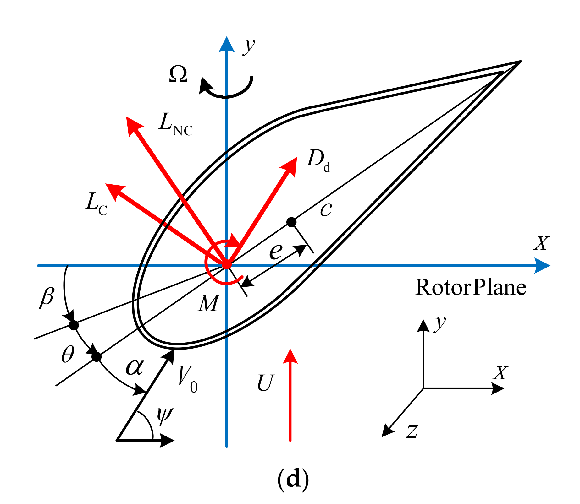
2.1. Structural Modelling and Aeroelastic System

Figure 1 shows a three-blade system driven by a slider-linkage mechanism implementing a unified pitch motion. Figure 1a is an auxiliary stereoscopic visual effect diagram, in which the slider-linkage mechanism is composed of a slider, screw rod and connecting rods. The right end of the screw rod is provided with a transmission gear which is driven by a stepping motor. The stepping motor drives the gear to drive the screw rod to rotate, to make the slider move forward or backward along the screw rod. The connecting rod structures are comprised of a fixed connecting rod fixed at one end and a sliding connecting rod movable at both ends. The distance from the position of the connecting rod fixedly connected with the blade (CRFCB), to the center of the root of the blade is described by R. When the slider moves back and forth, the connecting rods drive the blades to rotate around the centers of the blade roots, to realize the unified pitch movement. Figure 1b shows the half profile structure, showing the single airfoil section (per unit spanwise length) position r and the external wind speed U. The equivalent slider mass matched with the single airfoil section is M_b. Figure 1c shows the displacement h of the slider and the corresponding pitch angle β. The inertia of the section is modelled by the mass ρ_b, and the rotational inertia per unit of spanwise length is I_CG.

In view of the simplicity and rapidity of the aeroelastic performance analysis of 2D airfoil, typical section analysis is of a positive significance in the aeroelastic performance analysis of wind turbine blades or helicopter blades. In the present study, the typical, critical section of a large wind turbine blade is considered. The airfoil section, at the critical position r, is taken as the research object. Figure 1d shows the sectional coordinate system, the geometric parameters, motion parameters, and aerodynamic forces. The sectional structure is described in such a way that its motions have four independent translational degrees of freedom: an edgewise direction (lead-lag), denoted x; one perpendicular to that (flap-wise direction), denoted y; another elastic twist angle, denoted θ; and the external pitch angle β. The stall-induced aerodynamic forces are denoted by lift forces L_C (cyclic term) and L_NC (acyclic term), the drag force, $D_{\mathrm{d}}$, and the moment M = M_C + M_NC; herein, M_C is a cyclic torque, and M_NC is a non-cyclic torque. The wind velocity is denoted by U, with the relative wind angle denoted by ψ. The distance between the aeroelastic axis center and the center of gravity is e, and it is assumed that the aerodynamic forces act directly on the aeroelastic axis center. The rotating velocity of the blade section is denoted by Ω. The attack angle is α = ψ – β − θ; the inflow wind speed related to the relative wind angle ψ, can be expressed as $V_0=\sqrt{{\left(\mathsf{\Omega }r\right)}^2+U^2}$. The sectional parameters and related parameters are listed in

Table 1. The blade sectional parameters and related parameters.

Symbol	Quantity	Values
ωx	Angular frequency	18 rad s−1
ωy	Angular frequency	12 rad s−1
ωθ	Angular frequency	5π rad s−1
ρb	Mass per length of blade	50 kg m−1
ICG	Rotational inertia	10 m kg
U	Wind speed	5 m s−1
a	The sum of the lengths of the two connecting rods	2 m
ξx	Damping ratio	0.08
ξy	Damping ratio	0.06
ξθ	Damping ratio	0.06
e	Distance between the two centers	0.1 m
Ω	Angular frequency	0.6283 rad s−1
Mb	Equivalent slider mass	120 kg
R	Distance from CRFCB to the center of the blade root	0.8 m

.

Based on analysis of Lagrange’s equations, the model of bending/bending/twist vibrations for analyzing the effects of aerodynamic load control can be obtained. The equations are expressed in {y, x, θ, h, β} co-ordinates. The kinetic energy, T, and the potential energy, V, for the system are deduced as:

$$\begin{gathered} T=\frac{1}{2}{I}_{CG}{\left(\dot{\theta }+\dot{\beta }\right)}^2+\frac{1}{2}{\mathrm{M}}_{\mathrm{b}}{\dot{h}}^2+\frac{1}{2}{\rho }_{\mathrm{b}}{\left[\dot{y}\cos \left(\beta \right)+\dot{x}\sin \left(\beta \right)+e\left(\dot{\theta }+\dot{\beta }\right)\sin \left(\theta +\beta \right)+ \\ \dot{\beta }\left(x\cos \left(\beta \right)-y\sin \left(\beta \right)\right)+\dot{h}\right]}^2+\frac{1}{2}{\rho }_{\mathrm{b}}{[\dot{x}\cos \left(\beta \right)-\dot{y}\sin \left(\beta \right)-e\left(\dot{\theta }+\dot{\beta }\right)\cos \left(\theta +\beta \right)- \\ \dot{\beta }\left(y\cos \left(\beta \right)+x\sin \left(\beta \right)\right)]}^2 \end{gathered}$$

(1)

$$V=\frac{1}{2}\left[{\omega }_y^2{\rho }_{\mathrm{b}}{y}^2+{\omega }_x^2{\rho }_{\mathrm{b}}{x}^2+{\omega }_{\theta }^2\left(I_{\mathrm{CG}}+e^2{\rho }_{\mathrm{b}}\right){\theta }^2\right]$$

(2)

By using Lagrange’s equations based on Equations (1) and (2), the equations of motions of the aeroelastic system are respectively described as:

$$\begin{gathered} \ddot{y}+2{\xi }_y{\omega }_y\dot{y}+{\omega }_y^{2}y+\ddot{h}\cos \left(\beta \right)+e\left(\ddot{\theta }+\ddot{\beta }\right)\sin \left(\theta \right)+e{\left(\dot{\theta }+\dot{\beta }\right)}^2\cos \left(\theta \right)-\ddot{\beta }x-2\dot{\beta }\dot{x}= \\ {\rho }_{\mathrm{b}}^{-1}[D\sin \left(\Psi \right)+L_{\mathrm{C}}\cos \left(\Psi \right)+L_{\mathrm{NC}}\cos \left(\theta +\beta \right)] \end{gathered}$$

(3)

$$\begin{gathered} \ddot{x}+2{\xi }_x{\omega }_x\dot{x}+{\omega }_x^{2}x-\ddot{h}\sin \left(\beta \right)-e\left(\ddot{\theta }+\ddot{\beta }\right)\cos \left(\theta \right)+e{\left(\dot{\theta }+\dot{\beta }\right)}^2\sin \left(\theta \right)+\ddot{\beta }y+2\dot{\beta }\dot{y}= \\ {\rho }_{\mathrm{b}}^{-1}[D\cos \left(\Psi \right)-L_{\mathrm{C}}\sin \left(\Psi \right)-L_{\mathrm{NC}}\sin \left(\theta +\beta \right)] \end{gathered}$$

(4)

$$\begin{gathered} \ddot{\theta }+2{\xi }_{\theta }{\omega }_{\theta }\dot{\theta }+{\omega }_{\theta }^2\theta +\ddot{\beta }+\ddot{h}{r}_{\mathrm{E}}^{-2}\sin \left(\theta +\beta \right)+{\left[\left(I_{\mathrm{CG}}+e^2{\rho }_{\mathrm{b}}\right)/\left(I_{\mathrm{CG}}{\rho }_{\mathrm{b}}\right)\right]}^{-1}\left[\left(\ddot{y}\sin \left(\theta \right)- \\ \ddot{x}\cos \left(\theta \right)\right)+{\dot{\beta }}^2\left(x\cos \left(\theta \right)-y\sin \left(\theta \right)\right)+\ddot{\beta }\left(x\sin \left(\theta \right)+y\cos \left(\theta \right)\right)\right]=1/\left(I_{\mathrm{CG}}+e^2{\rho }_{\mathrm{b}}\right)M= \\ 1/\left(I_{\mathrm{CG}}+e^2{\rho }_{\mathrm{b}}\right)\left[M_{\mathrm{C}}+M_{\mathrm{NC}}\right] \end{gathered}$$

(5)

$${\mathrm{M}}_{\mathrm{b}}\ddot{h}-{\rho }_{\mathrm{b}}\left(2{\xi }_y{\omega }_y\dot{y}+{\omega }_y^{2}y\right)\cos \left(\beta \right)+{\rho }_{\mathrm{b}}(2{\xi }_x{\omega }_x\dot{x}-{\omega }_x^{2}x)\sin \left(\beta \right)=F$$

(6)

where F is the driving force of the slider to the connecting rod in pitch control, Equation (6). In the present study, F is separated from the aeroelastic system and will be used as an element in the subsequent, external control input T.

The pitch angle β is given by the external force F, from the angles of geometry of the slider-linkage mechanism motions, according to the actual design in the present study (see Appendix A), the mathematical relationship between pitch angle β and slider displacement h can be approximately described as:

$$h^2-h\left\{2a+4R\cos \left[\frac{1}{2}\left(\frac{\pi }{2}-\beta \right)\right]\sin \left(\frac{\beta }{2}\right)\right\}=4aR\cos \left[\frac{1}{2}\left(\frac{\pi }{2}-\beta \right)\right]\sin \left(\frac{\beta }{2}\right)-{\left[2R\sin \left(\frac{\beta }{2}\right)\right]}^2$$

(7)

2.2. Stall-Induced Nonlinear Aerodynamics Model

The nonlinear stall aerodynamics are included by use of the ONERA aerodynamics equations [13] to investigate the nonlinear, large amplitude, aeroelastic behaviors of hingeless composite rotor blades during hovering flight, that can develop into flutter oscillations. Considering the effect of a vertical wind direction and external pitch driving, it is assumed that the wind turbine’s rotor is in the state of uniform-speed rotation under the action of intelligent pitch control, and we rewrite the ONERA model as the ISNO aerodynamic model, in which the nonlinear parts of aerodynamic coefficients are fitted as a combination of 5-order polynomials and 8-order Taylor series. Aerodynamic forces (L_C, L_NC, D) and aerodynamic moments (M_C, M_NC) can be expressed as.

$$L_{\mathrm{C}}=\frac{1}{2}{\rho }_{\mathrm{a}}{S}_{\mathrm{L}}{V}_0\left(a_{0\mathrm{L}}{V}_0\Psi +{\Gamma }_{11\mathrm{L}}+{\Gamma }_{2\mathrm{L}}\right)$$

(8)

$$L_{\mathrm{NC}}=\frac{1}{2}{\rho }_{\mathrm{a}}{S}_{\mathrm{L}}\left[s_{\mathrm{L}}b\left(-1\right)V_0\cos \left(\alpha \right)\left(\dot{\beta }+\dot{\theta }\right)+l_{\mathrm{L}}b{V}_0\left(\dot{\theta }+\dot{\beta }+\mathsf{\Omega }\dot{y}\right)+k_{\mathrm{L}}{b}^2\left(\ddot{\theta }+\ddot{\beta }+\mathsf{\Omega }\ddot{y}\right)\right]$$

(9)

$$\begin{gathered} {\dot{\Gamma }}_{11\mathrm{L}}+{\lambda }_{\mathrm{L}}\frac{V_0}{b}{\Gamma }_{11\mathrm{L}}={\lambda }_{\mathrm{L}}{a}_{0\mathrm{L}}\frac{V_0}{b}{V}_0\sin \left(\alpha \right)+{\lambda }_{\mathrm{L}}{\sigma }_{\mathrm{L}}{V}_0\left(\dot{\theta }+\dot{\beta }+\mathsf{\Omega }\dot{y}\right)+{\gamma }_{\mathrm{L}}{a}_{0\mathrm{L}}\left(-V_0\cos \left(\alpha \right)\right)\left(\dot{\beta }+\dot{\theta }\right) \\ +{\gamma }_{\mathrm{L}}{\sigma }_{\mathrm{L}}b\left(\ddot{\theta }+\ddot{\beta }+\mathsf{\Omega }\ddot{y}\right) \end{gathered}$$

(10)

$${\ddot{\Gamma }}_{2\mathrm{L}}+a_{\mathrm{L}}\frac{V_0}{b}{\dot{\Gamma }}_{2\mathrm{L}}+r_{\mathrm{L}}{\left(\frac{V_0}{b}\right)}^2{\Gamma }_{2\mathrm{L}}=-r_{\mathrm{L}}\left[{\left(\frac{V_0}{b}\right)}^2{V}_0∆C_{\mathrm{L}}+e_{\mathrm{L}}\frac{V_0}{b}\left(V_0∆{\dot{C}}_{\mathrm{L}}\right)\right]$$

(11)

$$D_{\mathrm{d}}=\frac{1}{2}{\rho }_{\mathrm{a}}c{V}_0\left(V_0{C}_{\mathrm{D}0}+{\Gamma }_{\mathrm{D}2}\right)$$

(12)

$${\ddot{\Gamma }}_{\mathrm{D}2}+a_{\mathrm{D}}\frac{V_0}{b}{\dot{\Gamma }}_{\mathrm{D}2}+r_{\mathrm{D}}{\left(\frac{V_0}{b}\right)}^2{\Gamma }_{\mathrm{D}2}=-\left[r_{\mathrm{D}}{\left(\frac{V_0}{b}\right)}^2{V}_0∆C_{\mathrm{D}}+e_{\mathrm{D}}\frac{V_0}{b}{V}_0\cos \left(\alpha \right)\left(-\dot{\beta }-\dot{\theta }\right)\right]$$

(13)

$$M_{\mathrm{NC}}=\frac{1}{2}{\rho }_{\mathrm{a}}{S}_{\mathrm{M}}\left[s_{\mathrm{M}}b\left(-1\right)V_0\cos \left(\alpha \right)\left(\dot{\beta }+\dot{\theta }\right)+l_{\mathrm{M}}b{V}_0\left(\dot{\theta }+\dot{\beta }+\mathsf{\Omega }\dot{y}\right)+k_{\mathrm{M}}{b}^2\left(\ddot{\theta }+\ddot{\beta }+\mathsf{\Omega }\ddot{y}\right)\right]$$

(14)

$$M_{\mathrm{C}}=\frac{1}{2}{\rho }_{\mathrm{a}}{S}_{\mathrm{M}}{V}_0\left(a_{0\mathrm{M}}{V}_0\Psi +{\Gamma }_{11\mathrm{M}}+{\Gamma }_{2\mathrm{M}}\right)$$

(15)

$$\begin{gathered} {\dot{\Gamma }}_{11\mathrm{M}}+{\lambda }_{\mathrm{M}}\frac{V_0}{b}{\Gamma }_{11\mathrm{M}}={\lambda }_{\mathrm{M}}{a}_{0\mathrm{M}}\frac{V_0}{b}{V}_0\sin \left(\alpha \right)+{\lambda }_{\mathrm{M}}{\sigma }_{\mathrm{M}}{V}_0\left(\dot{\theta }+\dot{\beta }+\mathsf{\Omega }\dot{y}\right)+{\gamma }_{\mathrm{L}}{a}_{0\mathrm{M}}\left(-V_0\cos \left(\alpha \right)\right) \\ \left(\dot{\beta }+\dot{\theta }\right)+{\gamma }_{\mathrm{M}}{\sigma }_{\mathrm{M}}b\left(\ddot{\theta }+\ddot{\beta }+\mathsf{\Omega }\ddot{y}\right) \end{gathered}$$

(16)

$${\ddot{\Gamma }}_{2\mathrm{M}}+a_{\mathrm{M}}\frac{V_0}{b}{\dot{\Gamma }}_{2\mathrm{M}}+r_{\mathrm{M}}{\left(\frac{V_0}{b}\right)}^2{\Gamma }_{2\mathrm{M}}=-r_{\mathrm{M}}\left[{\left(\frac{V_0}{b}\right)}^2{V}_0∆C_{\mathrm{M}}+e_{\mathrm{M}}\frac{V_0}{b}\left(V_0∆{\dot{C}}_{\mathrm{M}}\right)\right]$$

(17)

where ρ_a is the air density, c is the chord length, with the half-chord length being b = c/2. If it is set to NACA0012 airfoil, other coefficients are as follows:

$S_{\mathrm{L}}=c$, $s_{\mathrm{L}}=\pi$, $l_{\mathrm{L}}=0$, $k_{\mathrm{L}}=0.5\pi$, $a_{0\mathrm{L}}={\sigma }_{\mathrm{L}}=5.9$, ${\lambda }_{\mathrm{L}}=0.15$, ${\gamma }_{\mathrm{L}}=0.55$, $a_{\mathrm{L}}=0.25+0.4{\left(∆C_{\mathrm{L}}\right)}^2$, $r_{\mathrm{L}}={\left[0.2+0.23{\left(∆C_{\mathrm{L}}\right)}^2\right]}^2$, $e_{\mathrm{L}}=-2.7{\left(∆C_{\mathrm{L}}\right)}^2$; $S_{\mathrm{M}}=c^2$, $s_{\mathrm{M}}=l_{\mathrm{M}}=-\pi /4$, $k_{\mathrm{M}}=-3\pi /16$, $a_{0\mathrm{M}}={\sigma }_{\mathrm{M}}={\lambda }_{\mathrm{M}}=r_{\mathrm{M}}=0$, $a_{\mathrm{M}}=a_{\mathrm{L}}$, $r_{\mathrm{M}}=r_{\mathrm{L}}$, $e_{\mathrm{M}}=e_{\mathrm{L}}$, $C_{\mathrm{D}0}=0.014$, $a_{\mathrm{D}}=0.32$, $r_{\mathrm{D}}={\left[0.2+0.1{\left(∆C_{\mathrm{L}}\right)}^2\right]}^2$, $e_{\mathrm{D}}=-0.015{\left(∆C_{\mathrm{L}}\right)}^2$.

In the present study, the nonlinear parts, ∆C_L and ∆C_M, in the above aerodynamic coefficients are fitted as a combination of 5-order rationales and 8-order Taylor series as follows:

$$∆C_{\mathrm{L}}=\left({\mathrm{p}}_1\times {\alpha }^5+{\mathrm{p}}_2\times {\alpha }^4+{\mathrm{p}}_3\times {\alpha }^3+{\mathrm{p}}_4\times {\alpha }^2+{\mathrm{p}}_5\times \alpha \right)/\left({\alpha }^4+{\mathrm{q}}_1\times {\alpha }^3+{\mathrm{q}}_2\times {\alpha }^2++{\mathrm{q}}_3\times \alpha +{\mathrm{q}}_4\right)$$

(18)

$$∆C_{\mathrm{M}}={\mathrm{a}}_0+{{\displaystyle \sum }}_{i=1}^8[{\mathrm{a}}_i\cos \left(w\alpha \right)+{\mathrm{b}}_i\sin \left(w\alpha \right)]$$

(19)

and the nonlinear parts ∆C_D can be accurately described as:

$$∆C_{\mathrm{D}}=-7.35\times {10}^4\alpha -4.5111\times {10}^{-5}{\alpha }^2-2.6384{\alpha }^3$$

(20)

where the related parameters in Equations (18) and (19) are listed in

Table 2. The related parameters in Equations (18) and (19).

Nonlinear Parts	Parameters	95 Percent Confidence Intervals
∆CL	p1 = −0.001329	% (−0.01969, 0.01704)
	p2 = −0.5626	% (−0.5976, −0.5276)
	p3 = 0.2003	% (0.1861, 0.2146)
	p4 = −0.02494	% (−0.02771, −0.02216)
	p5 = 0.001236	% (0.0009995, 0.001472)
	p6 = −1.86e−05	% (−2.571 × 10−5, −1.15 × 10−5)
	q1 = −0.4713	% (−0.4891, −0.4534)
	q2 = 0.09069	% (0.08319, 0.09819)
	q3 = −0.008524	% (−0.009628, −0.00742)
	q4 = 0.0003258	% (0.0002697, 0.0003818)
∆CM	a0 = 0.03932	% (0.03651, 0.04213)
	a1 = −0.0357	% (−0.04107, −0.03033)
	b1 = −0.02527	% (−0.02976, −0.02078)
	a2 = −0.01138	% (−0.01811, −0.004655)
	b2 = −0.03203	% (−0.03688, −0.02718)
	a3 = 0.009252	% (0.00298, 0.01552)
	b3 = −0.02015	% (−0.02402, −0.01629)
	a4 = 0.01412	% (0.01034, 0.01791)
	b4 = −0.0004783	% (−0.004383, 0.003427)
	a5 = 0.005038	% (0.0008763, 0.0092)
	b5 = 0.01216	% (0.008025, 0.01629)
	a6 = −0.006258	%(−0.01096, −0.001556)
	b6 = 0.0116	% (0.005918, 0.01729)
	a7 = −0.009751	% (−0.01324, −0.006259)
	b7 = 0.003518	% (−0.002786, 0.009821)
	a8 = −0.005128	% (−0.008551, −0.001705)
	b8 = −0.002258	% (−0.006777, 0.002261)
	w = 3.682	% (3.496, 3.867)

by using numerical expressions under MATLAB; herein, the 95 percent confidence interval is after the “%” sign. The lengths of the confidence intervals are generally small, which reflects the reliability of the data fitting method.

It should be noted that we adopt the method of fitting the nonlinear terms of aerodynamic forces here, which does not mean that the fitted aerodynamic forces data is more accurate than the original ONERA model data in reference [13], but in order to smoothly execute the subsequent iterative algorithm process for dealing with nonlinear systems. However, on the basis of enough fitting points, the 95% confidence intervals are narrow enough, which shows that the fitting method can effectively reflect the real values.

3. Amplitude Control Based on IILC

3.1. System Simplification

The ILC algorithm is often used to deal with the large-scale, time-domain responses of nonlinear systems; however, for multivariable systems, the iterative process will be very long. For the control system, which needs a fast response to restrain the flutter, especially for the actual hardware control system such as programmable logic controllers (PLCs) that are currently the controllers of most large wind turbines [15], it has lost practical significance and practical value because of the complexity of the most intelligent control algorithms, so this design in the present study, will further simplify the aeroelastic system.

Inspired by the flow visualization of a dynamic stall on a pitching airfoil in a wind tunnel [16], and the immediacy of the velocity distribution of the blade model considering horizontal wind [17], and the operation control of a high-speed train by using spatial ILC [18] as well, we might as well assume that the pitch control law is used to satisfy and match the ILC algorithm on the one hand, and make the pitch angle change with the elastic torsion angle at any time on the other hand. In this way, as long as the elastic torsion angle is generated, it will be eliminated by pitch motion, so that the elastic torsion displacement almost always fluctuates around “0”, then we can ignore the elastic torsion deformation θ in the aeroelastic system, so as to simplify the system. Not only the structural equations are simplified, but also the aerodynamics forces are simplified. For example, if the effect of the elastic twist θ is not considered, the aerodynamic torque M and its related terms can be ignored.

In addition, in view of the nonlinearity of the independent Formula (7), we can make the pitch system work at a certain equilibrium position. So, we can use a linearization method, based on the equilibrium position, to realize the linearization. The linearized equation of Formula (7) is h = 1.6β (see Appendix A). Taking h = 1.6β into Formula (6), the equivalent transformed pitch system equation can be obtained.

The simplified equations of motions can be described as:

$$\begin{gathered} \ddot{y}+2{\xi }_y{\omega }_y\dot{y}+{\omega }_y^{2}y+1.6\ddot{\beta }\cos \left(\beta \right)+e{\left(\dot{\beta }\right)}^2-\ddot{\beta }x-2\dot{\beta }\dot{x}={\rho }_{\mathrm{b}}^{-1}[D\sin \left(\Psi \right)+ \\ {L}_{\mathrm{C}}\cos \left(\Psi \right)+L_{\mathrm{NC}}\cos \left(\beta \right)] \end{gathered}$$

(21)

$$\begin{gathered} \ddot{x}+2{\xi }_x{\omega }_x\dot{x}+{\omega }_x^{2}x-1.6\ddot{\beta }\sin \left(\beta \right)-e\ddot{\beta }+\ddot{\beta }y+2\dot{\beta }\dot{y}={\rho }_{\mathrm{b}}^{-1}[D\cos \left(\Psi \right)- \\ {L}_{\mathrm{C}}\sin \left(\Psi \right)-L_{\mathrm{NC}}\sin \left(\beta \right)] \end{gathered}$$

(22)

$$1.6{\mathrm{M}}_{\mathrm{b}}\ddot{\beta }-{\rho }_{\mathrm{b}}\left(2{\xi }_y{\omega }_y\dot{y}+{\omega }_y^{2}y\right)\cos \left(\beta \right)+{\rho }_{\mathrm{b}}(2{\xi }_x{\omega }_x\dot{x}-{\omega }_x^{2}x)\sin \left(\beta \right)=F$$

(23)

with aerodynamics expressions described as follows:

$$L_{\mathrm{C}}=\frac{1}{2}{\rho }_{\mathrm{a}}{S}_{\mathrm{L}}{V}_0\left(a_{0\mathrm{L}}{V}_0\Psi +{\Gamma }_{11\mathrm{L}}+{\Gamma }_{2\mathrm{L}}\right)$$

(24)

$$L_{\mathrm{NC}}=\frac{1}{2}{\rho }_{\mathrm{a}}{S}_{\mathrm{L}}\left[s_{\mathrm{L}}b\left(-1\right)V_0\cos \left(\alpha \right)\dot{\beta }+l_{\mathrm{L}}b{V}_0\left(\dot{\beta }+\mathsf{\Omega }\dot{y}\right)+k_{\mathrm{L}}{b}^2\left(\ddot{\beta }+\mathsf{\Omega }\ddot{y}\right)\right]$$

(25)

$$\begin{gathered} {\dot{\Gamma }}_{11\mathrm{L}}+{\lambda }_{\mathrm{L}}\frac{V_0}{b}{\Gamma }_{11\mathrm{L}}={\lambda }_{\mathrm{L}}{a}_{0\mathrm{L}}\frac{V_0}{b}{V}_0\sin \left(\alpha \right)+{\lambda }_{\mathrm{L}}{\sigma }_{\mathrm{L}}{V}_0\left(\dot{\beta }+\mathsf{\Omega }\dot{y}\right)+{\gamma }_{\mathrm{L}}{a}_{0\mathrm{L}}\left(-V_0\cos \left(\alpha \right)\right)\dot{\beta }+ \\ {\gamma }_{\mathrm{L}}{\sigma }_{\mathrm{L}}b\left(\ddot{\beta }+\mathsf{\Omega }\ddot{y}\right) \end{gathered}$$

(26)

$${\ddot{\Gamma }}_{2\mathrm{L}}+a_{\mathrm{L}}\frac{V_0}{b}{\dot{\Gamma }}_{2\mathrm{L}}+r_{\mathrm{L}}{\left(\frac{V_0}{b}\right)}^2{\Gamma }_{2\mathrm{L}}=-r_{\mathrm{L}}\left[{\left(\frac{V_0}{b}\right)}^2{V}_0∆C_{\mathrm{L}}+e_{\mathrm{L}}\frac{V_0}{b}\left(V_0∆{\dot{C}}_{\mathrm{L}}\right)\right]$$

(27)

$$D_{\mathrm{d}}=\frac{1}{2}{\rho }_{\mathrm{a}}c{V}_0\left(V_0{C}_{\mathrm{D}0}+{\Gamma }_{\mathrm{D}2}\right)$$

(28)

$${\ddot{\Gamma }}_{\mathrm{D}2}+a_{\mathrm{D}}\frac{V_0}{b}{\dot{\Gamma }}_{\mathrm{D}2}+r_{\mathrm{D}}{\left(\frac{V_0}{b}\right)}^2{\Gamma }_{\mathrm{D}2}=-\left[r_{\mathrm{D}}{\left(\frac{V_0}{b}\right)}^2{V}_0∆C_{\mathrm{D}}+e_{\mathrm{D}}\frac{V_0}{b}{V}_0\cos \left(\alpha \right)\left(-\dot{\beta }\right)\right]$$

(29)

In addition, the attack angle in the nonlinear parts, ∆C_L, ∆C_M and ∆C_D of Equations (18)–(20), can be expressed as α = ψ − β.

Assuming that the state variables vector is q(t) = [y, x, β, Γ_11L, Γ_2L, Γ_D2]^T, considering in conjunction with Formulas (21)–(29), we can get the simplified aeroelastic system:

$${\left.D\left(q\right)\right|}_{6\times 6}\ddot{q}+{\left.C\left(q,\dot{q}\right)\right|}_{6\times 6}\dot{q}+G{\left.\left(q,\dot{q}\right)\right|}_{6\times 1}+{\left.T_{\mathrm{a}}\right|}_{6\times 1}={\left.T\right|}_{6\times 1}$$

(30)

where D is the inertial term; C is the damping term; G is the combination of the variable parts of the structural terms and aerodynamic terms; T_a is constant parts in the aerodynamic terms, and variable parts only changing with wind speed. T is the external control input.

3.2. An Improved ILC (IILC) Algorithm Based on Residual Effect

An ILC algorithm is suitable for a controlled object with repetitive motion. It depends on the precise mathematical model of the system, and can deal with the nonlinear, strong coupling dynamic system [14]. The IILC algorithm used here is to add a robust term to its control law and consider the linearized residual effect to realize adaptive iterative control. It does not depend on the precise mathematical model of the system, and can deal with the nonlinear, strong coupling dynamic system with “very high uncertainty”. This “uncertainty” often comes from the aerodynamic uncertainty under stall-induced vibration, due to the fact that the aerodynamic model itself is only an experimental qualitative description. Therefore, the algorithm based on residual effect analysis adopted in the present study can deal with the uncertainty of the aeroelastic system model as much as possible.

The controller design process is as follows.

Along the instruction trajectory $\left(q_{\mathrm{d}}\left(t\right),{\dot{q}}_{\mathrm{d}}\left(t\right),{\ddot{q}}_{\mathrm{d}}\left(t\right)\right)$, assuming that the error is $et=q_{\mathrm{d}}t-qt$, we adopt the Taylor formula based on the first-order expansion, then the Equation (30) can be linearized to:

$$D\ddot{e}+\left(C+C_1\right)\dot{e}+Qe+n\left(\ddot{e},\dot{e},e,t\right)-T_a=H-T$$

(31)

where

$$C_1={\left.\frac{\partial C}{\partial \dot{q}}\right|}_{q_{\mathrm{d}},{\dot{q}}_{\mathrm{d}}}{\dot{q}}_{\mathrm{d}}\left(t\right)+{\left.\frac{\partial G}{\partial \dot{q}}\right|}_{q_{\mathrm{d}},{\dot{q}}_{\mathrm{d}}}, Q={\left.\frac{\partial D}{\partial \dot{q}}\right|}_{q_{\mathrm{d}}}{\ddot{q}}_{\mathrm{d}}\left(t\right)+{\left.\frac{\partial G}{\partial \dot{q}}\right|}_{q_{\mathrm{d}},{\dot{q}}_{\mathrm{d}}}+{\left.\frac{\partial C}{\partial q}\right|}_{q_{\mathrm{d}},{\dot{q}}_{\mathrm{d}}}{\dot{q}}_{\mathrm{d}}\left(t\right)+{\left.\frac{\partial G}{\partial \dot{q}}\right|}_{q_{\mathrm{d}}},$$

$$H=D\left({\dot{q}}_{\mathrm{d}}\left(t\right)\right){\ddot{q}}_{\mathrm{d}}\left(t\right)+C\left(q_{\mathrm{d}}\left(t\right),{\dot{q}}_{\mathrm{d}}\left(t\right)\right){\dot{q}}_{\mathrm{d}}\left(t\right)+G\left(q_{\mathrm{d}}\left(t\right)\right),$$

$$n\left(\ddot{e},\dot{e},e,t\right)=-{\left.\frac{\partial D}{\partial q}\right|}_{q_{\mathrm{d}}}\ddot{e}\dot{e}-{\left.\frac{\partial C}{\partial q}\right|}_{q_{\mathrm{d}},{\dot{q}}_{\mathrm{d}}}\dot{e}e-{\left.\frac{\partial C}{\partial q}\right|}_{q_{\mathrm{d}},{\dot{q}}_{\mathrm{d}}}{\left(\dot{e}\right)}^2+O_D\left(·\right)\ddot{q}+O_C\left(·\right)\dot{q}-O_G\left(·\right);$$

herein, O_D, O_C, O_G are the residual terms of D, C, G after performing first-order expansion, respectively.

In order to perform the iterative process, we rewrite Formula (31) into a dynamic equation based on the number of iterations $j$, then we can get the expressions of the j-th and (j + 1)-th iterations:

$$\left\{\begin{array}{c}D{\ddot{e}}^j+\left(C+C_1\right){\dot{e}}^j+Q{e}^j+n\left({\ddot{e}}^j,{\dot{e}}^j,e^j,t\right)-T_a=H-T^j\\ D{\ddot{e}}^{j+1}+\left(C+C_1\right){\dot{e}}^{j+1}+Q{e}^{j+1}+n\left({\ddot{e}}^{j+1},{\dot{e}}^{j+1},e^{j+1},t\right)-T_a=H-T^{j+1}\end{array}\right.$$

(32)

The robust iterative learning control law can be designed as:

$$T^j\left(t\right)=K_{\mathrm{P}}^j{e}^j\left(t\right)+K_{\mathrm{D}}^j{\dot{e}}^j\left(t\right)+T^{j-1}\left(t\right)+E\mathrm{sgn}\left[{\dot{e}}^{j-1}\left(t\right)+e^{j-1}\left(t\right)\right]$$

(33)

where E is the control parameter with its value greater than zero, which satisfy

$$\Vert d^{j+1}\left(t\right)\Vert -d^j\left(t\right)\le E;$$

(34)

herein, $d^j\left(t\right)=-n\left({\ddot{e}}^j,{\dot{e}}^j,e^j,t\right)+T_{\mathrm{a}}$.

In this design, the moderate parameters can be taken as:

$$E=1;K_{\mathrm{P}}^0=K_{\mathrm{D}}^0=K_0\times I_E,K_{\mathrm{P}}^j=K_{\mathrm{D}}^j=2j{K}_{\mathrm{P}}^0,j=1,2,\cdots ,N$$

(35)

where I_E is identity matrix I_6×6; K₀ is the control gain that can be obtained by another adaptive tuning in the iterative process by a PID controller by using a single neuron proportional–derivative (SNPD) control with an improved Hebb learning algorithm [19]. In Equation (33), $E$ is an integer greater than zero. Generally speaking, it affects the average value of fluctuation, but does not affect the amplitude of fluctuation, so we normalize it. We let ‘$K_{\mathrm{P}}^0=K_{\mathrm{D}}^0$’, which is to reduce the amount of computation of the computer and improve the operation speed. ‘$K_{\mathrm{D}}^j=2j{K}_{\mathrm{P}}^0$’ is an empirical setting.

For the controlled error object $e^j$ in Equation (33), i.e.,

$${\tau }_{\mathrm{pd}}^j={\tau }_{\mathrm{pd}}\left(j\right)=K_{\mathrm{P}}^j{e}^j+K_{\mathrm{D}}^j{\dot{e}}^j=K_{\mathrm{P}}\left(j\right)e\left(j\right)+K_{\mathrm{D}}\left(j\right)\dot{e}\left(j\right).$$

(36)

Figure 2 shows the flow chart of applications of the SNPD algorithm. Herein, the calculus module calculates two quantities:

$$\left\{\begin{array}{c}{v}_1\left(j\right)=e\left(j\right) \\ v_2\left(j\right)={∆}^{2}e\left(j\right)=e\left(j\right)-2e\left(j-1\right)+e\left(j-2\right)\end{array}\right.$$

(37)

The update rules of the two weights can be written as:

$$\left\{\begin{array}{c}{w}_1\left(j\right)=w_1\left(j-1\right)+{\eta }_{\mathrm{p}}e\left(j\right){\tau }_{pd}\left(j\right)\left[e\left(j\right)-∆e\left(j\right)\right]\\ w_2\left(j\right)=w_2\left(j-1\right)+{\eta }_{\mathrm{d}}e\left(j\right){\tau }_{pd}\left(j\right)\left[e\left(j\right)-∆e\left(j\right)\right]\end{array}\right.$$

(38)

where η_p, η_d are adaptive proportional and derivative learning rates, respectively. The two weights are state variables, hence the SNPD control law is:

$${\tau }_{\mathrm{pd}}\left(j\right)={\tau }_{\mathrm{pd}}\left(j-1\right)+K{{\displaystyle \sum }}_{i=1}^2\left[w_i\left(j\right)v_1\left(j\right)/{{\displaystyle \sum }}_{i=1}^2\left|w_i\left(j\right)\right|\right]$$

(39)

Since the neuron node is capable of learning highly nonlinear dynamics in aerodynamic modeling [20], the adaptive adjustment process of K_P and K_D in the IILC control law Formula (33) is a complete proportional–derivative (PD) control process, and there are built-in PD controllers in PLCs’ hardware, the IILC algorithm is more suitable for its engineering application in PLCs by using OPC technology [15] to connect the neural network theory in a PC and SNPD controller in PLC, which is also another advantage of the present design.

The consistency of vibration tracking and amplitude control can be described from the change of the amplitudes of the preset trajectories. On the one hand, if the amplitude of the preset trajectory is moderate, when the trajectory tracking is realized, the vibration amplitude of the blade is actually in a reasonable vibration range. On the other hand, if the amplitude of the preset trajectory is small enough, when the trajectory tracking is completed, we might achieve the absolutely convergent control effect of blade displacement, that is, the purpose of amplitude stability of a nonlinear system.

4. Results and Discussions

To investigate the trajectory tracking of the airfoil section at position r by using the IILC algorithm mentioned above, some cases intended to highlight the effect of amplitude control will be presented. The related parameters of airfoil, including structural parameters and external motion parameters, are described in Table 1. According to practical experience, in a stall-induced state, the dangerous section of the wind turbine blade is often located at the position of 1/4 to 1/3 of the span from the blade root. For the blade with a span of about 10 m, we might as well take the airfoil section position at r = 2.5 m, with the maximum chord length being c = 1.5 m. For the six variables in Equation (30) that need to be controlled, we might as well assume that the desired trajectories are:

$$q_{1\mathrm{d}}\left(t\right)=q_{3\mathrm{d}}\left(t\right)=q_{5\mathrm{d}}\left(t\right)=0.2\sin \left(3t\right);q_{2\mathrm{d}}\left(t\right)=q_{4\mathrm{d}}\left(t\right)=q_{6\mathrm{d}}\left(t\right)=0.2\cos \left(3t\right)$$

(40)

Equation (40) is the set tracking target. We chose the sine function as the target. The value A_m = 0.2 is the amplitude value of sinusoidal signal. The smaller the amplitude value of the sinusoidal signal, the higher the accuracy requirements for the control algorithm. This is because when the tracking result is realized, the controlled physical quantity has actually been limited to ±0.2, which actually achieves the purpose of amplitude control, compared with the uncontrolled state. The value Ω₀ = 3 is the frequency of the sinusoidal signal. The smaller the frequency, when the controlled displacement tends to be stable, the higher the performance requirements of the control algorithm. For the blade tip response of the wind turbine, when the controlled system tends to be stable, the smaller the vibration frequency Ω₀, the better the system performance. In practical application, Ω₀ = 3 is an acceptable fluctuation frequency.

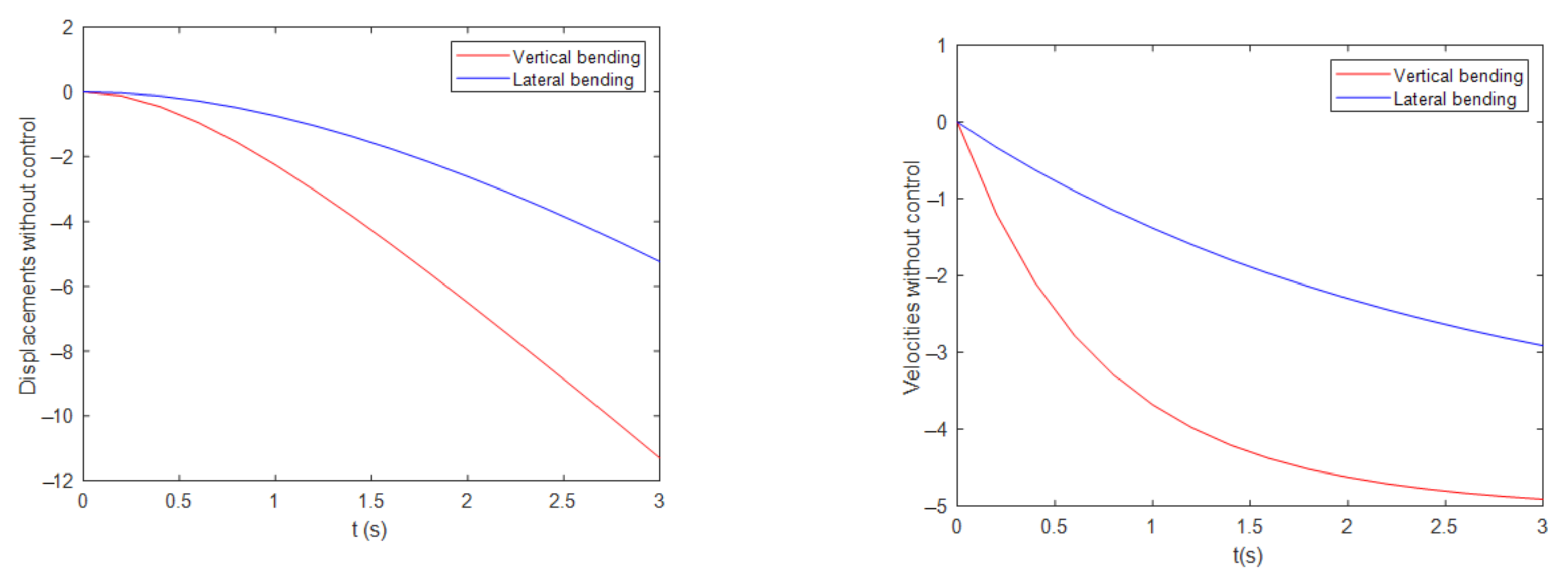
4.1. Absolutely Divergent Instability

Figure 3 shows the uncontrolled blade sectional time responses of the vertical bending displacement y in a flap-wise direction, and the lateral bending x in a lead-lag direction, and related velocities’ responses, respectively, with wind speed U = 5 ms⁻¹. All the two motions are in states of rapid divergences. Especially for the displacements, both vertical bending y and lateral bending x are rapidly divergent and more than the sectional position length of r = 2.5 m within the 0.5 s time. This is precisely the absolutely divergent instability: assuming that if the blade span is large enough, the size of all diverging shifts over time will be incredible.

Therefore, vibration control is necessary. The amplitude control method mentioned above can just meet the goal of vibration control.

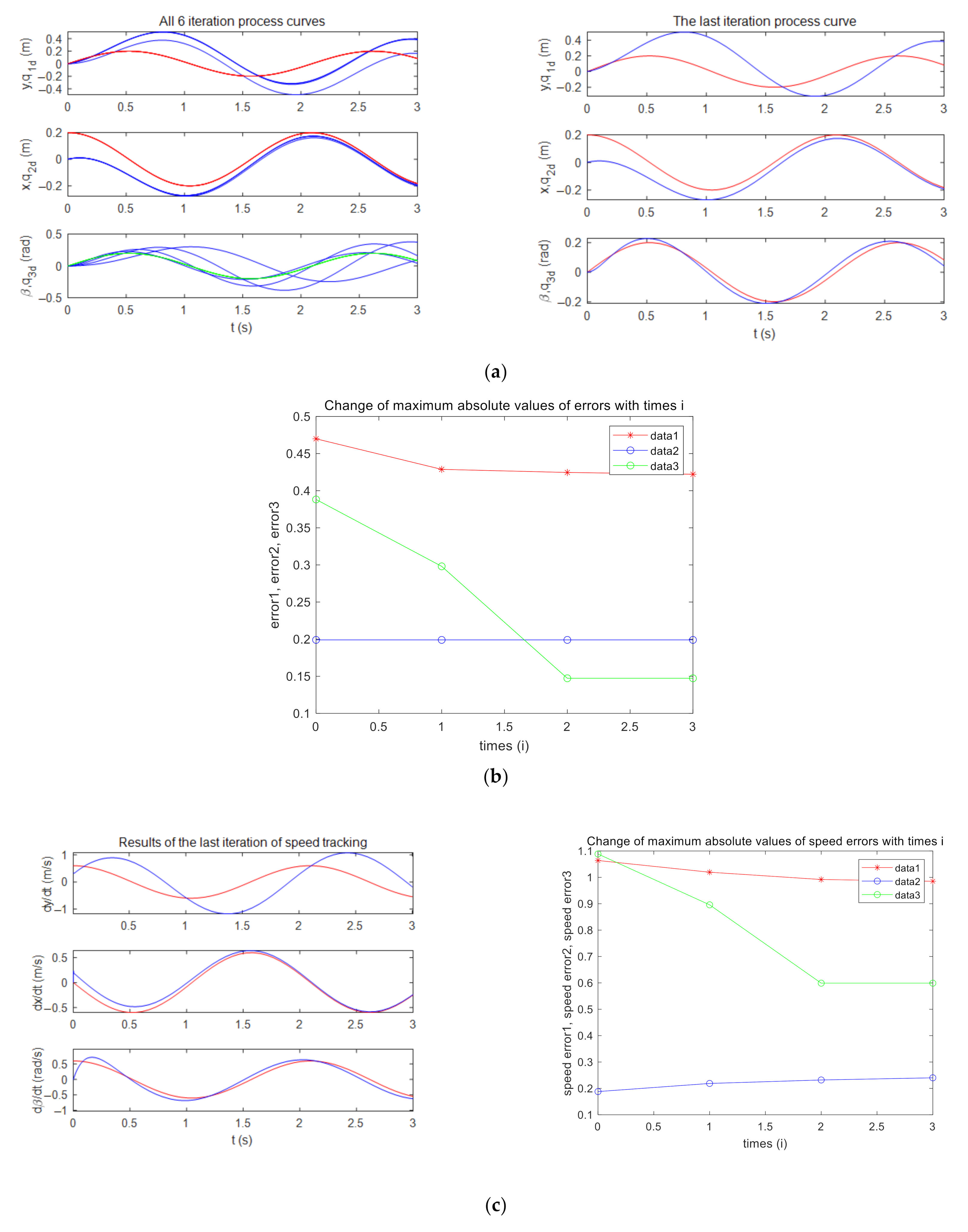
4.2. Realization of Amplitude Control by Using IILC Algorithm

Due to the difficulty of the iterative operation and the complexity of the operation process, in order to reduce the total iteration operation, the number of iterations is set to 6, with the total iteration time being 3 s. Figure 4a shows the variable fluctuations of all six iterations (note that the curves in several fluctuations coincide) and the variable fluctuations of the last iteration within 3 s. The preset trajectories are q_jd (j = 1,2,3), which are denoted by red or green curves. The variable fluctuations of the vertical bending displacements y, lateral bending displacements x, and pitch angles β are denoted by blue curves. The amplitudes of the vertical bending displacements in the six iterations are limited to a range of ±0.6 m, with those of the lateral bending displacements limited to almost ±0.2 m. Compared with the divergent instability displacements in Figure 2, the fluctuation amplitudes illustrated in Figure 4a shows the fluctuation in a limited interval and achieves the purpose of amplitude control. Of course, if you set a larger number of iterations and a longer iteration execution time, the tracking effect will be more obvious, and the fluctuation range may be limited to a smaller range. From the fluctuation process of pitch angle, it tracks the set value well, and is basically within the range of ±0.2 rad, that is, the angle range of ±11.5 degrees. This is a numerical range that is physically easy to be realized, and there will be no physical interference in the physical process of pitch motion.

Figure 4b shows the maximum absolute values of errors j(j = 1,2,3) of variable fluctuations in the three iterations. Abscissa is the number of iterations, times (i), which is limited to i = 3. After three iterations, the errors are basically at constant values, which reflects good tracking effects.

Figure 4c shows the speed fluctuations of the last iteration and the maximum speed errors during the three iterations, which shows an effect almost similar to the fluctuations of the displacements and errors, and reflects the good tracking effects in the implementation of the IILC algorithm.

Figure 4d shows the force fluctuation of the slider thrust F, which is the driving force from the pitch motion of the stepping motor. Its fluctuation is stable and attenuated as time goes on, which means that, with the coincidence of the tracking effect, the driving force tends to converge, which inevitably means that the pitch angle will eventually converge and stabilize with the passage of time, reflecting the feasibility of the realization process of blade flutter suppression.

4.3. Algorithm Requirements for Residual Effect

The effectiveness of the IILC algorithm is based on residual analysis, so the validity of the residual range itself must be guaranteed in the calculation process. The effectiveness of the tracking process of displacements and velocities shown in Figure 4 has implied the effectiveness of the residual calculation range of each variable during the implementation of the IILC algorithm. However, the nonlinear terms in Equations (18) and (19) in the aerodynamic coefficients adopt the method of fitting data, hence the effectiveness of the residual analysis of the fitting process should also be tested.

For the nonlinear terms, ∆C_L and ∆C_M, Figure 5 vividly illustrates the original data points, fitting curves and residual analysis in the fitting process, calculated by using the Residual Analyzer (Note that “\DeltaC_L“ refers to ∆C_L, “\DeltaC_M“ refers to ∆C_M and “\alpha“ refers to α). The residual diagrams take the independent variables α as the abscissa values, and the residuals as the ordinate values. The depicted points fluctuate up and down around the straight line with the residual equal to zero, and the absolute values of the residuals are relatively small, indicating that the fitted curves have good fitting performances for the original data points.

When α changes in the range of 0~π/2, whether it is for the residuals of ∆C_L or the residuals of ∆C_M, all residual data points are basically in the range of ±0.06, and only a few residual points exceed the range of ±0.05, reflecting the effectiveness of the data fitting process and the accuracy of the estimation. Of course, it needs to be emphasized again that the fitted curve itself is not more accurate than the original data points, but on the basis of meeting the requirements of the fitting error and the residual effect, the smoothed, continuous and nonlinear terms described by mathematical expressions can be directly applied to the iterative algorithm, so that the automation of the iterative process can be realized.

4.4. Robustness of the IILC Algorithm

In abnormal and dangerous situations, the effectiveness of the control algorithm is often the key to blade safety. Therefore, the robustness of the IILC algorithm is very important. Since wind velocity acting on wind wheel does not exceed 10 m s⁻¹ on most land areas where the turbulence intensity data change less, and the surface fluctuation trend is relatively stable [21], therefore, another case, intended to highlight the effect of the IILC method under the condition of a wind speed U = 10 ms⁻¹, is presented below, with time responses analysis and tracking results demonstrated.

Figure 6 illustrates the uncontrolled time responses with U = 10 ms⁻¹ (a), and the variable fluctuations of all the three iterations during the tracking process (b). Figure 6a obviously shows a greater degree of divergent instability compared with that in Figure 3. Figure 6b shows the variable fluctuations of all the three iterations during the tracking process. With the increase of divergence instability, the complexity of the iterative process increases, so we only tested the iterative process three times. However, the results show that the amplitudes of time responses are well controlled in the three iterations, which further reflects the reliability and robustness of the proposed IILC iterative algorithm. In particular, it is noted that the fluctuations of pitch angle are limited to the range of ±0.5 rad, i.e., ±28.7°, which is still completely within the physically achievable range.

In addition, since soft in-plane rotating blades may have different types of vibration modes with lesser degrees of lead-lag/twist couplings, different nonlinear trends may be expected of rotating blades. This study provides methodologies for directly dealing with nonlinear aeroelastic problems of pitching blades. However, all of the simulation results demonstrated in the present study are likely related to hingeless hard in-plane rotor blades and should qualitatively represent the nonlinear characteristics of blades with large-amplitude vibration.

In terms of external pitch motion, the developed model is not only suitable for the unified pitching blade proposed in this study, but also for the independent pitching blade and, furthermore, for the analysis of the stall state with large divergent unstable displacements at the blade tip. The stall model with fitted coefficients can be used to solve not only the light stall nonlinear system, but also the deep stall nonlinear system.

5. Conclusions

The stall-induced nonlinear aeroelastic behavior and amplitude control of the blade section are investigated. Some concluding remarks can be drawn from the numerical simulation illustrations:

• The nonlinear aeroelastic system equations are deduced. The nonlinear ISNO aerodynamic model is applied, with the nonlinear items in the ONERA model, fitted to be applied in the iterative algorithm. The validity of the residuals in the process of data fitting and the validity of the residuals in the process of the iterative algorithm operation have been tested directly or indirectly, respectively.
• The amplitude control of the wind turbine blade, based on unified pitch motion driven by a slider-linkage mechanism, is investigated by using the IILC algorithm that focuses on residual analysis and residual effect.
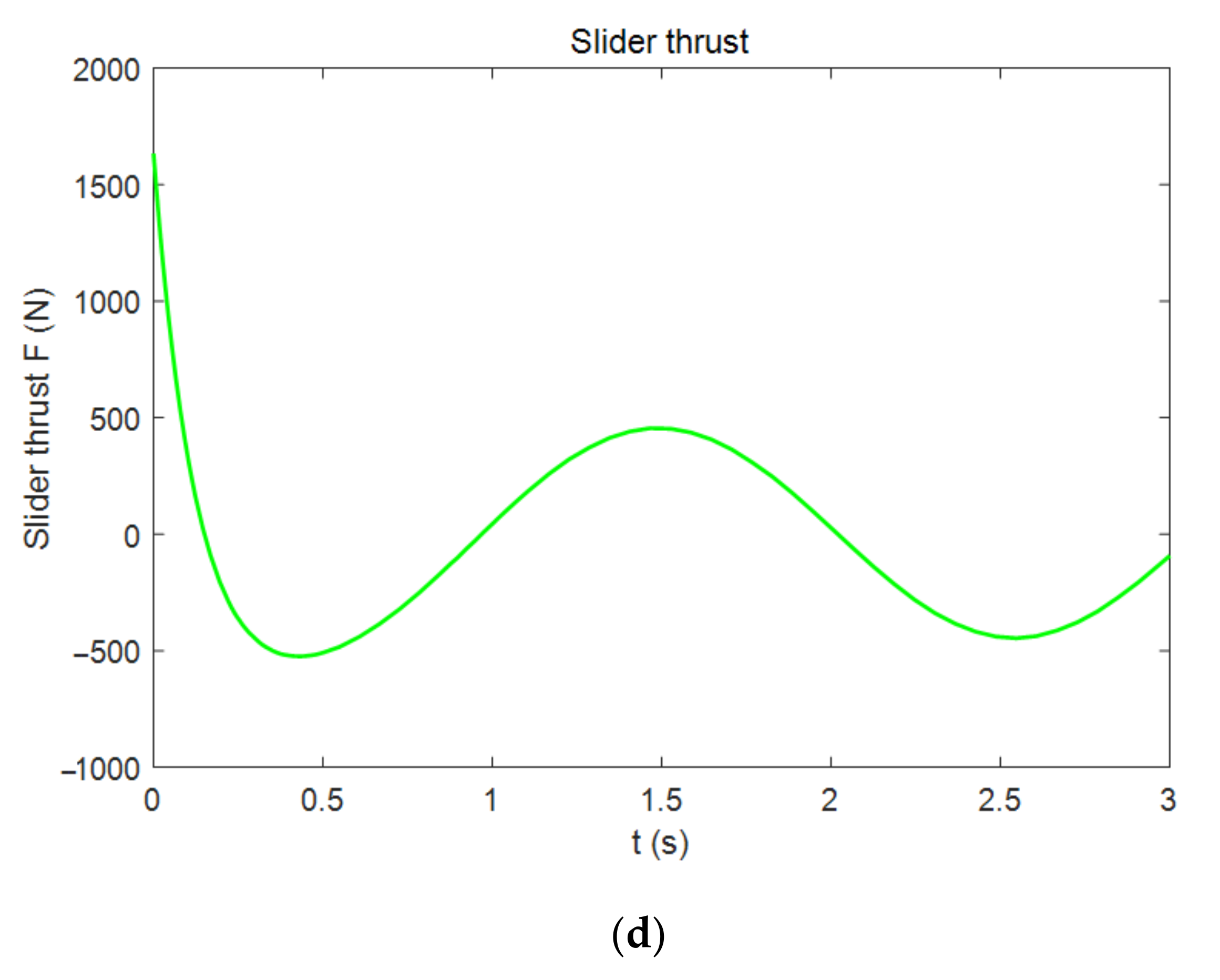
• The slider-linkage mechanism is driven by screw pod transmission. The rotation of the screw rod is driven by the stepping motor. The stability of the stepping motor movement and the maturity of real-time control are more conducive to the engineering application of the step-by-step operation of the iterative algorithm.
• Time responses of displacements and velocities, and trajectory tracking results based on the IILC algorithm are investigated. Good tracking results show the effectiveness of the IILC algorithm. Numerical simulations based on different parameters prove that the algorithm is superior in reliability and robustness.
• There are two keys to the implementation of the IILC algorithm. First, the method of fitting aerodynamic coefficients is necessary, which is the key to the smooth operation of the IILC algorithm; secondly, the simplification of the aeroelastic system is also necessary, which is the key to accelerating the IILC algorithm, so as to facilitate the engineering application of the algorithm.
• As for further development, additional study needs to be performed on different types of blades, with more realistic blade specifications and more reliable dynamic stall characteristics. Further research on stall states should be carried out; different kinds of stall states, including critical stall, mild stall, deep stall and post-stall state, should be studied to solve the nonlinear aeroelastic system, further reduce the complexity of the iterative process of solving the nonlinear system, and improve the calculation speed.

References

1. Petot, D.; Dat, R. Unsteady aerodynamic loads on an oscillating airfoil with unstead stall. In Proceedings of the 2nd Workshop on Dynamics and Aeroelasticity Stability Modeling of Rotorcraft Systems, Florida Atlantic University, Boca Raton, FL, USA, 1987; pp. 11–23. [Google Scholar]
2. Dunn, P.; Dugundji, J. Nonlinear stall flutter and divergence analysis of cantilevered graphite/epoxy wings. AIAA J. 1992, 30, 153–162. [Google Scholar] [CrossRef]
3. Taehyoun, K. Nonlinear Large Amplitude Structural and Aeroelastic Behavior of Composite Rotor Blades at Large Static Deflection. Ph.D. Thesis, Massachusetts Institute of Technology, Cambridge, MA, USA, 1992; pp. 82–93. [Google Scholar]
4. Boutet, J.; Dimitriadis, G.; Amandolese, X. A modified Leishman–Beddoes model for airfoil sections undergoing dynamic stall at low Reynolds numbers. J. Fluids Struct. 2020, 93, 102852. [Google Scholar] [CrossRef]
5. Bagherpour, T.; Li, X.; Manolas, D.; Riziotis, V. Modeling of material bend-twist coupling on wind turbine blades. Compos. Struct. 2018, 193, 237–246. [Google Scholar] [CrossRef]
6. Wang, Q.; Zhao, Q. Modification of Leishman–Beddoes model incorporating with a new trailing-edge vortex model. Proc. Inst. Mech. Eng. Part G J. Aerosp. Eng. 2014, 229, 1606–1615. [Google Scholar] [CrossRef]
7. Xiaohua, L.; Guo, Z.; Dana, G.; Hou, Z. Efficient reduced-order modeling of unsteady aerodynamics under light dynamic stall conditions. Proc. Inst. Mech. Eng. Part G J. Aerosp. Eng. 2018, 233, 2141–2151. [Google Scholar] [CrossRef]
8. Wang, X.; Kou, J.; Zhang, W. Unsteady aerodynamic modeling based on fuzzy scalar radial basis function neural networks. Proc. Inst. Mech. Eng. Part G J. Aerosp. Eng. 2019, 233, 5107–5121. [Google Scholar] [CrossRef]
9. Samara, F.; Johnson, D.A. Deep dynamic stall and active aerodynamic modification on a S833 airfoil using pitching trailing edge flap. Wind. Eng. 2021, 45, 884–903. [Google Scholar] [CrossRef]
10. Liu, T.; Gong, A.; Song, C.; Wang, Y. Sliding Mode Control of Active Trailing-Edge Flap Based on Adaptive Reaching Law and Minimum Parameter Learning of Neural Networks. Energies 2020, 13, 1029. [Google Scholar] [CrossRef] [Green Version]
11. Zanotti, A.; Melone, S.; Nilifard, R.; D’Andrea, A. Experimental-numerical investigation of a pitching airfoil in deep dynamic stall. Proc. Inst. Mech. Eng. Part G J. Aerosp. Eng. 2014, 228, 557–566. [Google Scholar] [CrossRef]
12. Leknys, R.; Arjomandi, M.; Kelso, R.; Birzer, C. Dynamic- and post-stall characteristics of pitching airfoils at extreme conditions. Proc. Inst. Mech. Eng. Part G J. Aerosp. Eng. 2017, 232, 1171–1185. [Google Scholar] [CrossRef]
13. Taehyoun, K.; Dugundji, J. Nonlinear large amplitude aeroelastic behavior of composite rotor blades. AIAA J. 1993, 31, 1489–1497. [Google Scholar]
14. Liu, J. Robot Control System Design and MATLAB Simulation-the Advanced Design Method; Tsinghua University Press: Beijing, China, 2017; pp. 144–150. [Google Scholar]
15. Liu, T.-R.; Gong, A.-L. Theoretical modeling and vibration control for pre-twisted composite blade based on LLI controller. Trans. Inst. Meas. Control 2019, 42, 1255–1270. [Google Scholar] [CrossRef]
16. Schreck, S.J.; Robinson, M.C. Horizontal Axis Wind Turbine Blade Aerodynamics in Experiments and Modeling. IEEE Trans. Energy Convers. 2007, 22, 61–70. [Google Scholar] [CrossRef]
17. Lei, Y.; Wang, J. Aerodynamic performance of a quadrotor MAV considering the horizontal wind. IEEE Access 2020, 8, 109421–109428. [Google Scholar] [CrossRef]
18. Huang, D.; Yang, W.; Huang, T.; Qin, N.; Chen, Y.; Tan, Y. Iterative Learning Operation Control of High-Speed Trains with Adhesion Dynamics. IEEE Trans. Control Syst. Technol. 2021, 29, 2598–2608. [Google Scholar] [CrossRef]
19. Xue, D.Y. Computer Aided Control Systems Design Using MATLAB Language, 3rd ed.; Tsinghua University Publishing Company: Beijing, China, 2014; pp. 383–389. [Google Scholar]
20. Sharma, A.K.; Singh, D.J.; Singh, V.; Verma, N.K. Aerodynamic Modeling of ATTAS Aircraft using Mamdani Fuzzy Inference Network. IEEE Trans. Aerosp. Electron. Syst. 2020, 56, 3566–3576. [Google Scholar] [CrossRef]
21. Yuan, Q.; Li, C.; Yang, Y. Research on comparison of the fractal characteristics of turbulent wind. Acta Energ. Sol. Sin. 2018, 39, 2027–2035. [Google Scholar]
Figure 1. The three-blade system driven by a slider-linkage mechanism by using unified pitch motion. (a) The auxiliary stereoscopic visual effect; (b) The half profile structure; (c) The slider displacement h of and the corresponding pitch angle 𝛽 (d) The sectional coordinate system.
Energies 15 00787 g001aEnergies 15 00787 g001b
Figure 2. The control flow illustration of SNPD.
Energies 15 00787 g002
Figure 3. The uncontrolled blade sectional displacements’ responses and velocities’ responses under wind speed U = 5 m s−1.
Energies 15 00787 g003
Figure 4. The variable fluctuations of all six iterations and those of the last iteration (a), the maximum absolute value of errors of variable fluctuations in the three iterations (b), the speed fluctuations of the last iteration and speed errors during the three iterations (c), and the force fluctuation of the slider thrust (d).
Energies 15 00787 g004aEnergies 15 00787 g004b
Figure 5. The original data points, fitting curves and residual analysis in the fitting process, calculated by using the Residual Analyzer. (a) The fitting process and residual analysis of ∆CL displayed in Residual Analyzer; (b) The fitting process and residual analysis of ∆CM displayed in Residual Analyzer.
Energies 15 00787 g005
Figure 6. The uncontrolled time responses under U = 10 ms−1 (a), and the variable fluctuations of all three iterations during tracking process (b).
Energies 15 00787 g006aEnergies 15 00787 g006b