Analysis of Traditional and Alternative Methods for Solving Voltage Problems in Low Voltage Grids: An Estonian Case Study

Abstract

Smart Cities can benefit from existing municipal low voltage (LV) distribution grids by supporting public services with permanent power supply and providing grid connection points to distributed generators (DG). The increased integration of DGs and inverter based non-linear loads increases voltage quality issues, thus the cost-efficient assurance of voltage quality in LV grids with long radial lines is of increasing importance for the operators of municipal electricity distribution systems. Conventional methods for mitigating voltage quality issues (e.g., power line renovation) might not be optimal solutions either technologically or economically. Existing studies do not address all relevant issues related to the assurance of required voltage quality in such LV grids. This paper provides an overview of the applicability and rationality of traditional as well as alternative methods to solve voltage problems in LV grids. The authors use DIgSILENT PowerFactory software to simulate the performance of voltage stabilisers under different conditions. The authors propose a robust method for the classification of LV feeders and provide recommendations on how to resolve voltage quality problems, with the help of different power quality improvement devices, where the traditional methods of upgrading to medium voltage and grid reinforcement are economically infeasible. Based on our results, recommendations for mitigating voltage quality problems in LV distribution grids with radial lines of different lengths are given.

1. Introduction

A key characteristic of an electricity distribution system is its ability to ensure a reliable and quality power supply to connected loads and DGs. Several studies have investigated how the presence of DGs and power electronics based on non-linear loads influence power quality in low-voltage grids and how the negative effects can be mitigated [1,2,3,4,5,6,7]. The study reported in [8] states that the uncontrolled charging of PEVs has negative effects on network demand, voltage unbalance factor (VUF), and the voltage profile of the LV distribution grid, while [9] lists line congestion, voltage drops, inverse power flows, increased energy losses, and power quality (PQ) as problems related to DG and PEV charging stations. The authors in [10,11,12] concluded that the use of unbalanced loads and LED-luminaires raises the probability of PQ issues and increases the operation and maintenance costs. The authors in [13] proved with numerical simulations that the stochastic nature of the load can suddenly make the system lose its voltage stability. In addition to the voltage stability question, other issues remain in the voltage domain—mainly in the field of electrical power quality. Residential loads are subjected to variations that are biased with the household inhabitant’s lifestyle. Although classification of those loads helps to level out some unpredictability, a certain amount of unpredictability will remain. According to [14], the increasing share of renewable electricity generation assets and deregulated operation of the energy markets, novel services (i.e., demand-side management) introduce yet another level of variability to the load, which is hard to forecast to a certain magnitude. The system is used by the customers according to economic optimisation, disregarding the additional strain on the physical system. Economics-based shifting of loads can lead to an accumulation of unwanted power quality parameters to limited time periods where otherwise evenly distributed power quality phenomenon is magnified to an unacceptable level, putting additional strain on the distribution network.

Most electricity consumers with integrated renewable energy sources are connected to the low-voltage distribution system. The system already includes a high number of single-phase loads, and together with distributed generators (DG), they could cause unwanted effects in distribution networks, as discussed in [15]. For example, most residential electricity consumers are single-phase loads contributing to the voltage unbalance phenomenon that is always present, to some extent, in low voltage distribution networks. Single-phase photovoltaics, residential battery energy storage, and home electric vehicle charging stations [16,17,18] could further increase the voltage unbalance in the network. With the rapid changes imposed by stochastic charging activities, such a trend inevitably increases the difficulty of keeping an acceptable voltage profile in the distribution systems [19]. Fast-changing loads with high magnitudes could cause over- and undervoltage events since the dedicated system elements (i.e., transformer on-line tap changers or reactive power support devices) have an unavoidable delay in adjusting to the new system state. The growing number of electric vehicles and home chargers contributes to the voltage drop and the total harmonic distortion (THD) that could exceed the set boundaries by standards in the low voltage distribution networks as discussed in [15,20]. The most prominent PQ issues in distribution networks with DG include voltage unbalance, interruption, sag, and swell.

Municipal distribution grids can be operated independently, but they still face the same challenges in solving voltage problems in LV grids as large distribution system operators (DSO). The cost-efficient assurance of voltage quality in LV grids is of increasing importance for DSOs [21]. As Smart City technologies (e.g., charging of PEV, smart sensor networks, and streetlighting etc.) are scaling, they will also spread towards sparsely populated districts and rural towns. Therefore, LV grids that incorporate longer cable lines pose high investment risks to the DSO due to the increased effort it might take to provide the required voltage quality. Additionally, similar issues may present themselves in distribution networks with DGs and/or a significant amount of unbalanced or non-linear inverter-based loads, posing new challenges for DSOs.

Since the classical grid reinforcement approach to mitigate the described problems requires significant investments from the DSO, alternative measures have been investigated. The authors of [7] provided a characterisation of PQ compensation devices along with respective current control strategies, while also discussing alternatives for a series of flexible alternating current transmission system (FACTS) devices such as battery energy storage systems (BESS), solid-state transfer switches, transformer tap changers, maximum power point trackers (MPPT), and a grid feeding configuration. The study presented in [22] proposes a method to compensate for active power loss in one phase by the remaining phases, so that the total energy exchanged with the grid remains unchanged. To determine how to ensure best results with minimal capital expenditure, several studies were investigated from the perspective of Estonia’s largest DSO Elektrilevi OÜ [23,24]. Based on the analysis of existing work in this domain [25,26,27,28], it was concluded that the scope does not cover the specific techno-economic issues the Estonian DSO is facing. Based on the previous, it was determined that there is additional need for novel or improved methodologies that provide alternatives to conventional approaches in solving voltage problems in low voltage grids.

This paper proposes a robust methodology to solve voltage problems and provides recommendations for the installation of relevant hardware. Possible solutions for solving voltage problems in LV distribution grids were analysed to design new planning guidelines or additional requirements for loads incorporated into the existing urban distribution grids. We describe theoretical studies and a robust methodology to solve voltage quality problems using different power quality improvement devices, which provide an alternative to traditional methods of grid reinforcement and the transition to medium voltage lines. First, a techno-economic analysis of classical and alternative measures to solve voltage problems, which is based on the distribution system of the Estonian DSO, is described. Second, the classification method for new low-voltage feeders for sparsely populated urban areas is presented. Third, we describe sample objects according to the feeder classification, which were chosen from each feeder topology group and cover in brief the results of their power quality analysis. Fourth, we present the theoretical analysis using simulations carried out with the DIgSILENT GmbH modelling software PowerFactory [29].

2. Techno-Economic Analysis of Classical and Alternative Methods to Solve Voltage Problems

This section focuses on the issues related to long low voltage feeders and the main emphasis is on issues related to voltage quality that affects user comfort (i.e., voltage dips, interruptions, fluctuations, and unbalance). Classical and alternative methods to solve such issues in low voltage lines can be divided conditionally into the following methods:

• physical improvement of line properties, to increase transmission capacity and decrease impedance, or
• adding voltage control devices (i.e., automatic on-load tap changers, voltage stabilisers, reactive power compensation, etc.).

2.1. Power Line Renovation

Power line renovation is a traditional and the most common solution solving voltage problems in power grids. The main causes of voltage problems are the ageing long power lines with increased line impedance. Based on the study in [30] (organised by the Estonian DSO), the economic feasibility of three traditional line renovation options were compared:

• Medium voltage insulated overhead contact line (MV OHL) with a life expectancy of 40 years;
• Low voltage bare wire overhead contact line (LV OHL) with life expectancy of 20 years; and
• Low voltage uninsulated messenger cable system (LV CS) with a life expectancy of 35 years.

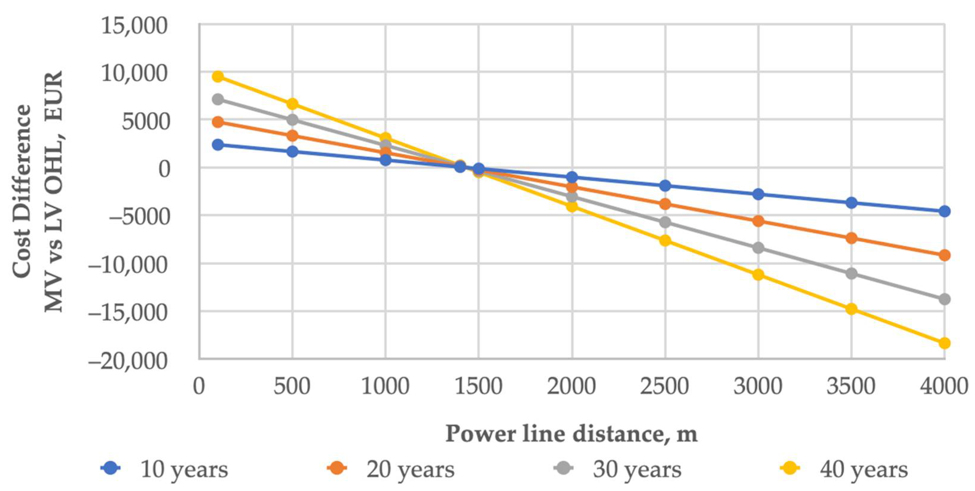
All calculations included fixed and variable costs of investment as well as operation and maintenance costs. In the presented feasibility studies, the costs of the line renovation options were reduced to one year. This reduction helps to calculate the total cost for different time periods (10, 20, 30, and 40 years) and at the same time, compare them for different line lengths (100–4000 m). The costs do not consider possible tariff reductions (due to poor service quality), inflation, or overall economic growths.

The analysis indicates, as expected, that in the case of low voltage line renovation, the lowest cost can be obtained with LV CS and the highest cost with LV OHL due to difference in life expectancy. The total costs of LV OHL and MV OHL become equal at line lengths of 1500 m (see Figure 1).

Therefore, in the case of power lines with lengths of more than 1500 m in areas where the long-term load prediction is increasing, it is more feasible to replace LV OHL with MV OHL. It is feasible to replace LV OHLs, which are shorter than 1500 m and located in areas without significant prospective load change, with LV CS. In areas where the long-term load prediction is decreasing and the lines are very long (i.e., over 4 km) but still a 40–year life expectancy is expected by the DSO, it is more viable to consider an off-grid solution instead. However, it should be noted that a detailed study must be carried out to validate the feasibility of such an investment.

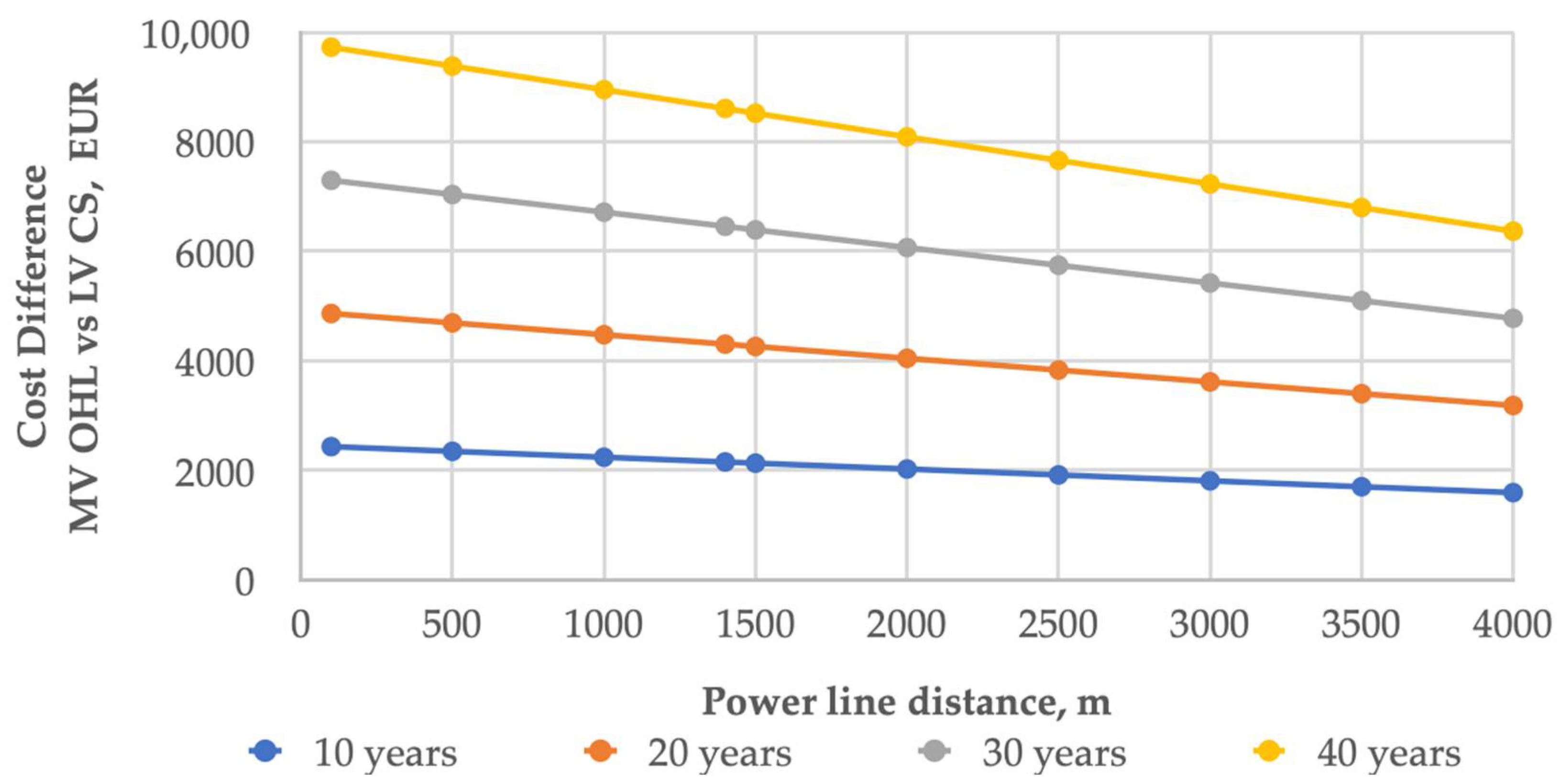
Based on the difference between the total investment costs of the MV OHL and the LV CS (Figure 2), it can be concluded that it would be feasible to replace LV CS with MV OHL only in the case of developing areas (long-term load prediction is increasing). For areas with a constant long-term load prediction, the total cost of LV CS is always lower than the total cost of MV OHL.

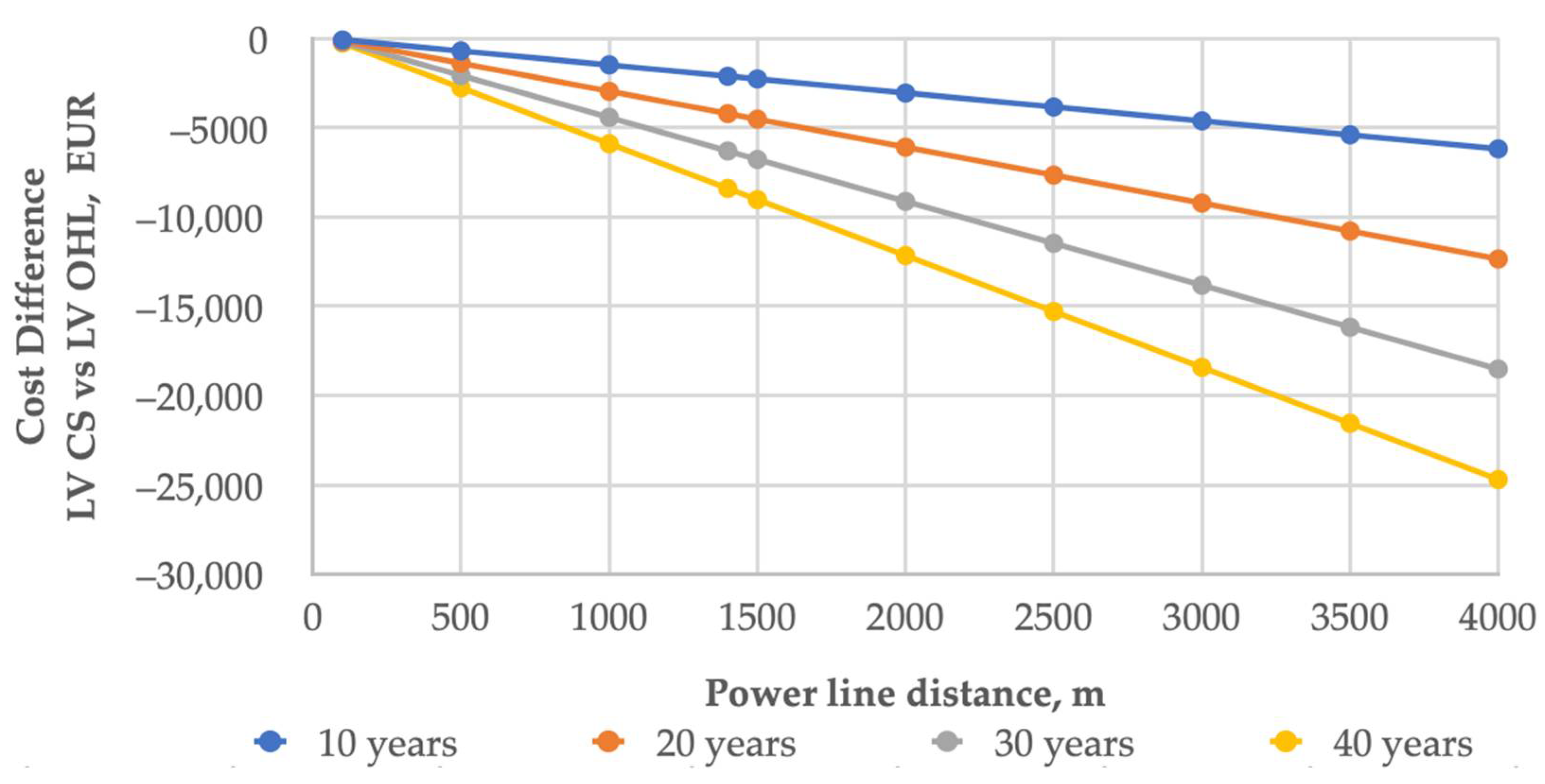
Based on the difference between the total costs of the LV CS and the total costs of the LV OHL (Figure 3), it is evident that it is always feasible to replace LV OHL with LV CS.

2.2. Voltage Stabilisers Compared to Power Line Renovation

Depending on the type of voltage problem and long-term load prediction, another feasible solution is to utilize the possibilities of voltage stabilisers or uninterruptible power supply (UPS) systems. If the long-term load prediction (over the next 40 years, which is the planned life expectancy of a power line) indicates constant or increasing load, then the LV OHL reconstruction/replacement with LV CS or MV OHL is always considered as an economically feasible solution.

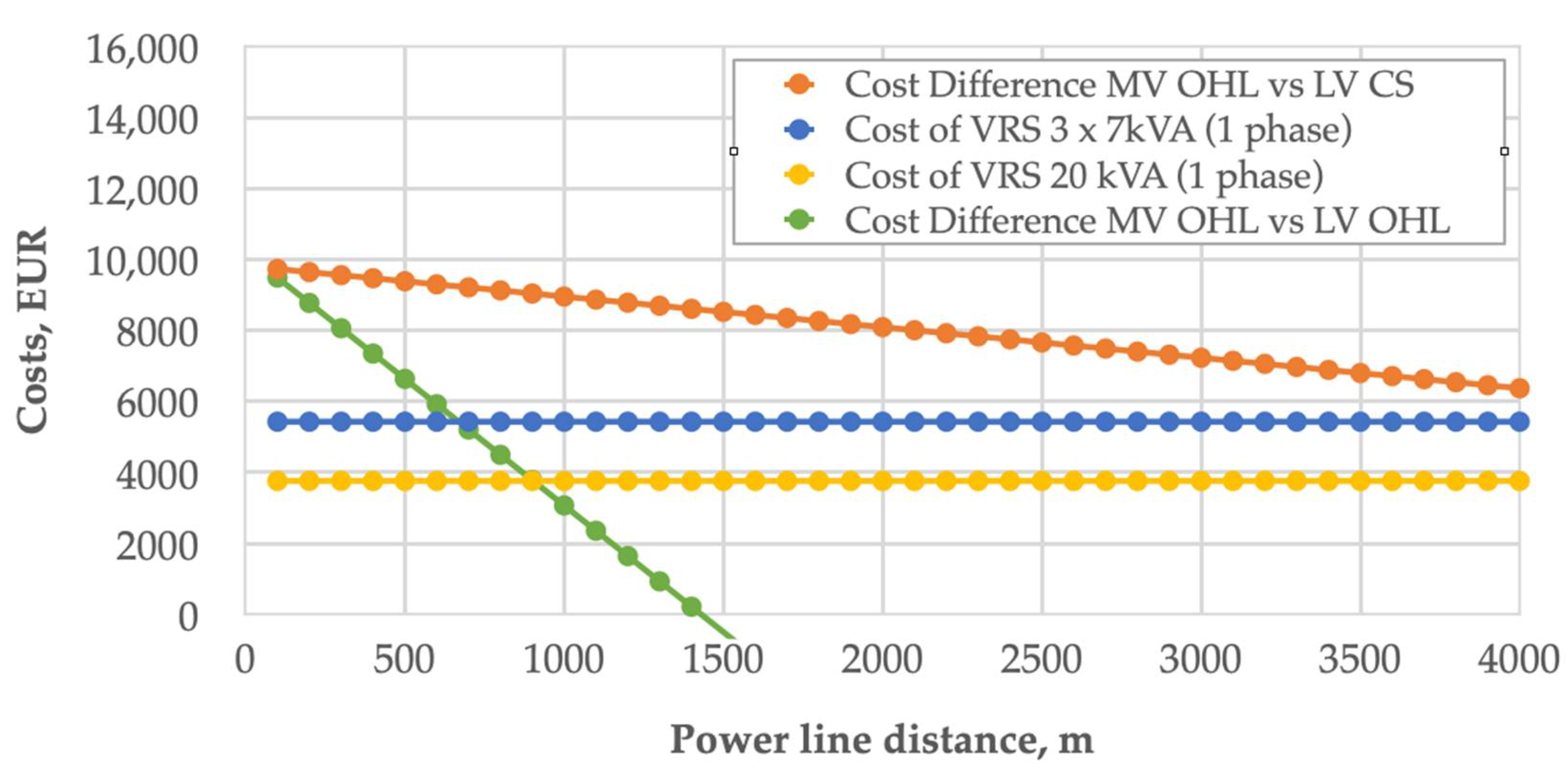
However, taking into consideration the total cost difference between MV OHL and LV CS over a 40–year period, it could be more feasible to use a voltage stabiliser to solve power quality related issues. According to the study in [31], the average consumer in areas with voltage problems is usually a one or three phase consumer with an average capacity between 20–30 kVA. Taking into consideration that voltage stabilisers in that capacity range are almost maintenance free and have an average cost of approximately 8000 euros [32], it is more feasible to use voltage stabilisers instead of MV OHL reconstruction if the distance remains below 2000 m and the consumers are connected through a three-phase point of common coupling (PCC) (Figure 4). However, depending on the voltage problem, the actual price of the voltage stabiliser may differ from the average price by up to 33%.

If the long-term load prediction shows a decrease in load, then with existing LV OHL or LV CS, the use of a voltage stabiliser is always recommended, since the total cost of the power line per unit of consumed electricity will increase due to declining electricity consumption.

2.3. Uninterruptible Power Supply and Supply Interruption Costs

A voltage stabiliser can only help to solve certain voltage problems (i.e., unbalance, voltage dips, or voltage swells), however, in the case of voltage interruptions, alternative devices would be a more feasible solution (e.g., UPS). According to [30], 65% of interruptions are shorter or equal to 3 min, and an average feeder can have approximately six to seven power outages annually.

In 2021, a survey on power quality and network service was conducted among service and industrial sector companies. The preliminary feedback from respondents indicated that the average loss due to power outages remains between 17,000 and 75,000 euros per day. Additionally, direct damage costs to equipment due to voltage problems are around 6000 euros per event. A similar conclusion can be made based on the survey [31] carried out by Leonardo Energy. According to preliminary feedback from the survey, customers who are sensitive to interruptions that are shorter than or equal to 3 min declared an average financial loss of approximately 39,400 euros per event. Depending on the customer and considering the average cost of a 20…30 kVA UPS system, a payback time between one and five years can be expected [33]. If the customer is highly sensitive to power quality related issues, the payback time could be even more attractive.

3. Classification and Description of Low Voltage Feeders for Simulations

The Estonian DSO’s internal standards on planning and operation foresee the assessment of voltage quality problems according to the European standard EN 50160 [34], specifically on slow voltage variations. Customers on low voltage feeders that are longer than 1500 m are defined to have voltage quality problems from a slow voltage variations point of view. Therefore, these customers are paying reduced network tariffs. Approximately 2000 feeders (ca 3%) of the total number of low voltage feeders are currently automatically considered to have problems with voltage quality [35]. However, this number may even be higher, as voltage quality issues may also be present in shorter distances from a substation.

Vill and Rosin describe the main topologies of the Estonian weak low voltage feeders in [35] based on the connection point (CP) placement and the average branching characteristics. Three typical topologies enable the classification of about 9% (6751 feeders) of the DSO’s low voltage feeders, which are highly likely to have voltage quality problems.

The topologies are identified by two parameters, which are calculated for every feeder in the sample. One parameter was a relation between an average connection point distance from the substation to the total length of the feeder. The second parameter was a relation between an average connection point distance from the closest branching point to the average CP distance from the substation. The three topology groups were named Group 1, Group 2, and Group 3.

These groups were then used to simulate the performance of the voltage stabilisers under different conditions with DIgSILENT PowerFactory software. The following sections provide a more detailed description of the groups and models.

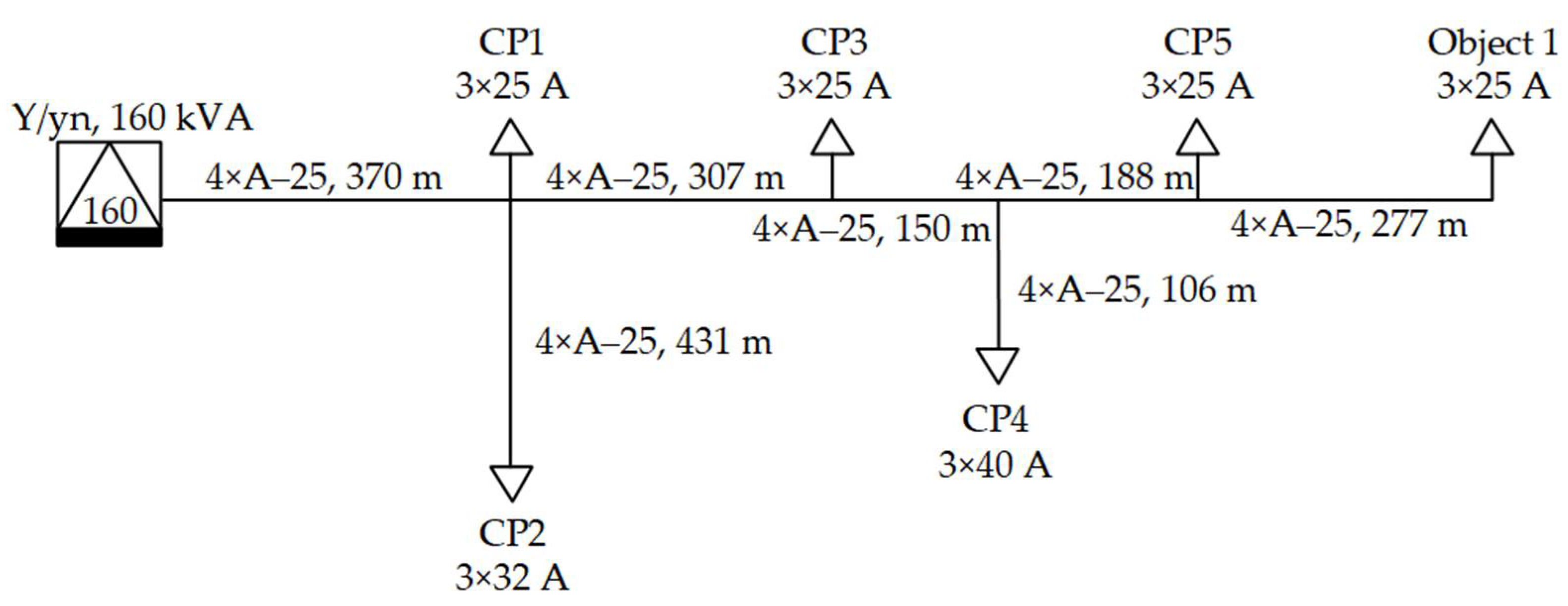
3.1. Group 1 Feeders

Group 1 classified feeders have on average 7–8 customer CPs. The load concentrates more on the first third of the feeder. This group has the most branches, and branching takes place on the first part of the feeder. The latter is the reason why this type of feeder is the longest. The average one-phase short-circuit impedance of connection points is the smallest among the three topology groups (1.29 Ω).

Grid 1 (Figure 5) represents an example feeder from Group 1, with the consumption centre located in the first third of the feeder. The substation consists of a 160 kVA 10/0.4 kV transformer with four connected low-voltage feeders. The feeder under investigation (F4) is an OHL with bare aluminium conductors (conductor type 4×A-25 and cross-section of 25 mm²) (Figure 5). The substation and power lines were built in the 1980s. The total yearly consumption of the F4 feeder is approximately 78,500 kWh, and the feeder has six CPs.

Measurements were conducted at the farthest connection point from the substation (Object 1 in Figure 5). Distance from the measurement point to the substation is 1.3 km. The connection point has a three-phase main fuse with 25 A rated current. The measured object’s yearly consumption is over 11,000 kWh.

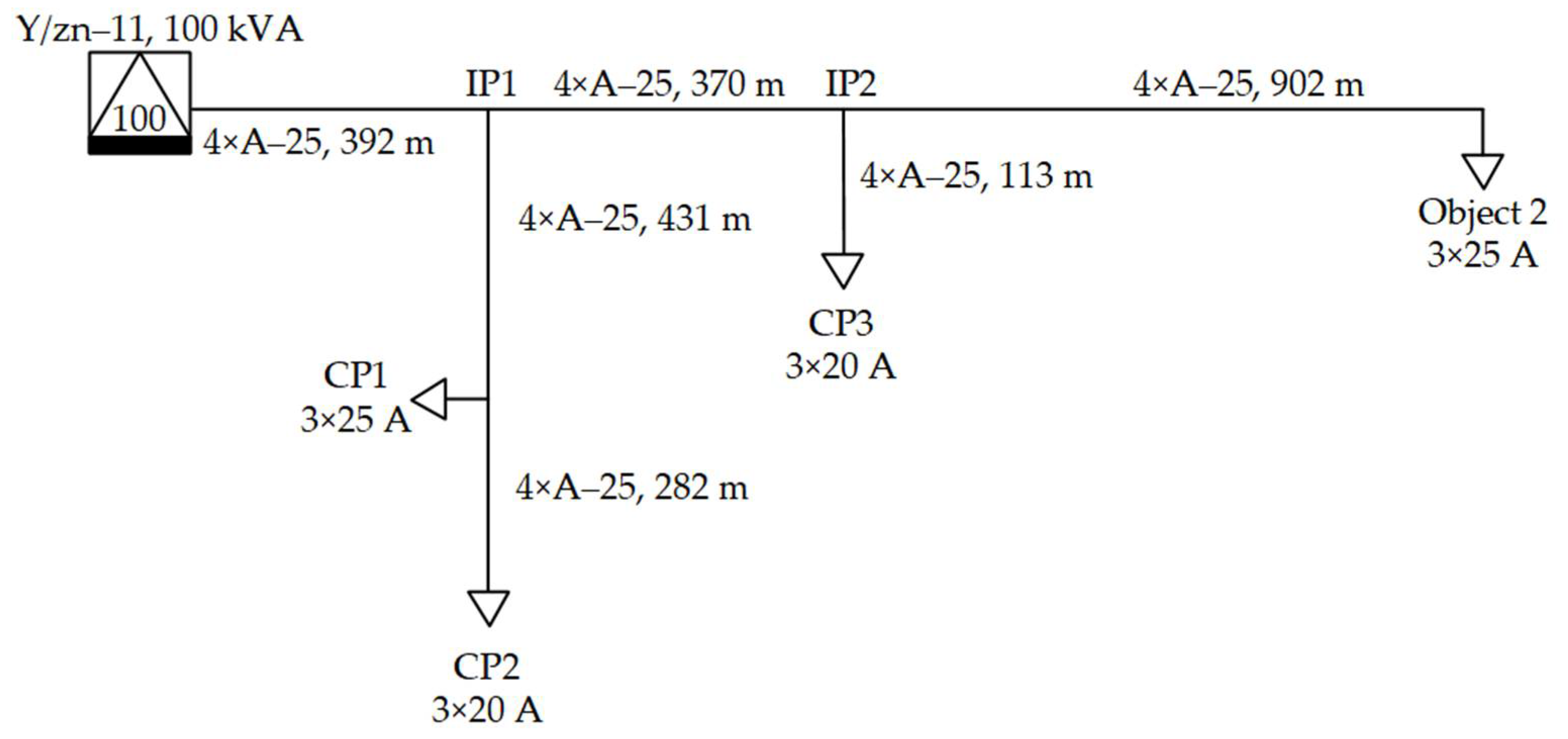
3.2. Group 2 Feeders

Group 2 classified feeders have on average four customer CPs and the load concentrates more on the second half of the feeder. A typical branch length is about 25% of the average distance from the substation to the CP. The average one-phase short-circuit impedance is 1.45 Ω and the majority (~40%) of the distribution feeders belong to this group. Grid 2 (Figure 6) represents an example feeder from Group 2.

The substation consists of a 100 kVA 10/0.4 kV transformer with three low-voltage feeders. The feeder under investigation (F2) is an OHL with bare aluminium conductors (conductor type 4×A-25 and cross-section of 25 mm²). The substation and power lines were built in the 1980s. The total yearly consumption of the F2 feeder is approximately 17,200 kWh, and the feeder has four CPs.

Measurements were conducted at the farthest connection point from the substation (Object 2 in Figure 6). Distance from the measurement point to the substation is 1.71 km. The connection point has a three-phase main fuse with a 25 A rated current, and the object’s yearly consumption is approximately 10,800 kWh.

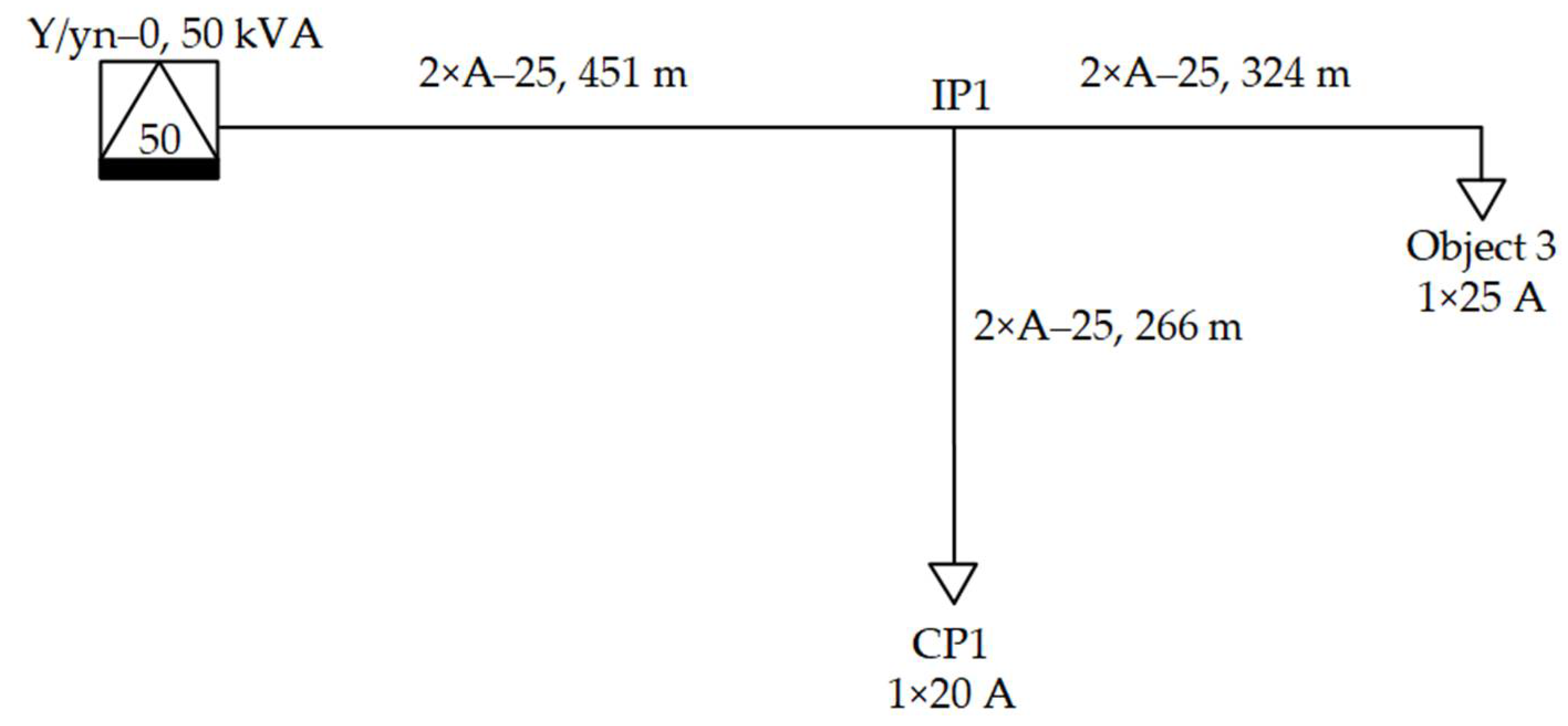
3.3. Group 3 Feeders

Group 3 classified feeders have on average only two customer CPs and the load concentrates more towards the last third of the feeder. The relative length of branches is the highest, constituting about 30% of the average distance from the substation to the CP. These feeders have the lowest total length with an average one-phase short-circuit impedance of 1.69 Ω. Grid 3 (Figure 7) represents an example feeder from Group 3.

The substation consists of a 50 kVA 10/0.4 kV transformer with three low-voltage feeders. The feeder under investigation (F3) is a single phase OHL with bare aluminium conductors (conductor type 2×A-25 and cross-section of 25 mm²) (Figure 7). The substation and power lines were built in 1977. The total yearly consumption of the F3 feeder is approximately 12,200 kWh, and the feeder has two CPs.

Measurements were conducted in the farthest connection point from the substation (Object 3 in Figure 7). Distance from the substation is 0.775 km. The connection point has a one-phase main fuse with a 25 A rated current, and the object’s yearly consumption is approximately 4700 kWh.

4. Voltage Quality Issues Discovered in the Sample Low Voltage Feeders

Power quality measurements were carried out in the sample objects’ customer CPs for initial data analysis and simulation. Measurement duration was one week, and the interval was one second. Additionally, the customers were interviewed about the perceivable voltage problems. Analysis of measurement results revealed that all three sample objects had common issues of high voltage fluctuation and intensive long-term flicker perceptibility. The latter exceeded the maximum value (determined in EN 50160) 2–4 times.

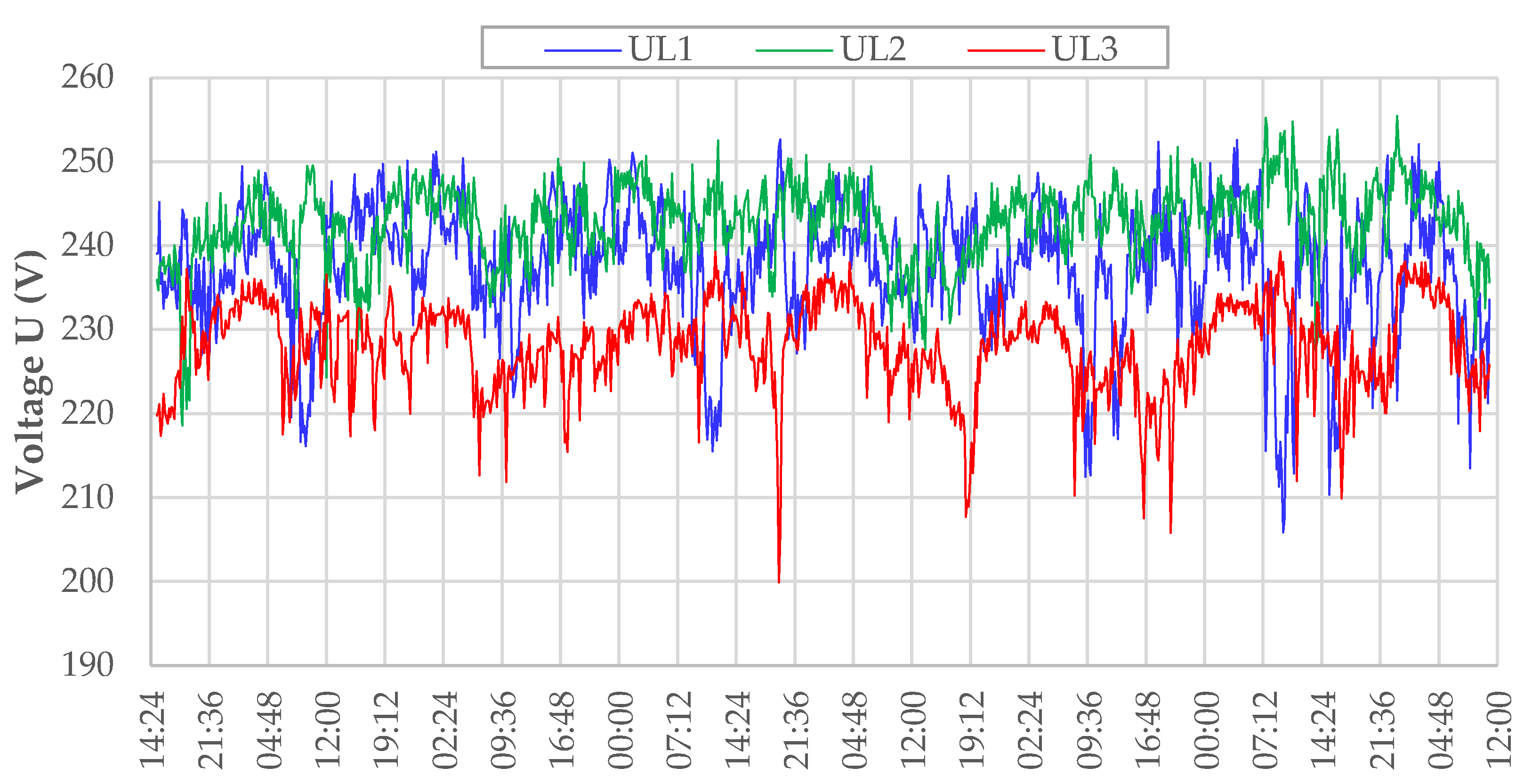
4.1. Object 1 Voltage Quality

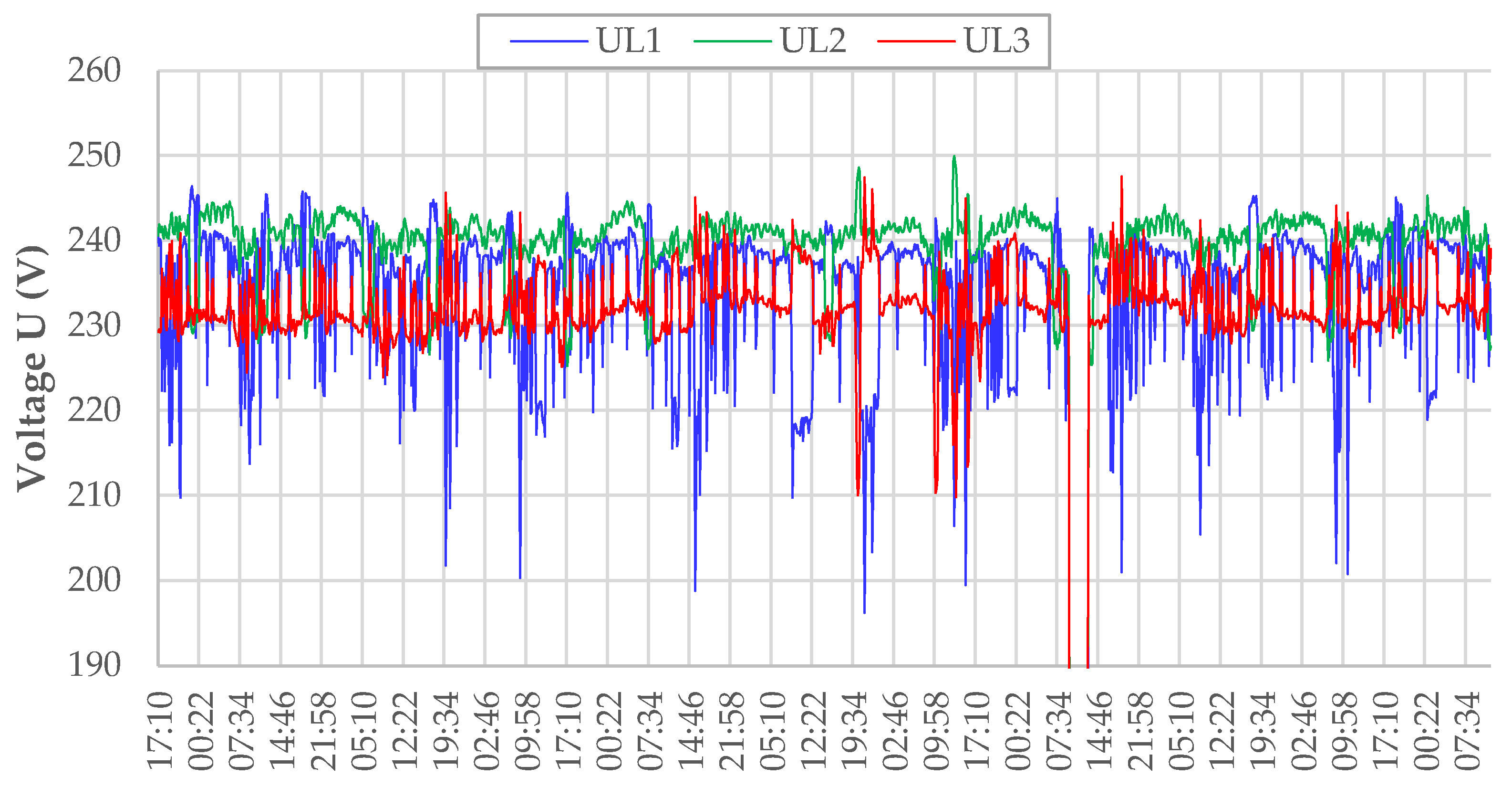
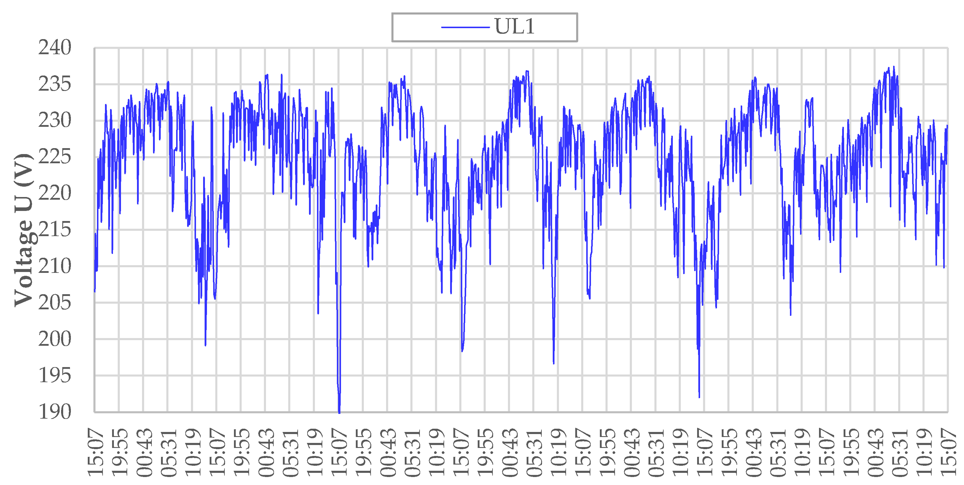
The measurements revealed that the average voltage level at Object 1 for one week was 235 V. At the same time, the voltage dispersion was very high: phase voltage remained between 200 V and 256 V. Although the voltage levels remained at 95% of the time within the standard requirements, such high variability can cause issues for the consumer and is at the same time visually detectable. Problems can be caused by higher single-phase loads or connecting multiple loads to a single phase, in this case, the voltage in phase can drop to 207 V, but at the same time, in another phase, it increased to 253 V. Figure 8 illustrates the measurement results for Object 1.

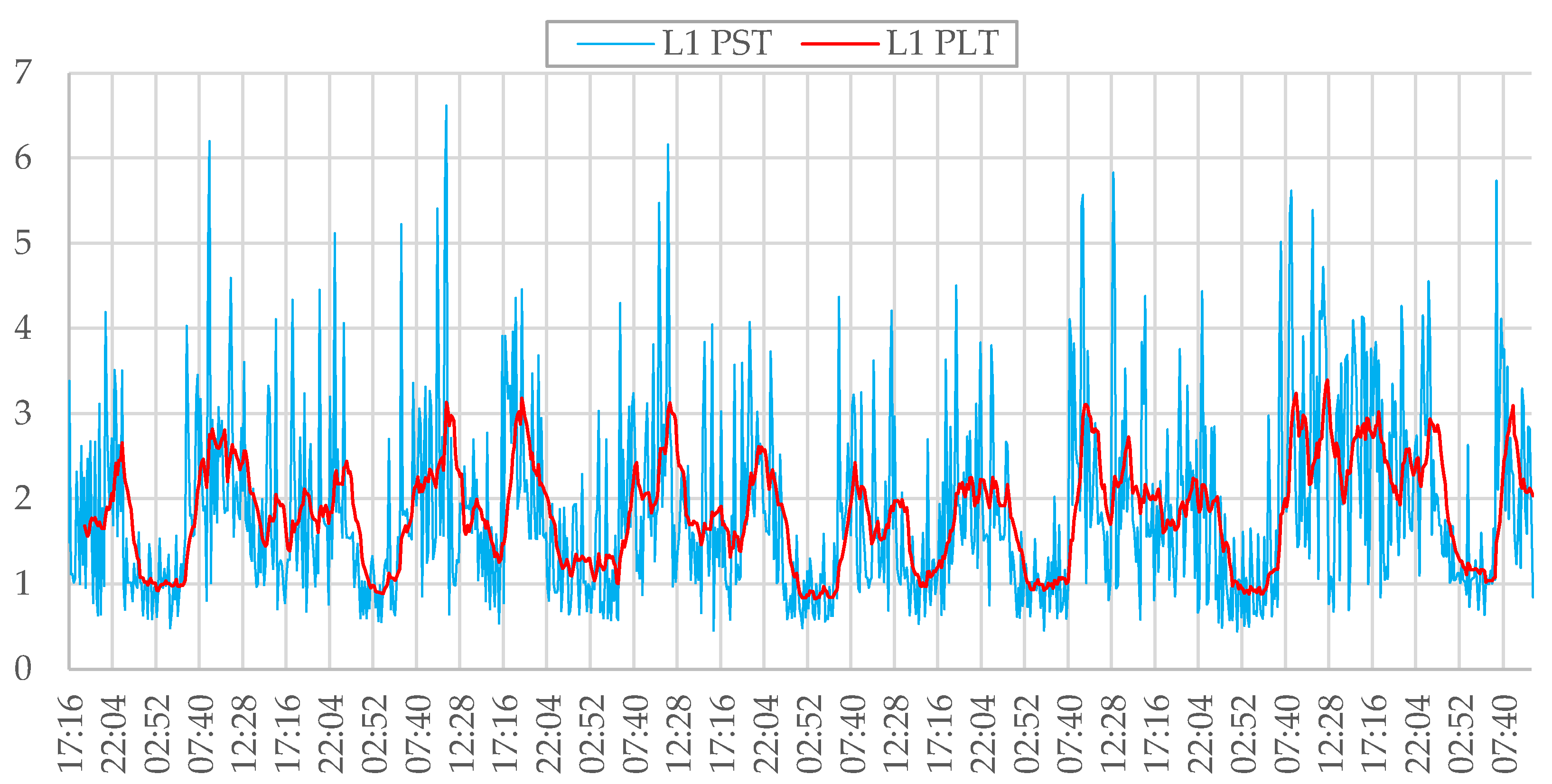
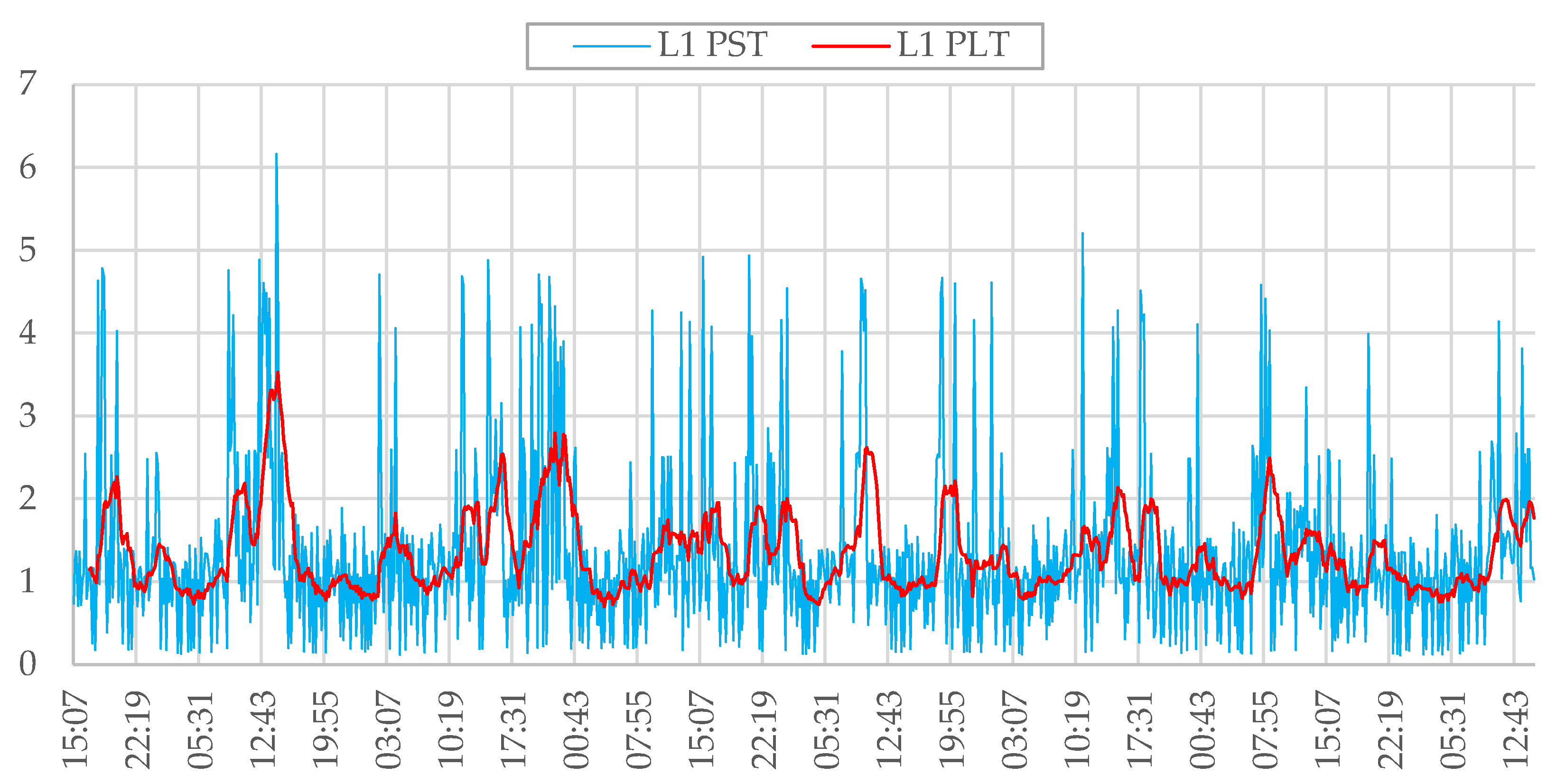
The large amplitude of variations can cause inconveniences to the customer and visually detectable changes in the luminous flux of luminaries, also known as flicker. The most disturbing flicker occurs in the frequency range of 8–9 Hz; frequencies above or below these values were less noticeable. In the current situation, the long-term flicker intensity remained between 0.8 and 3.5, and in the short-term up to 6.5, meaning that the recommended value of 1.0 according to EN 50160 is exceeded. Figure 9 illustrates the flicker measurements for Object 1, phase L1.

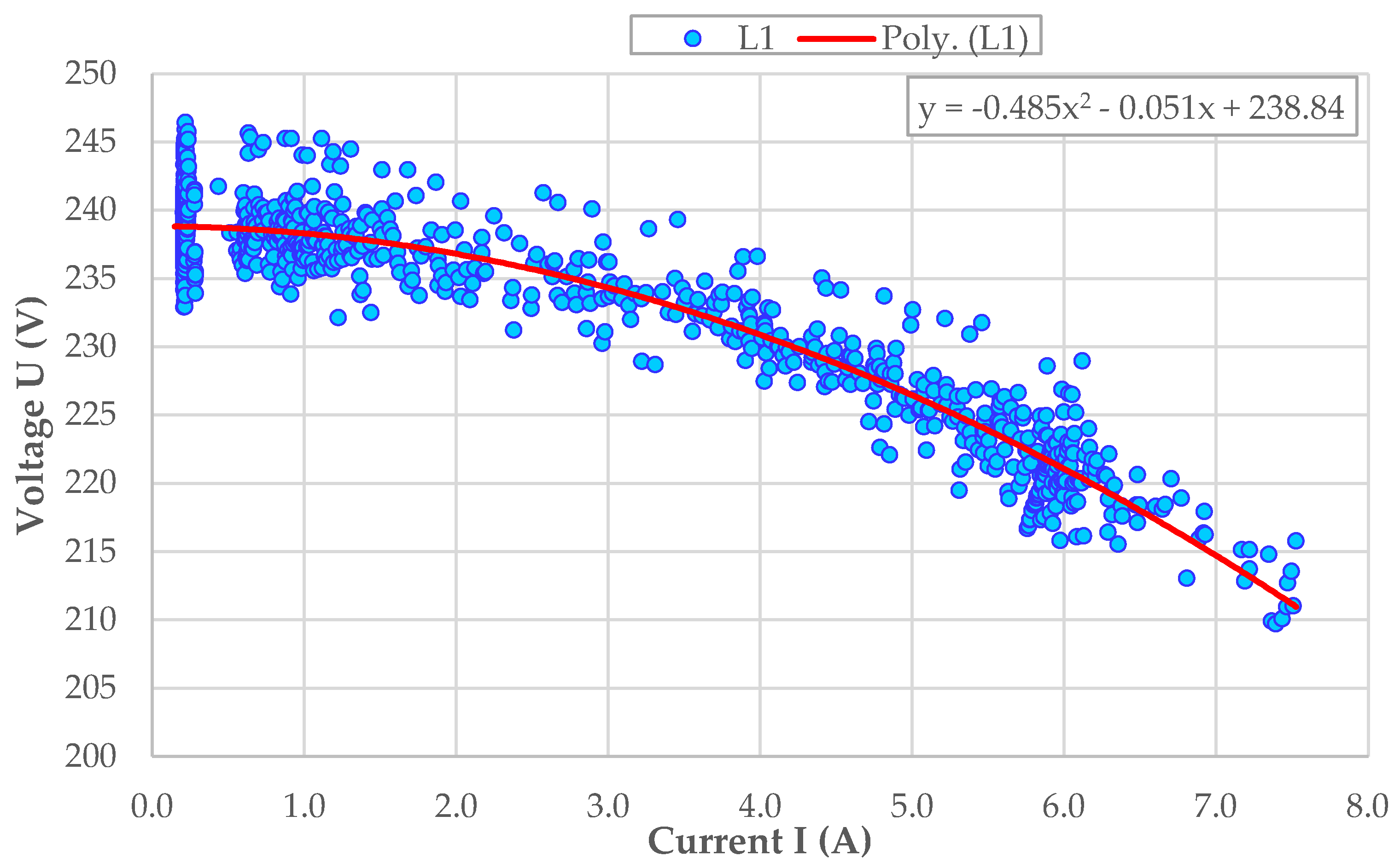
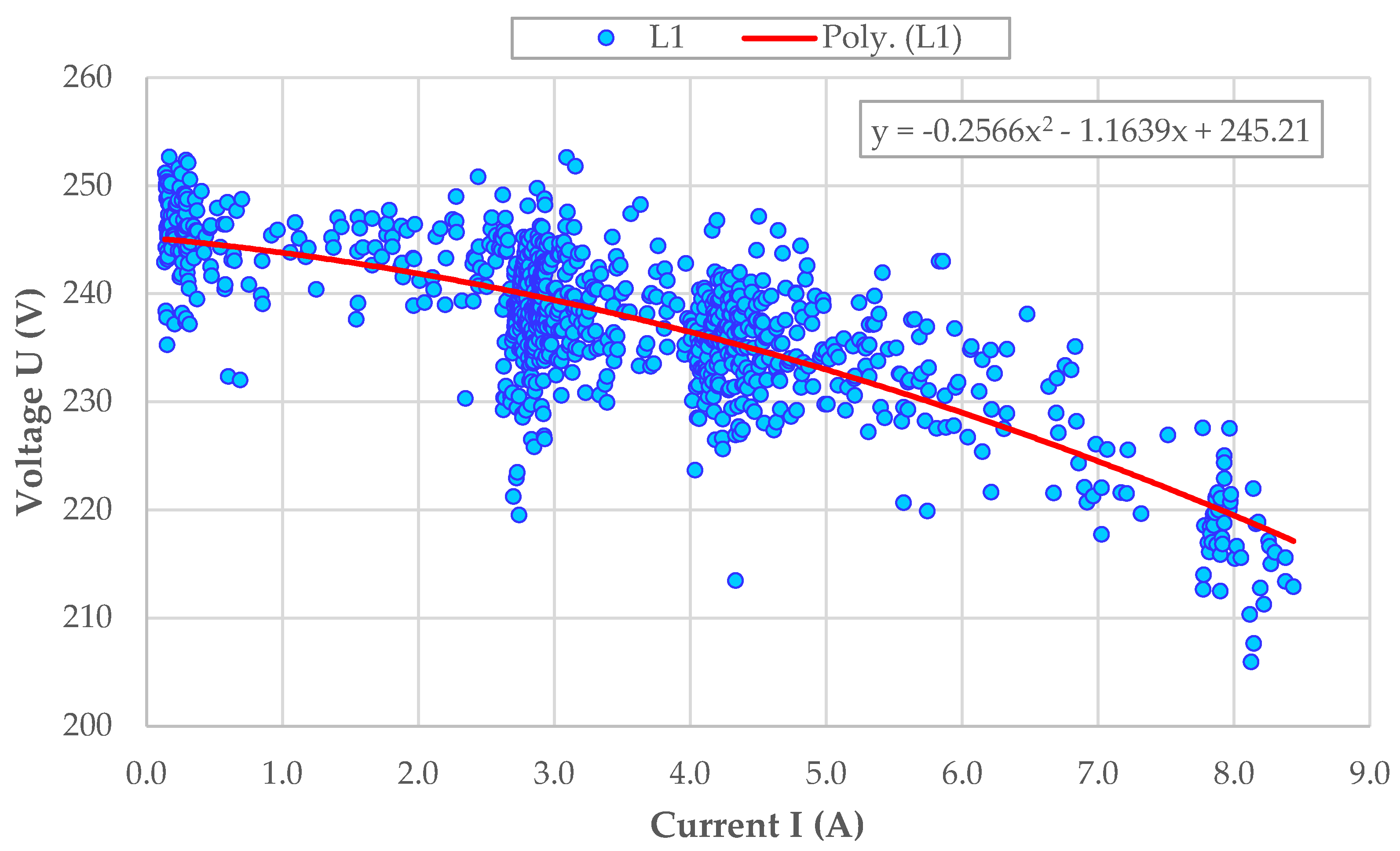
The most probable cause for the voltage quality issues are a high short-circuit impedance and voltage imbalance on the secondary side of the transformer. Figure 10 shows the voltage–current dependency curve of phase L1 derived directly from the measurement data at Object 1.

Based on the trend in Figure 8, this one-phase short-circuit impedance can be estimated for every phase using Equation (1):

$$Z_{LXN}\approx \frac{\Delta U_{LXN}}{\Delta I_{LXN}},$$

(1)

where Z_LXN is the phase X (representing either one, two or three) short-circuit impedance; ΔU_LXN is the voltage change for the corresponding phase between no-load and full load conditions; and ΔI_LXN is the current change for the corresponding phase between no-load and full load conditions. Results of the estimation are summarised in

Table 1. One-phase short-circuit impedance estimation for Object 1.

Phase L1, (Ω)	Phase L2, (Ω)	Phase L2, (Ω)
3.2	2.8	4.1

.

The calculated impedances were relatively high, meaning that a load current of 10 A will cause a 30 V voltage drop in the power line. According to the voltage limits set by the standard EN 50160, the maximum allowable load current at this customer CP was 10 A.

Additionally, numerous voltage sags and swells were detected in the measured CP. These sags and swells usually occur due to commutating some large electrical appliances, but also by short-circuit events in the high voltage grid. The detected voltage sags at Object 1 remained in the range of 170 V and with a duration over 100 ms. The most frequent sag durations were between 0.1–0.5 s and 3–60 s. The maximum detected voltage swell was 264 V with a duration over 100 ms. Most voltage swell durations remained between 3–60 s.

Additionally, the following voltage quality parameters were recorded and analysed for Object 1:

• voltage unbalance describes the relation of negative sequence voltage to positive sequence voltage, mainly affecting three phase motors by increasing their losses; and
• flicker is caused by systematic voltage waveform variations due to random voltage changes, causing perceivable light output variation in luminaries [36].

The results are summarised in

Table 2. Voltage unbalance and flicker measurement results for Object 1.

Parameter	EN 50160 Recommendations	Min	Max
Unbalance	2%	0.7%	3.3%
PLT	1	0.8	3.5

.

According to standard EN 50160, the maximum allowable values for voltage unbalance and flicker should not exceed 2% and 1, respectively. Furthermore, it is even recommended that the voltage unbalance remains below 1%. Flicker, on the other hand, is usually measured in two timeframes: short-term flicker perceptibility P_ST in a 10-min interval, and long-term flicker perceptibility P_LT in a 120-min interval. However, only the long-term flicker perceptibility is standardised. According to [8], in normal conditions, flicker perceptibility may not exceed the value P_LT = 1 in 95% of measured instances in a week. Long-term flicker perceptibility PLT at Object 1 was higher during daytime and lower at nights, while the short-term flicker perceptibility even reached as high as 6.7.

4.2. Object 2 Voltage Quality

The measurements in Object 2 also indicated a high voltage value dispersion. Voltage fluctuated between 196 V and 250 V with an average value of 236 V. The recorded values remained in the allowed range of 207–253 V in 95% of the measured time, as the standard requires, but such large deviations can cause similar issues as described for Object 1. Figure 11 illustrates the measurement results for Object 2.

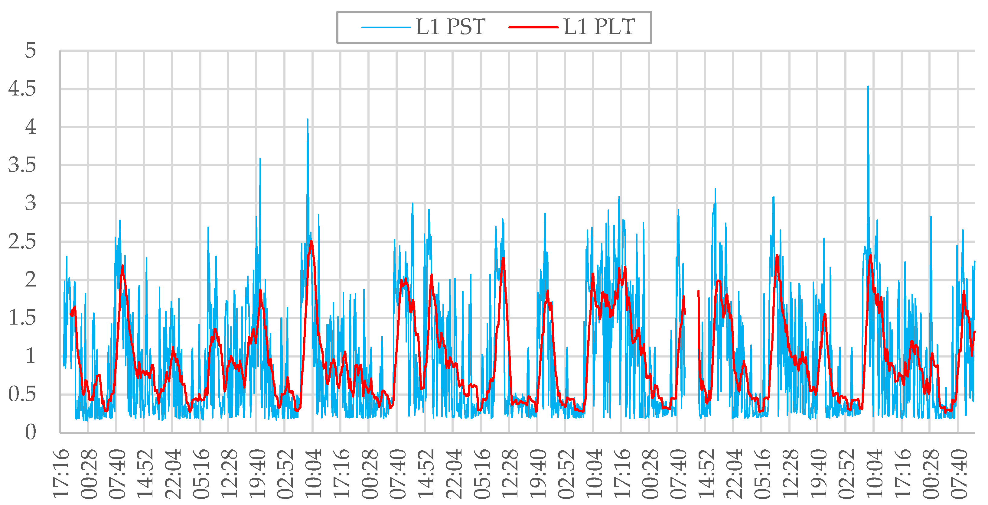
In the current case, the changes in the long-term luminous flux density for Object 2 remained between 0.3 and 2.5, however, the short-term flicker could exceed 4.5. The values recommended by standard EN 50160 are therefore well exceeded. Figure 12 illustrates the flicker measurements for Object 1 in phase L1.

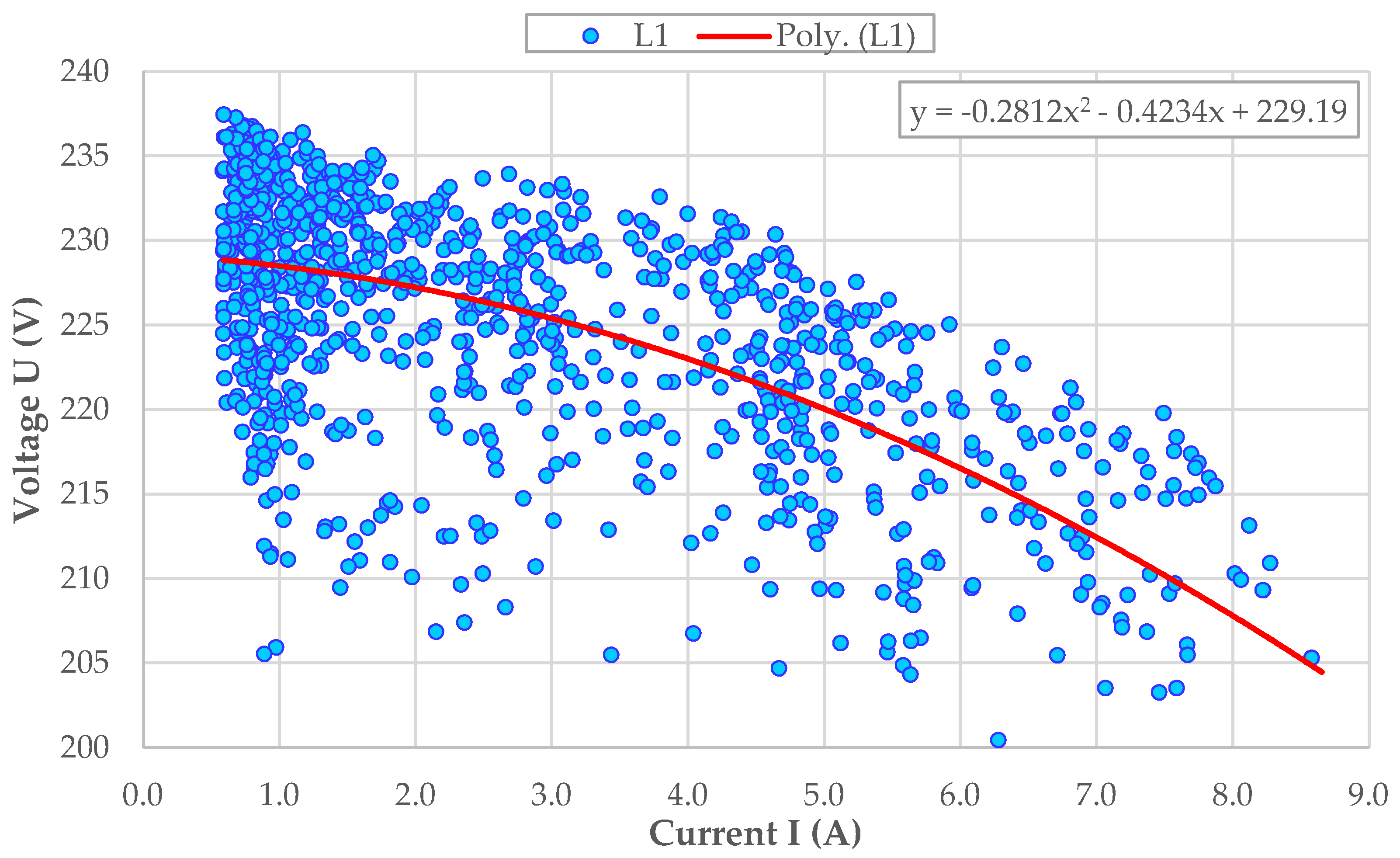
The most probable reason for the voltage quality issues is high short-circuit impedance or voltage unbalance on the secondary side of the transformer. Figure 13 presents a voltage–current dependency curve of phase L1 derived directly from the measurement data at Object 2.

Based on the curve in Figure 9, the one-phase short-circuit impedance can be estimated for every phase. The results are summarised in

Table 3. One-phase short-circuit impedance estimation for Object 2.

Phase L1, (Ω)	Phase L2, (Ω)	Phase L2, (Ω)
4.4	3.0	3.8

.

Calculated impedances were high, so at a load current of 10 A, a voltage drop in the power line was between 30 V to 44 V. Due to high short-circuit impedance at the connection point, maximum allowable phase current for this customer was also approximately 10 A at the CP. The recommended voltage unbalance and P_LT values also exceeded the EN 50160 standard values, and the results are summarised in

Table 4. Voltage unbalance and flicker measurement results for Object 2.

Parameter	EN 50160 Recommendations	Min	Max
Unbalance	2%	0.5%	3.9%
PLT	1	0.3	2.5

.

4.3. Object 3 Voltage Quality

Object 3 was situated on a one-phase feeder with a one-phase short-circuit impedance of approximately 2.1 Ω. The recorded voltage levels during the measurements remained between 183 V and 240 V, with an average value of 225 V. Similar to the previous objects, the values remained within the recommended limits of the EN 50160 standard, but such a large deviation can cause significant discomfort to the client. Figure 14 illustrates the measurement results for Object 3.

Due to high short-circuit impedance at the connection point (approximately two times higher than maximum recommended impedance value of 1 Ω), maximum allowable phase current for this customer was 16 A. Long-term flicker perceptibility PLT in phase 1 was between 0.8–3.4, being higher during the daytime and lower at nights. This exceeds the maximum value of 1.0 by EN 50160 considerably. Short-term flicker perceptibility was even higher and reached as high as 6.1, as illustrated in Figure 15.

Figure 16 shows a voltage–current dependency curve of phase L1 derived directly from the measurement data at Object 3, which was also used to estimate the above-mentioned one phase short-circuit impedance in the customer CP.

5. Description of Voltage Quality Improvement Devices for Simulations

According to the analysis of the measurement data of the three objects, the main power quality problems in the low-voltage grid were:

• short-term supply interruptions (up to 60 s);
• flicker;
• voltage dips; and
• voltage unbalance in the case of three-phase feeders.

Together with the DSO experts, the following voltage improvement devices were chosen for the simulations:

• dynamic voltage restorer (DVR), that are suitable for feeders with voltage dip and flicker problems;
• load balancing transformer (LBT) should be used in feeders with voltage unbalance issues, and;
• an UPS device is appropriate for feeders with various voltage problems including short-term supply interruptions.

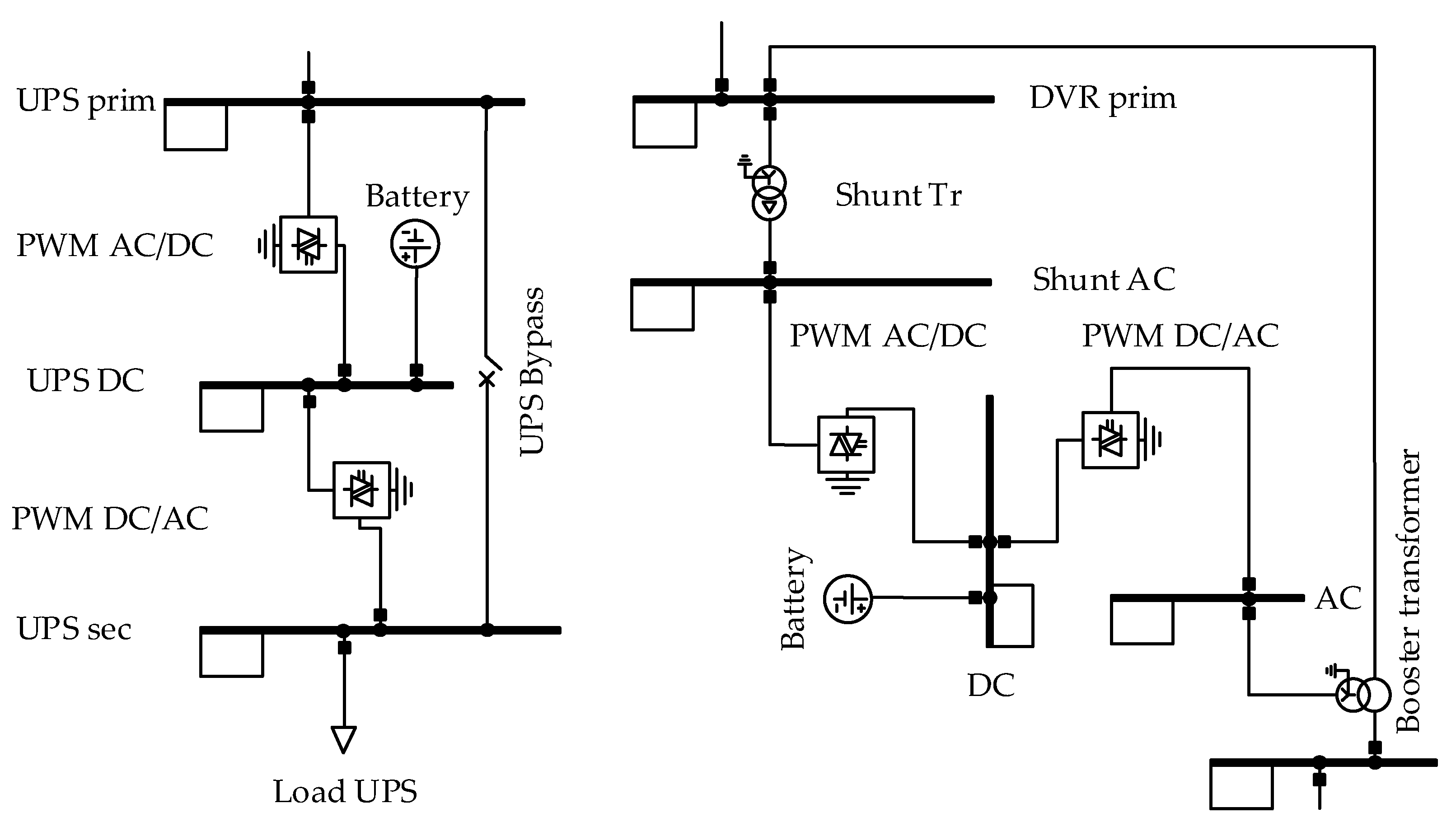
The models of the three different power quality improvement devices were created in PowerFactory software. UPS and DVR were built using predefined elements such as inverters, batteries, and booster transformer. The models created in PowerFactory for UPS and DVR devices are presented in Figure 17.

The UPS model consists of two pulse-width modulation (PWM) converters with an AC/DC/AC junction. The nominal DC voltage is UDC = 48 V. The capacity of the converters is taken same as the rated power of a transformer at the MV/LV substation. A universal type of battery is chosen, not considering the state of charge (SOC) characteristics and capacity. This simplification is acceptable, as at this stage, only the functionality of voltage regulation is needed.

The DVR model consists of a shunt transformer with a rated voltage on the secondary side of 60 V, two PWM converters with a DC rated voltage of 120 V, and a booster transformer. A battery was not used in simulations; however, it could be optional.

The third device, a LBT, was modelled based on an example, according to the manufacturer data in [37]. The load balancing transformer device EQUI8 redistributes loads and reduces asymmetry. EQUI8 balancing neutral current is equal to the voltage offset between real neutral and virtual neutral divided by EQUI8 resistance. The balancing current on each phase was 1/3 of the EQUI8 neutral current (flowing opposite). The amount of power as well as the direction of power were calculated in advance for each timestep in the simulation.

6. Simulation Results

To simulate the operation of the power grid, we used PowerFactory expansion stages tools. There is an option to change the grid structure (in our case, connect the voltage quality improvement device to as specific node) at a specific time. This means changing only the date, and the software carries out the simulations sequentially from the initial state to the improved state with devices. Such an approach reduces the calculation time and enables the comparison of results from different models and cases.

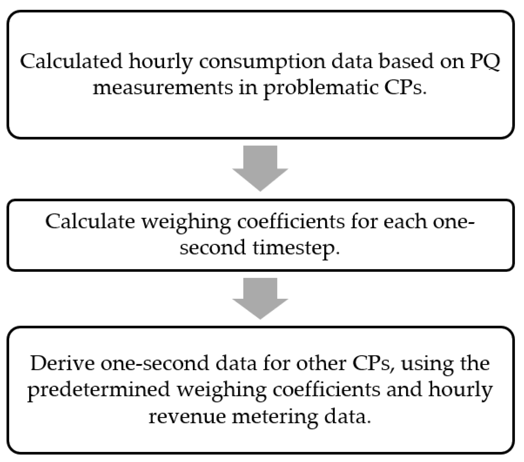
Since measurements were conducted only in the farthest CPs from the substation (Objects 1, 2, and 3), other CPs only have hourly data from revenue metering. For the simulations, the following method was used to create one-second data for simulations, as illustrated on Figure 18.

Such an approach amplifies any possible asymmetries and voltage problems and enables better estimation of the impacted devices of interest. Nevertheless, the authors acknowledge that it can also be considered as a drawback, since large voltage drops and increases reduce the convergence of power flow calculations. In practice, the simulated load asymmetry is rarely present. However, the advantage of such a methodology is beneficial when a feeder has a large amount of connection points, and the arrangement of simultaneous measurements is difficult.

The base case for the series of simulations was a model without any voltage quality improvement devices. The studied devices were placed in different connection points or branching points to determine their impact on the node voltages. For every studied voltage quality improvement device, several simulations were conducted to find an optimal placement of the device for every sample feeder.

Simulations were carried out using quasi-dynamic simulations (QDS). QDS allows for power flow calculations for different periods with the time step starting from one second. With the QDS feature, PowerFactory performs a power flow for a defined period and step, with a possibility of choosing parameters for the results.

In this study, we chose results to track phase voltages at each connection point. QDS was carried out based on the data measured on 8 November 2016 with a time step of 1 s for a period of 5 h (from 13:00 to 18:00). The nominal voltage 1 p.u. was taken as 230 V for phase-to-neutral voltage and 400 V for phase-to-phase voltage. The simulation was carried out with the Newton–Raphson solution engine, which is the most suitable for distribution grids with unbalanced loads. Voltage limits were disabled to avoid regulation through the external grid and clearly illustrate the deep drops.

6.1. Grid 1

From the results and analysis, it can be seen that placing the DVR device in CP1 is the best solution for Grid 1 (marked with a grey background in the table). Since the objects’ main issue is a low voltage level, the results present the minimum value of voltage during the simulation. Placing a UPS device at CP3 solves the voltage problem for Object 1 but does not solve the voltage problem at the connection point CP2. The LBT device in this case showed the worst performance because there was very strong load asymmetry with a similar profile in other connection points.

Unfortunately, the results showed that the voltage problem cannot be completely solved by these devices. One of the main reasons for not being able to solve the voltage problems are the artificially created difficult conditions (amplified asymmetry), which are rare in practice. The simulation results for Grid 1 are summarised in

Table 5. Comparison of solutions for Object 1.

Device Placement	Minimum Relative Voltage at Different Phases of Connection Points, p.u.
	CP2			CP4			Object1
	L1	L2	L3	L1	L2	L3	L1	L2	L3
Base Case	0.890	0.855	0.731	0.856	0.863	0.725	0.854	0.861	0.722
DVR at CP1	0.917	0.963	0.950	0.927	0.971	0.960	0.920	0.964	0.952
UPS at CP3	0.935	0.894	0.820	0.984	0.990	0.980	0.975	0.983	0.971
LBT at Object 1	0.864	0.908	0.896	0.977	0.914	0.899	0.871	0.909	0.895

.

6.2. Grid 2

The simulation results for Grid 2 are summarised in

Table 6. Comparison of solutions for Object 2.

Device Placement	Minimum Relative Voltage at Different Phases of Connection Points, p.u.
	CP2			Object 2
	L1	L2	L3	L1	L2	L3
Initial	0.910	0.909	0.895	0.854	0.853	0.827
DVR at IP2	0.973	0.974	0.974	0.957	0.962	0.956
UPS at Object 2	0.981	0.980	0.975	0.999	0.999	0.999
LBT at Object 2	0.972	0.974	0.964	0.970	0.970	0.960

. The results show that placing a UPS for Object 2 provides the best solution to solve the voltage problem. In contrast to the Grid 1 results, we can see that all devices provided satisfactory results even in the presence of artificially created strong load asymmetry.

6.3. Grid 3

Table 7. Comparison of solutions for Object 3.

Device Placement	Minimum Relative Voltage at Different Connection Points, p.u.
	CP1	Object 3
Initial	0.909	0.895
DVR at CP1	0.974	0.974
UPS at CP1	0.980	0.975
UPS at IP1	0.974	0.964

summarises the results of the Object 3 simulations. Although the distance of Object 3 from the substation exceeded that of CP1, then CP1 load had the highest impact on the voltage levels due to its high consumption. Therefore, it makes more sense to install a UPS device at CP1 than at Object 2. Similar results can be obtained if the UPS is installed at branching point IP1. The third device (LBT) was of no use, as the grid towards the end was a single-phase type.

7. Recommendations for Solving Voltage Problems

Based on the techno-economic analysis (in Section 2), this section summarises the possible solutions for solving voltage quality related issues for one or three phase consumers with an average capacity between 20–30 kVA (see Figure 4). The proposed solutions could be used for planning guidelines or additional features that new loads should incorporate when added to the urban distribution grids (i.e., chargers for e-mobility could incorporate devices that solve voltage problems similarly to DVR or LBT and energy storage systems as UPS).

Nevertheless, when solving voltage problems in low voltage grids, several aspects should be considered:

• feeder reconstruction plans;
• condition and lifetime expectation of existing substation and its components;
• type, length, and life expectance of power lines;
• long-term load forecasts and types of loads (three-phase, unbalanced, electronic, etc.); and
• existing and future PQ problems.

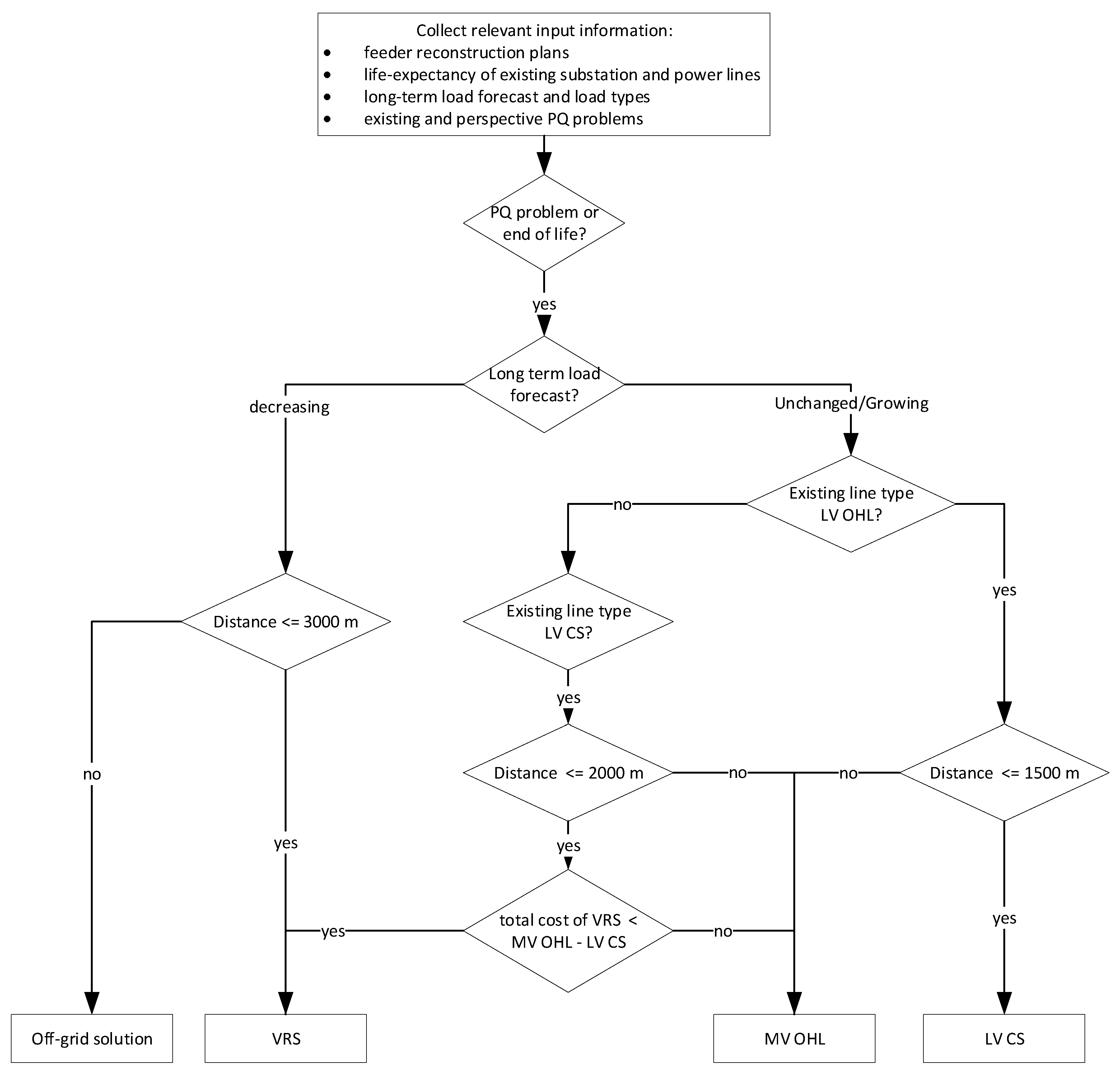
The following recommendation was formulated based on the analysis carried out in the previous sections, and considered the feasibility study of line types, voltage regulation systems (stabilisers, UPS, etc.), types of voltage problems, and long-term prediction of power consumption. If the LV OHL is nearing the end of its useful life or has a voltage problem, the following recommendations are actual:

• for network segments with feeder lengths up to 3 km and where the long-term load forecast is decreasing, installing a DVR should be considered;
• for network segments with feeder lengths of over 3 km and where the long-term load forecast is decreasing, an off-grid solution should be considered;
• for network segments with feeder lengths up to 1.5 km and where the long-term load forecast is relatively constant, the replacement of existing lines with LV CS should be considered; and
• for network segments with feeder lengths of over 1.5 km and where the long-term load forecast is increasing, the replacement of existing lines with MV OHL should be considered.

If the LV CS is nearing the end of its useful life or has a voltage problem, the following recommendations are actual:

• for network segments with feeder lengths not exceeding 2 km and where the long-term load forecast remains unchanged, a voltage regulating system (VRS) should be considered in the case the total cost over the full lifetime does not exceed the difference between the total costs of the MV OHL and the LV CS;
• for network segments with feeder lengths over 3 km and where the long-term load forecast is decreasing, an off-grid solution should be considered; and
• for network segments with feeder lengths over 2 km and where the long-term forecast remains relatively constant, the replacement of the existing lines with MV OHL should be considered.

In terms of fast performance (a few milliseconds) and lifetime, stepwise adjustable stabilisers with static or semiconductor switches are recommended. In the case of longer dips, electromagnetic voltage boosters can also be considered. The use of voltage stabilisers is recommended in situations where voltage fluctuations are within ±20% of the rated voltage (Un). In the case of strong voltage fluctuations, the prices of the voltage stabiliser increase significantly. For example, a shift from ±20% Un to ±40% Un means an increase in price by two-fold. In the case of supply interruption or strong voltage fluctuation, a UPS is the most feasible solution. The respective recommendations and the suitability of different voltage regulation systems as a solution for different voltage quality issues are summarised in

Table 8. Summary of the recommendations to solve voltage problems.

Long-Term Load Forecast	Existing Line Type	Recommended Solution Based on Distance, m
		0…1500	1501…2000	2001…3000	>3000
Decreasing	LV OHL	VRS	VRS	VRS	Off-grid
	LV CS	VRS	VRS	VRS	Off-grid
Standing/unchanged	LV OHL	LV CS	MV OHL	MV OHL	MV OHL
	LV CS	Other	Other	MV OHL	MV OHL
Growing	LV OHL	LV CS	MV OHL	MV OHL	MV OHL
	LV CS	Other	Other	MV OHL	MV OHL

LV OHL—low voltage bare wire overhead line. VRS—voltage stabiliser/voltage regulation system. LV CS—uninsulated messenger cable system. MV OHL—medium voltage bare wire overhead line. Off-grid—local power generation solution with energy storage. Other—if total costs of VRS < (MV OHL–LV CS), then VRS, else MV OHL.

and

Table 9. Recommended voltage regulation systems for different voltage quality related issues.

Description	Criteria	Solution	Location
Voltage unbalance in phases (asymmetry)		Asymmetry balancing device/transformer	Near object
Voltage dip/swell	Within ±20–40%Un,	Electronic or electromagnetic voltage restorer/stabiliser/ booster or dynamic voltage restorer	Near object or weighted centre of load
Supply interruption, strong voltage fluctuations, transient overvoltage, frequency problems, etc.	>±40%Un	On-line UPS, dynamic voltage restorers with storage	Near object or weighted centre of load

. A flowchart to select the recommended solution is provided in Figure A1 of Appendix A.

8. Conclusions and Future Work

Based on the simulations, no single universal solution is possible that enables mitigating all the voltage problems at once. Suitable solutions depend on voltage unbalance, load characteristics, and length of the power line. However, the UPS has several advantages over other devices. Additionally, the UPS suits best where frequent power interruptions take place and numerous customers are connected. LBT is the best in cases where voltage is well balanced, and the number of interruptions is low. DVR suits best in power lines with many branches and a small number of interruptions. Furthermore, it is essential that the voltage sags do not fall below 40% of U_n.

The main aspects to consider in planning investments in power quality improvement devices are the location of the load centre and the long-term load forecast. In situations where the load centre is in the first third of the feeder, but the voltage problem manifests in the farthest point, a DVR should be placed in the load centre. The UPS solution is the most preferable solution for voltage problems in the case the load centre is located more on the second half of the feeder, and voltage related issues include frequent interruptions and large voltage fluctuations. In the case of voltage imbalance issues, the first solution should be to equalise the load between phases in the customer’s facility. Should the problem persist, a LBT-type device should be installed near the problematic site.

The presented paper focuses on the possible voltage problems in low voltage distribution grids and their respective solutions. This is an essential foundation for the future work that will focus on studying the possibility of utilising unused urban infrastructure (e.g., street lighting feeders) to provide novel and flexible public services. The analysed problems will be an actual problem in the urban distribution grids as the changing climate and the European Union legislation will drive the increased need for e-mobility related services. Since the distribution networks near metropolises already have a capacity shortage, innovative solutions are required to accommodate additional loads without significant investment into new electricity networks. One possibility is the use of underutilised urban infrastructure. The study summarised in this paper is an essential input to foresee the possible problems that might arise and their respective solutions. Considering the rapid development of power electronic devices, some, if not all, of the analysed VRS possibilities could be integrated into energy storage systems and e-mobility chargers to solve possible voltage quality issues.