Figure 1.
LP-ESC: Conventional ESC with log power feedback.
Figure 1.
LP-ESC: Conventional ESC with log power feedback.
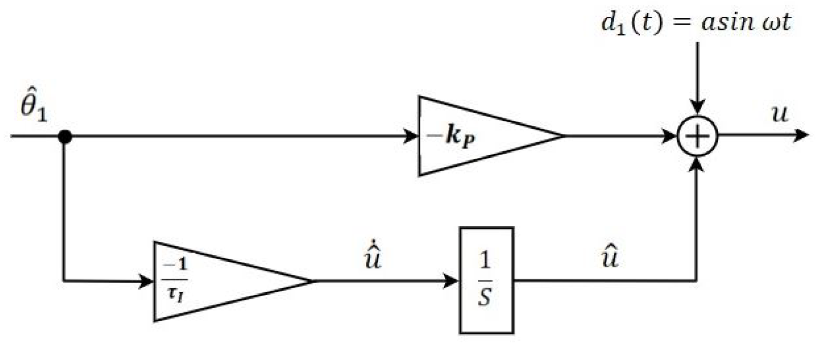
Figure 2.
PI controller used for LP-PIESC.
Figure 2.
PI controller used for LP-PIESC.
Figure 3.
LP-ESC/LP-PIESC implementation.
Figure 3.
LP-ESC/LP-PIESC implementation.
Figure 4.
Rotor speed dynamics for step changes in u ( m/s).
Figure 4.
Rotor speed dynamics for step changes in u ( m/s).
Figure 5.
Bode Plot of input dynamics, LPF, HPF, and the dither frequency.
Figure 5.
Bode Plot of input dynamics, LPF, HPF, and the dither frequency.
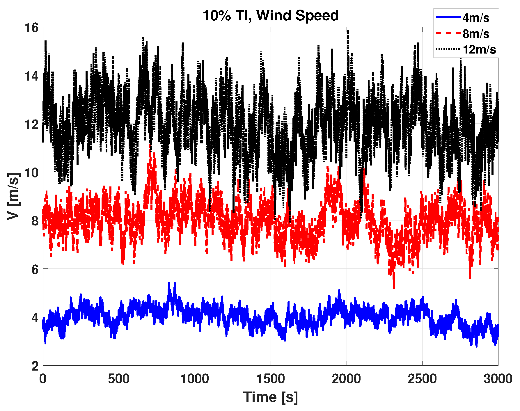
Figure 6.
Wind speed time series at hub height: mean wind speeds 4 m/s, 8 m/s, 12 m/s and 10% turbulence intensity.
Figure 6.
Wind speed time series at hub height: mean wind speeds 4 m/s, 8 m/s, 12 m/s and 10% turbulence intensity.
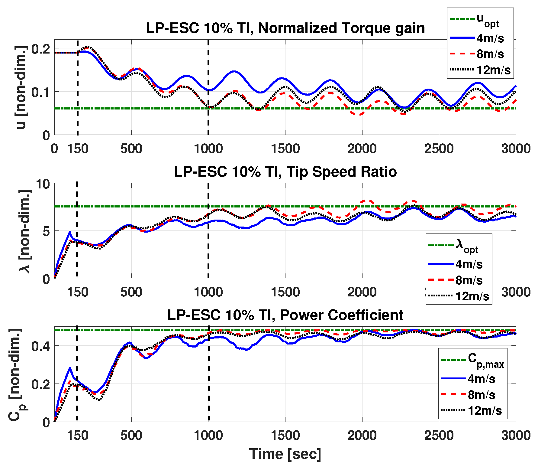
Figure 7.
Performance of LP-ESC with the parameters shown in
Table 2 and hub-height wind from
Figure 6. Normalized torque gain
u (
top), tip speed ratio
(
middle), estimated power coefficient
(
bottom). The dashed horizontal lines indicate optimal parameters
,
and
. Vertical dashed lines in
u show the point LP-ESC is turned on (150 s) and the point where it reaches practical convergence.
Figure 8.
Performance of LP-PIESC with the parameters shown in
Table 3 and hub-height wind from
Figure 6. Normalized torque gain
u (
top), tip speed ratio
(
middle), estimated power coefficient
(
bottom). The dashed horizontal lines indicate optimal parameters
,
and
. The LP-PIESC is turned on at 150 s.
Figure 9.
Performance of LP-PIESC with the parameters shown in
Table 3 and wind input with 15% TI. Normalized torque gain
u (
top), tip speed ratio
(
middle), and estimated power coefficient
(
bottom). The dashed horizontal lines indicate optimal parameters
,
and
. The LP-PIESC is turned on at 150 s.
Figure 10.
Energy capture comparison: Baseline vs. LP-ESC. Average energy output with baseline optimal torque gain and LP-ESC (top), percentage change in energy capture (bottom).
Figure 10.
Energy capture comparison: Baseline vs. LP-ESC. Average energy output with baseline optimal torque gain and LP-ESC (top), percentage change in energy capture (bottom).
Figure 11.
Energy capture comparison: Baseline vs. LP-PIESC. Average energy output with baseline optimal torque gain and LP-PIESC (top), percentage change in energy capture (bottom).
Figure 11.
Energy capture comparison: Baseline vs. LP-PIESC. Average energy output with baseline optimal torque gain and LP-PIESC (top), percentage change in energy capture (bottom).
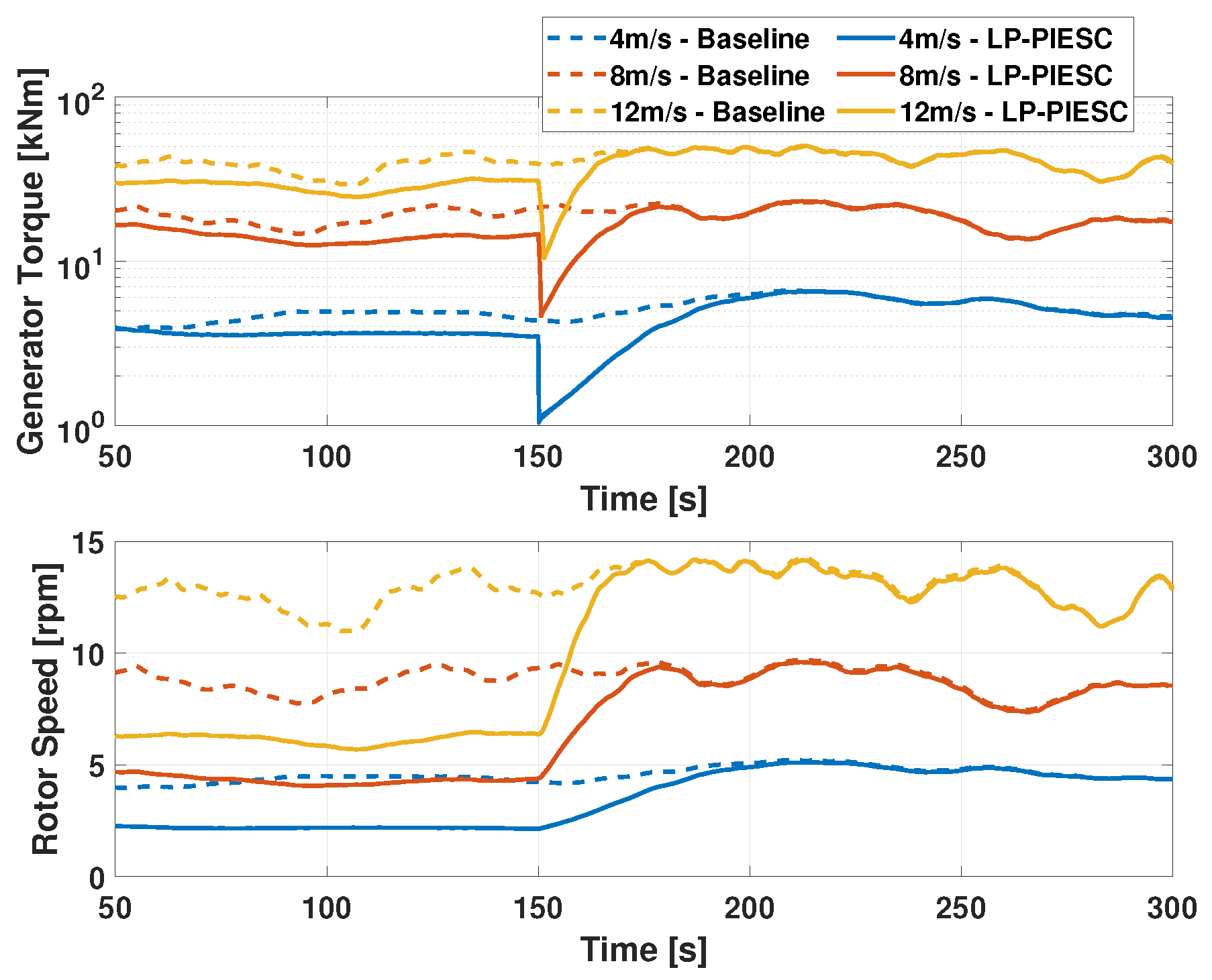
Figure 12.
Effect of sudden change in torque gain with LP-PIESC on generator torque (
top) and rotor speed (
bottom) compared with the baseline (for hub height wind from
Figure 6).
Figure 12.
Effect of sudden change in torque gain with LP-PIESC on generator torque (
top) and rotor speed (
bottom) compared with the baseline (for hub height wind from
Figure 6).
Figure 13.
Drivetrain torsion comparison: Baseline vs. LP-PIESC. Aggregate DEL values with baseline controller and LP-PIESC (top), percentage change in DEL (bottom) for time series from 150 s to 3000 s.
Figure 13.
Drivetrain torsion comparison: Baseline vs. LP-PIESC. Aggregate DEL values with baseline controller and LP-PIESC (top), percentage change in DEL (bottom) for time series from 150 s to 3000 s.
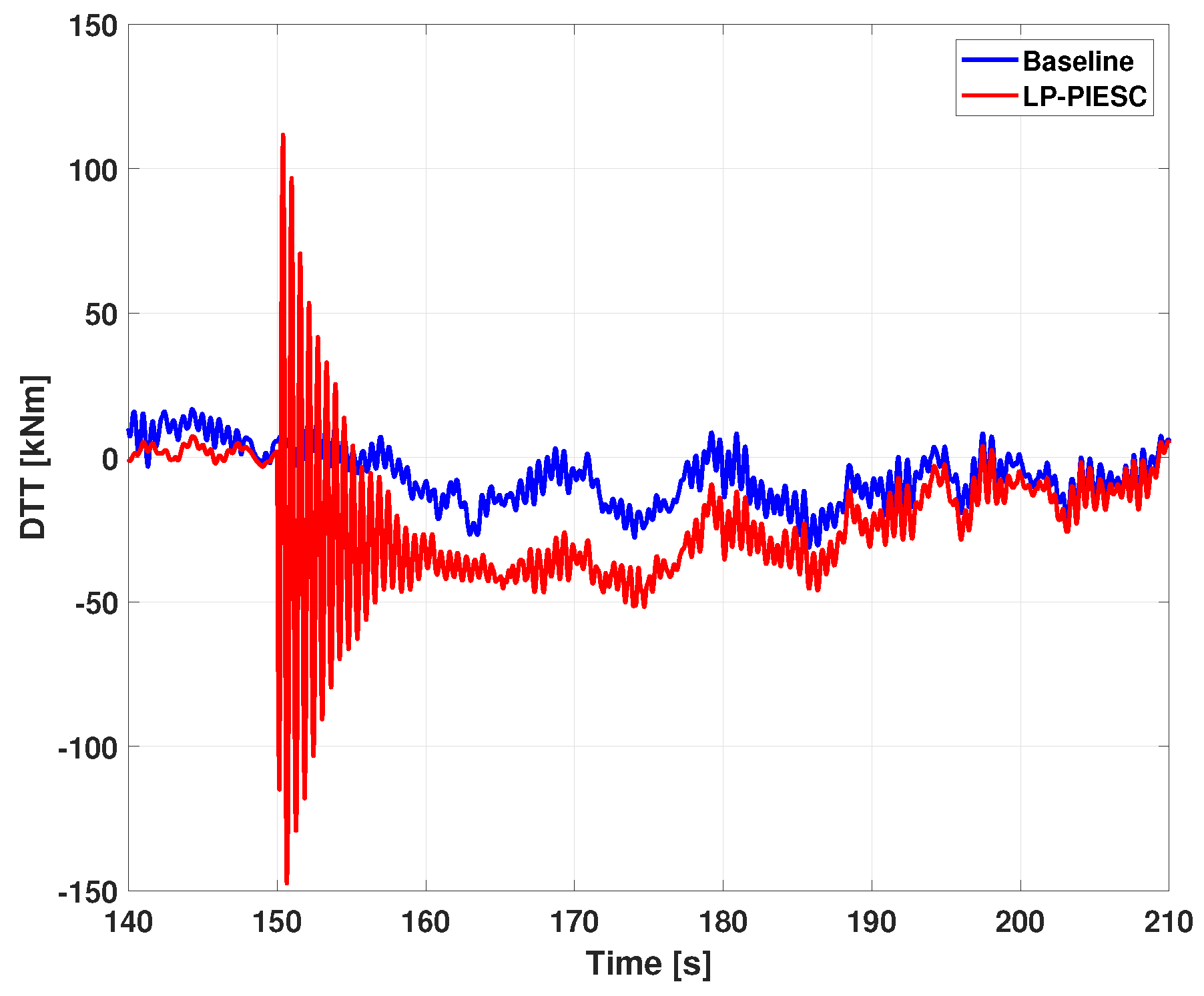
Figure 14.
Drivetrain Torsion (DTT) time series of baseline (blue) and LP-PIESC (red) for the 4 m/s wind profile in
Figure 6. Sudden change in generator torque at LP-PIESC start, i.e., 150 s leads to an increase in the amplitude of the drivetrain torsional moment. Once the transients die out, it follows the baseline.
Figure 15.
Drivetrain torsion comparison: Baseline vs. LP-PIESC. Aggregate DEL values with baseline controller and LP-PIESC (top), and percentage change in DEL (bottom) for time series from 300 s to 3000 s.
Figure 15.
Drivetrain torsion comparison: Baseline vs. LP-PIESC. Aggregate DEL values with baseline controller and LP-PIESC (top), and percentage change in DEL (bottom) for time series from 300 s to 3000 s.
Figure 16.
Tower- base fore-aft bending moment comparison: Baseline vs. LP-PIESC. Aggregate DEL values with baseline controller and LP-PIESC (top), percentage change in DEL for time series from 150 s to 3000 s.
Figure 16.
Tower- base fore-aft bending moment comparison: Baseline vs. LP-PIESC. Aggregate DEL values with baseline controller and LP-PIESC (top), percentage change in DEL for time series from 150 s to 3000 s.
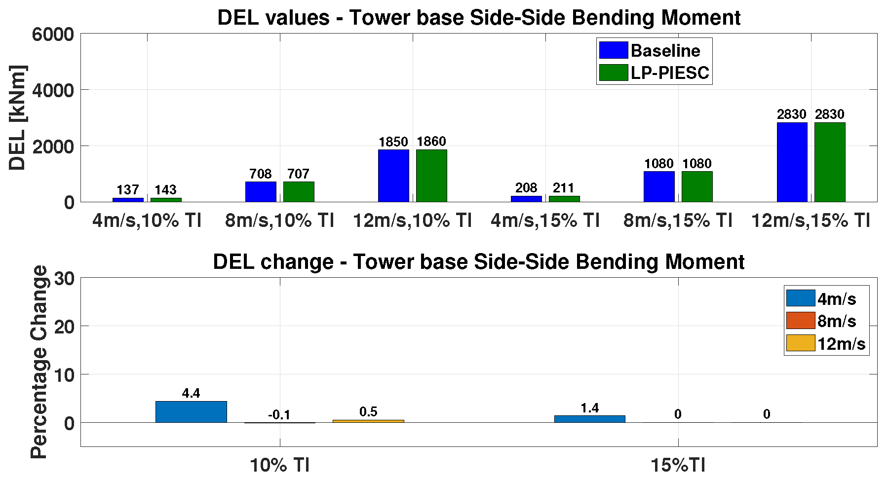
Figure 17.
Tower-base side-side bending moment comparison: Baseline vs. LP-PIESC. Aggregate DEL values with baseline controller and LP-PIESC (top), percentage change in DEL (bottom) for time series from 150 s to 3000 s.
Figure 17.
Tower-base side-side bending moment comparison: Baseline vs. LP-PIESC. Aggregate DEL values with baseline controller and LP-PIESC (top), percentage change in DEL (bottom) for time series from 150 s to 3000 s.
Figure 18.
Tower-base side-side bending moment comparison: Baseline vs. LP-PIESC. Aggregate DEL values with baseline controller and LP-PIESC (top), percentage change in DEL (bottom) for time series from 300 s to 3000 s.
Figure 18.
Tower-base side-side bending moment comparison: Baseline vs. LP-PIESC. Aggregate DEL values with baseline controller and LP-PIESC (top), percentage change in DEL (bottom) for time series from 300 s to 3000 s.
Figure 19.
Blade-root edge-wise bending moment comparison: Baseline vs. LP-PIESC. Aggregate DEL values with baseline controller and LP-PIESC (top), percentage change in DEL (bottom) for time series from 150 s to 3000 s.
Figure 19.
Blade-root edge-wise bending moment comparison: Baseline vs. LP-PIESC. Aggregate DEL values with baseline controller and LP-PIESC (top), percentage change in DEL (bottom) for time series from 150 s to 3000 s.
Figure 20.
Blade-root flap-wise bending moment comparison: Baseline vs. LP-PIESC. Aggregate DEL values with baseline controller and LP-PIESC (top), percentage change in DEL (bottom) for time series from 150 s to 3000 s.
Figure 20.
Blade-root flap-wise bending moment comparison: Baseline vs. LP-PIESC. Aggregate DEL values with baseline controller and LP-PIESC (top), percentage change in DEL (bottom) for time series from 150 s to 3000 s.
Figure 21.
Blade-root flap-wise bending moment comparison: Baseline vs. LP-PIESC. Aggregate DEL values with baseline controller and LP-PIESC (top), percentage change in DEL (bottom) for time series from 300 s to 3000 s.
Figure 21.
Blade-root flap-wise bending moment comparison: Baseline vs. LP-PIESC. Aggregate DEL values with baseline controller and LP-PIESC (top), percentage change in DEL (bottom) for time series from 300 s to 3000 s.
Figure 22.
LP-PIESC implementation for blade pitch tuning.
Figure 22.
LP-PIESC implementation for blade pitch tuning.
Figure 23.
Rotor speed dynamics for step changes in ( m/s).
Figure 23.
Rotor speed dynamics for step changes in ( m/s).
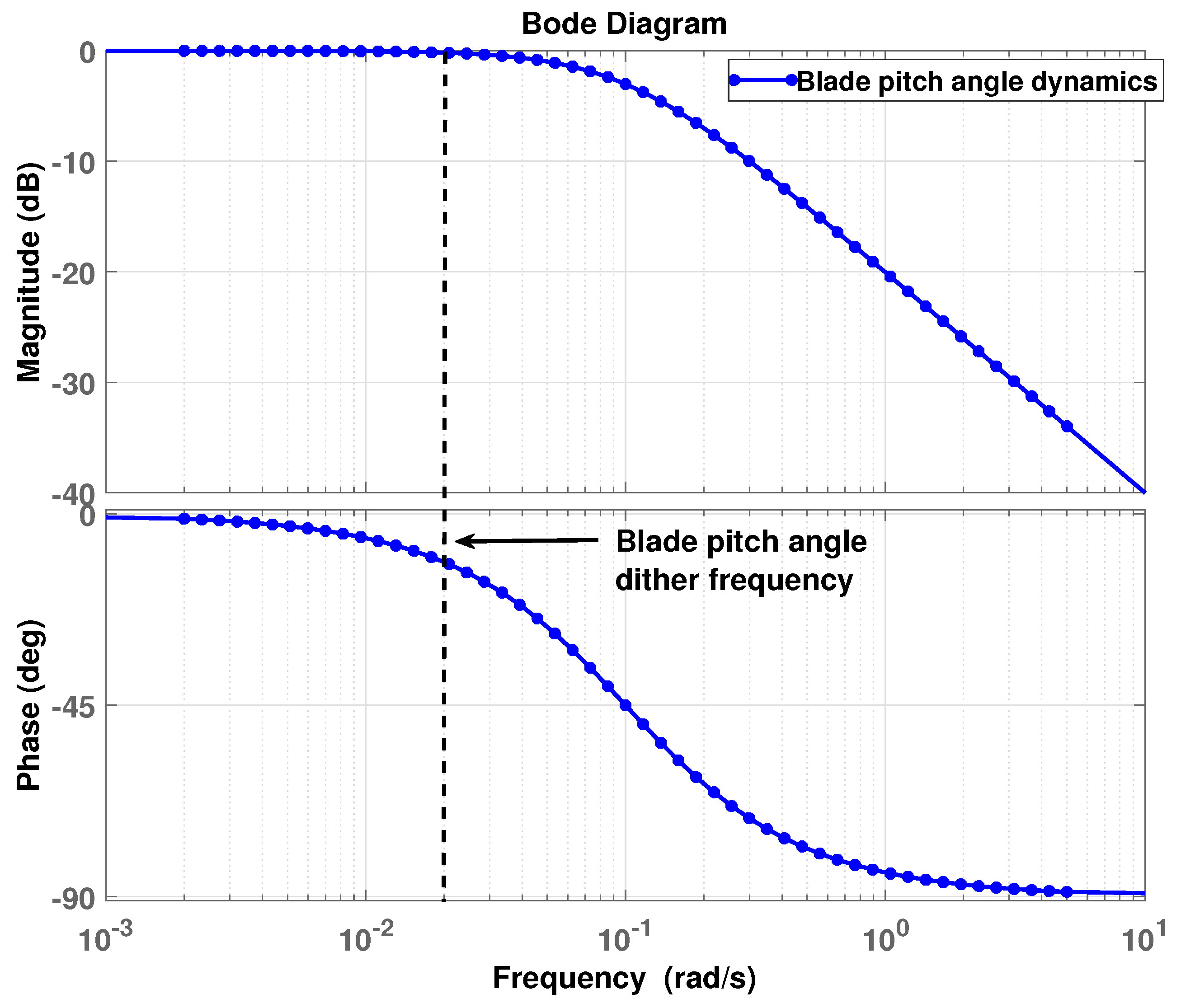
Figure 24.
Bode Plot of input dynamics, and the dither frequency.
Figure 24.
Bode Plot of input dynamics, and the dither frequency.
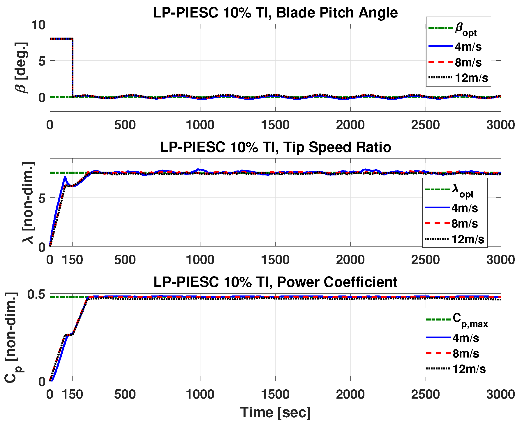
Figure 25.
Performance of LP-PIESC with the parameters shown in
Table 6 and hub-height wind from
Figure 6. Blade pitch angle
(
top), tip speed ratio
(
middle), and estimated power coefficient
(
bottom). The dashed horizontal lines indicate optimal parameters
,
and
. The LP-PIESC is turned on at 150 s.
Figure 26.
Performance of LP-PIESC with the parameters shown in
Table 6 and wind input with 15% TI. Blade pitch angle
(
top), tip speed ratio
(
middle), estimated power coefficient
(
bottom). The dashed horizontal lines indicate optimal parameters
,
and
. The LP-PIESC is turned on at 150 s.
Figure 26.
Performance of LP-PIESC with the parameters shown in
Table 6 and wind input with 15% TI. Blade pitch angle
(
top), tip speed ratio
(
middle), estimated power coefficient
(
bottom). The dashed horizontal lines indicate optimal parameters
,
and
. The LP-PIESC is turned on at 150 s.
Figure 27.
Energy capture comparison: Baseline vs. LP-PIESC. Average energy output with baseline optimal blade pitch angle and LP-PIESC (top), percentage change in energy capture (bottom).
Figure 27.
Energy capture comparison: Baseline vs. LP-PIESC. Average energy output with baseline optimal blade pitch angle and LP-PIESC (top), percentage change in energy capture (bottom).
Figure 28.
Effect of sudden change in blade pitch angle with LP-PIESC on blade-root flap-wise bending moment (BRFW) (
top) and rotor speed (
bottom) compared with the baseline (for hub height wind from
Figure 6).
Figure 28.
Effect of sudden change in blade pitch angle with LP-PIESC on blade-root flap-wise bending moment (BRFW) (
top) and rotor speed (
bottom) compared with the baseline (for hub height wind from
Figure 6).
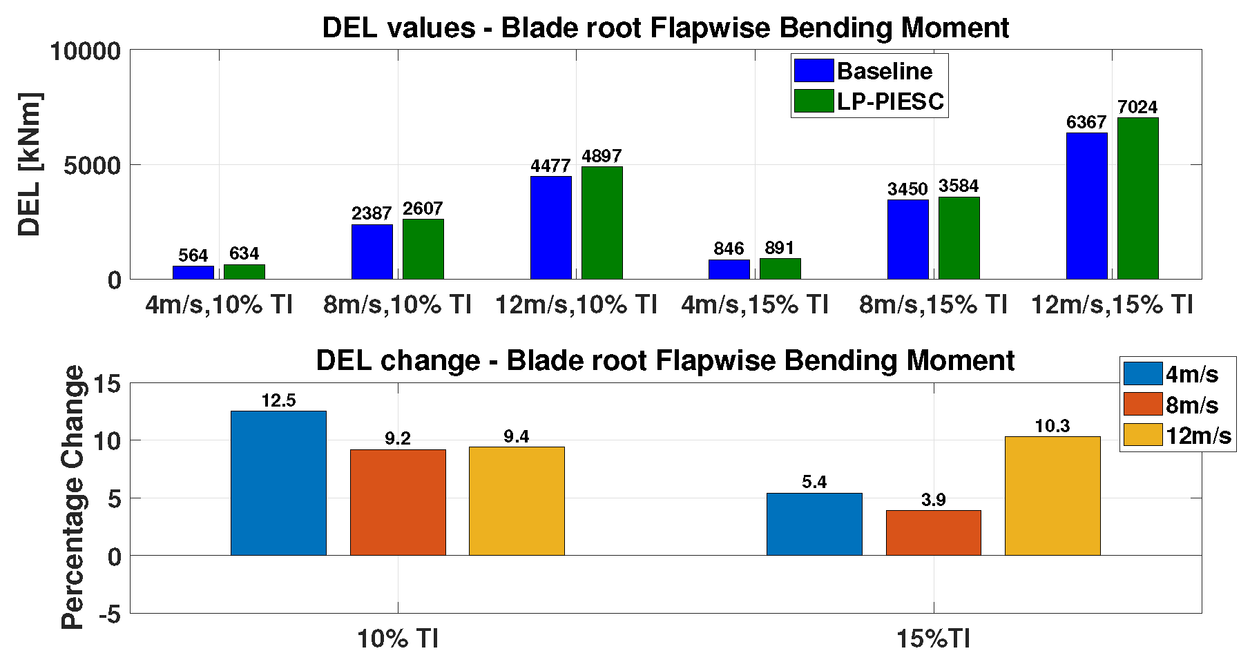
Figure 29.
Blade root flap-wise bending moment comparison: Baseline vs. LP-PIESC. Aggregate DEL values with baseline controller and LP-PIESC (top), percentage change in DEL (bottom) for time series from 150 s to 3000 s.
Figure 29.
Blade root flap-wise bending moment comparison: Baseline vs. LP-PIESC. Aggregate DEL values with baseline controller and LP-PIESC (top), percentage change in DEL (bottom) for time series from 150 s to 3000 s.
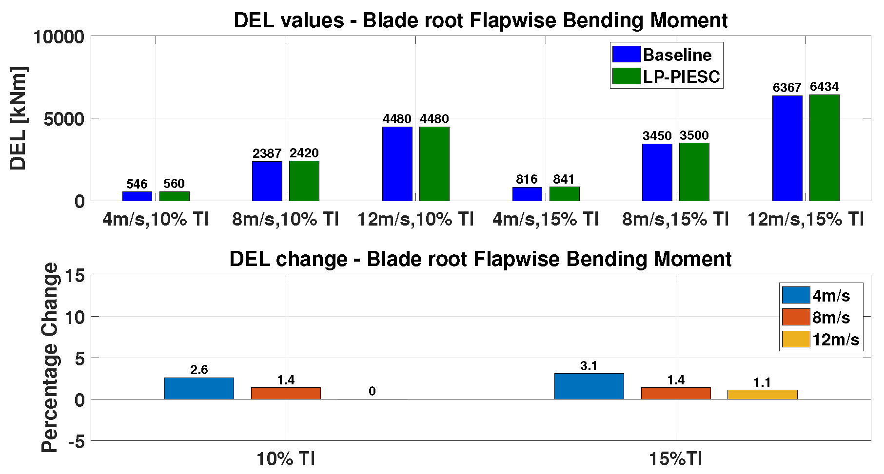
Figure 30.
Blade root flap-wise bending moment comparison: Baseline vs. LP-PIESC. Aggregate DEL values with baseline controller and LP-PIESC (top), percentage change in DEL (bottom) for time series from 300 s to 3000 s.
Figure 30.
Blade root flap-wise bending moment comparison: Baseline vs. LP-PIESC. Aggregate DEL values with baseline controller and LP-PIESC (top), percentage change in DEL (bottom) for time series from 300 s to 3000 s.
Figure 31.
Blade root edge-wise bending moment comparison: Baseline vs. LP-PIESC. Aggregate DEL values with baseline controller and LP-PIESC for time series from 150 s to 3000 s.
Figure 31.
Blade root edge-wise bending moment comparison: Baseline vs. LP-PIESC. Aggregate DEL values with baseline controller and LP-PIESC for time series from 150 s to 3000 s.
Figure 32.
Tower base fore-aft bending moment comparison: Baseline vs. LP-PIESC. Aggregate DEL values with baseline controller and LP-PIESC (top), percentage change in DEL (bottom) for time series from 150 s to 3000 s.
Figure 32.
Tower base fore-aft bending moment comparison: Baseline vs. LP-PIESC. Aggregate DEL values with baseline controller and LP-PIESC (top), percentage change in DEL (bottom) for time series from 150 s to 3000 s.
Figure 33.
Tower base side-side bending moment comparison: Baseline vs. LP-PIESC. Aggregate DEL values with baseline controller and LP-PIESC (top), percentage change in DEL (bottom) for time series from 150 s to 3000 s.
Figure 33.
Tower base side-side bending moment comparison: Baseline vs. LP-PIESC. Aggregate DEL values with baseline controller and LP-PIESC (top), percentage change in DEL (bottom) for time series from 150 s to 3000 s.
Figure 34.
Drivetrain torsion comparison: Baseline vs. LP-PIESC. Aggregate DEL values with baseline controller and LP-PIESC (top), percentage change in DEL (bottom) for time series from 150 s to 3000 s.
Figure 34.
Drivetrain torsion comparison: Baseline vs. LP-PIESC. Aggregate DEL values with baseline controller and LP-PIESC (top), percentage change in DEL (bottom) for time series from 150 s to 3000 s.
Table 1.
Main parameters of NREL 5MW turbine used for algorithm designs.
Table 1.
Main parameters of NREL 5MW turbine used for algorithm designs.
| Description | Value |
|---|
| Rating | 5 MW |
| Rotor radius (R) | 63 m |
| Gear Ratio (N) | 97 |
| Rotor Inertia () | 35,444,067 kg·m2 |
Table 2.
LP-ESC Parameters of NREL 5MW Region 2 controller (see
Figure 1).
Table 2.
LP-ESC Parameters of NREL 5MW Region 2 controller (see
Figure 1).
| Parameter | Torque-Gain LP-ESC |
|---|
| Dither Frequency () | 0.02 rad/s |
| Dither Amplitude (a) | 0.02 (non-dimensional) |
| Cut-off Frequency of LPF | 0.015 rad/s |
| Cut-off Frequency of HPF | 0.018 rad/s |
| Phase Compensation () | 0.36 rad |
| Integrator Gain (k) | 0.001 rad/s |
Table 3.
LP-PIESC Parameters of NREL 5 MW Region 2 controller. See Equations (
6)–(
12).
Table 3.
LP-PIESC Parameters of NREL 5 MW Region 2 controller. See Equations (
6)–(
12).
| Parameter | Torque-Gain LP-PIESC |
|---|
| Dither Frequency () | 0.02 rad/s |
| Dither Amplitude (a) | 0.005 (non-dimensional) |
| 20 rad/s |
| K | 20 rad/s |
| (s/rad)2 |
| 0.000005 s/rad |
| 2.8 (non-dimensional) |
Table 4.
Average energy capture for both LP-ESC and LP-PIESC compared to baseline.
Table 4.
Average energy capture for both LP-ESC and LP-PIESC compared to baseline.
| | Baseline (kWh) | LP-ESC (kWh) | % Change |
| Average Energy Output | 2178.6 | 1869.7 | −14.2 |
| | Baseline (kWh) | LP-PIESC (kWh) | % Change |
| Average Energy Output | 2178.6 | 2171.4 | −0.3 |
Table 5.
Blade, drivetrain, and tower loads considered for analysis with respective natural frequencies.
Table 5.
Blade, drivetrain, and tower loads considered for analysis with respective natural frequencies.
| Load | First Mode Natural Frequency (Hz) |
|---|
| Blade-root flapwise bending moment (BRFW) | 0.5–1 |
| Blade-root edgewise bending moment (BREW)) | 0.9–1.3 |
| Drivetrain torsional moment (DTT) | 1.7 |
| Tower-base fore-aft bending moment (TBFA) | 0.32 |
| Tower-base side-side bending moment (TBSS) | 0.31 |
Table 6.
LP-PIESC Parameters of NREL 5 MW Region 2 blade pitch controller. See Equations (
6)–(
12).
Table 6.
LP-PIESC Parameters of NREL 5 MW Region 2 blade pitch controller. See Equations (
6)–(
12).
| Parameter | Blade-Pitch LP-PIESC |
|---|
| Dither Frequency () | 0.02 rad/s |
| Dither Amplitude (a) | 0.2 deg. |
| 20 rad/s |
| K | 20 rad/s |
| (deg.s/rad)2 |
| 0.000005 deg.2s/rad |
| 2.8 deg.−2 |
Table 7.
Average energy capture for LP-PIESC compared to baseline.
Table 7.
Average energy capture for LP-PIESC compared to baseline.
| | Baseline (kWh) | LP-PIESC (kWh) | % Change |
|---|
| Average Energy Output | 2178.6 | 2172.6 | −0.3 |


