Power Consumption and Effectiveness of Azimuth Stern-Drive (ASD) Tug While Assisting at Ship’s Bow

Abstract

The purpose of this article is to present a methodical approach to increasing the efficiency of a tug with an azimuth stern drive (ASD). The difficulties in the bow-to-bow (as a reverse tractor) operations of an azimuth stern-drive tug, while pulling at the assisted (towed) ship’s bow, are investigated through a parametric study. The authors’ original generic analytical model of a tug in a steady state is utilised. Various design and operation options are also compared, which cover the escort speed, hawser angle, and relative location of the towing point, among others. The latter also means a shift to stern-to-bow operation. The thruster power required and the remaining surplus for executing new alignment (steering) orders are assessed. The study is, thus, aimed at energy savings for the whole operation and, consequently, at long-term harbour-tug-fleet energy effectiveness. The basic output of the present research is the comparison of the behavioural and control patterns of various tug arrangements at a ship’s bow. The results of the study show a slight advantage for a midship winch tug working through her stern for bow operation (stern-to-bow) over the reverse tractor acting bow-to-bow. Comparing various tug designs or operation options is difficult due to complicated tug dynamics and statics patterns under the hawser action. Both relative and absolute towing forces have to be considered (a high relative force may result in a low absolute force, much less than ordered by the pilot), with some geometrical and safety constraints additionally. The practical implementation of the conducted research should cover the guidance and training rendered to tug masters in the scope of the operational limitations of a particular tug and towards the design or acquisition of the tug that is best-suited for a particular harbour operation.

1. Introduction

Large ships (often with one-screw propulsion and without lateral tunnel thrusters) cannot safely enter confined harbours and berth on their own. This is due to their high kinetic energy during an approach speed (roughly about 5 knots), and the limited number and magnitude of the control forces that can be developed by the ship to handle herself in a horizontal plane (3DOFs) and in an arbitrary way (with control over the so-called pivot point). The contemporary research (which is supported by multiple references in the literature, starting from the 1960s) of maritime towing covers the following topics:

(1)

propulsive and hydrodynamic (resistance, manoeuvring, seakeeping) design of tugs, including experimental model tests, CFD computations, and force regression/analytical studies, e.g., [1], or incl. the hook location design, e.g., [2];

(2)

mathematical modelling of tug manoeuvring hydrodynamics (and towing operations) for simulation and/or full-mission simulator implementation, e.g., [3,4];

(3)

choice of the number and power (and type) of tugs for towing assistance, both in the open sea (ocean towing) and a harbour, in terms of operation safety and effectiveness, e.g., [5,6];

(4)

tug roll stability during towline tension;

(5)

ship-to-tug interaction at speed. e.g., [7];

(6)

autonomous tugs and automatic control of tug manoeuvres (e.g., in a simulator environment);

(7)

human-related aspects of tug handling (seamanship), e.g., [8];

(8)

tug GHG emissions, e.g., [9].

There are also a number of successful conferences more or less specifically devoted to tugs, towing, and manoeuvring simulation, and the attached references list is certainly not exhaustive.

This paper is basically situated within the second topic, with some guidance for tug captains, thus relating to the application areas expressed by the last three topics as well. Partly, the present work is an application related follow-up of the authors’ previous developments.

The ship and tug cooperation (and interaction) is a challenging subject, in particular while towing a ship’s bow. Inadequacies of the theory concerning the advantages of a particular tug (or of a particular deployment of a tug’s towing assembly or towing mode) in the ship’s area and all the factors involved, especially those related to the design (the location of the towing point (T) vs. the propeller/thruster (P) installation point and the underwater hull, including the skeg, in terms of shape and size) are matter-of-fact [10,11]. It must be stressed that the present theory is similar to that of an unconventional, highly manoeuvrable cycloidal or azimuth tractor tug application for bow operation (where a towing winch is close to the end of the tug’s stern) vs. a conventional tug (with aft propulsion and a central hook). A lot of discussions/views exist in this context [10,12]. The tug-to-bow operation, to a great extent, inherits the well-known hydrodynamics specific to the operation at a ship’s stern, especially at a high towing (escort) speed [10,11,12,13,14]. In the latter, investigations often go towards the so-called direct and indirect towing (with the augmentation of a tug’s performance via her underwater hull hydrodynamic force).

The azimuth stern-drive (ASD) tug is often called a reverse tractor in the common industry language, especially for bow operation that should be equivalent, at least with some generalisation (e.g., from the tug’s manoeuvrability standpoint), to a tractor tug (with propellers located forward). The basic difference between a reverse tractor tug and a tractor tug comes from the human-centred difficulty while monitoring (visual viewing) and controlling the tug’s movement either in an aft direction (a reverse tractor, bow-to-bow operation) or in a natural forward direction (a tractor tug, stern-to-bow operation at ship’s bow). However, the main issue of the tractor and reverse tractor comparison arises from quite different factors—the mutual location of T (sometimes multiple locations are possible onboard a tug, depending on the design) vs. P. This situation necessitates the future debate and application of a new classification/redefinition of tugs or tug operational modes, since the straight/pure naming as a tractor or reverse tractor is a little confusing.

The bow tug’s design and operation sensitivity to some factors (in terms of efficiency or effectiveness and safety [15]) has been rarely undertaken so far. The presented research is partly inspired by the TNI monograph of Cpt. Hensen [16] and the authors’ previous study on ASD tugs used for bow operation [17] and is aimed at providing some detailed knowledge on certain fundamental aspects. The towed ship–tug hydrodynamic interaction effects were omitted in our study and postponed until future research.

In the following research, the original generic analytical model for tug pull operation statics was utilised [18]. Any type of tug’s hull hydrodynamics and towing assembly arrangement can be input into this model. The towing operation at a ship’s bow is considered in both the bow-to-bow and stern-to-bow configurations, especially with non-zero towing speed taken into account. This method is based on the classical equilibrium of the forces in 3DOF being solved analytically (with numerical support for lookup-table interpolation, where the hull hydrodynamic characteristics are stored), which is very fast, even for spreadsheets. The adopted dimensionless approach serves energy efficiency, and the drift angle domain ensures the uniqueness and completeness of the solution, which are novel features.

Some research centres claim they have developed special software for computing the force (power) exerted by a tug on an assisted ship (and the tug’s control parameters), e.g., [10,19,20,21,22]. However, their published documentation is often insufficient, and the published results (plots, tables, analysis, discussion) are incomplete. In this paper, the capability plots and detailed steering data of a tug are, thus, provided and discussed to enhance the decision support while selecting and operating the particular mode of towing assistance. Although worldwide SI units are critical in various scientific publications and applications, in the maritime industry, especially in ship structural design and operation, and seamanship, the unit of the ton (or precisely but more rarely ton-force, t) is still commonly used for force expression. Partly, a similar situation exists with respect to the knot as a unit of speed or velocity. Sometimes, to provide direct conversion if needed, double (or parallel) units are used. Therefore, the units of ton and knot ([t], [kn]) are used throughout this paper.

The paper presents problems concerning the difficulties in the bow-to-bow operations of an ASD tug, while pulling at the assisted ship’s bow. Its contents are structured as follows:

(a)

problem formulation, materials and methods including a literature review, a mathematical model of an exemplary tug, and simulation cases, in Section 2;

(b)

results of a parametric study of the tug’s towing point vs. her propeller location, in Section 3;

(c)

discussion, in Section 4;

(d)

conclusions and further research plans, in Section 5;

(e)

plots comparing the reference cases to other hydrodynamics and supplementary cases, in the appendices.

2. Problem Formulation, Materials, and Methods

The description (with appropriate discussion) of the harbour tug model, physics, and derived solution for tug’s static equilibrium is presented in Section 2.1. Furthermore, the computational scenarios, based on the most representative, extreme (providing the deepest insight and knowledge) cases of T vs. P location are presented in Section 2.2.

2.1. Case Study Tug and Mathematical Model of Static Equilibrium

The investigated tug of generic type and environmental parameters were, for consistency with the previous research conducted by the authors [14,17,18]:

• length between perpendiculars (as a reference length), (L) 30.5 m;
• draught (as a reference draught), (T_ref) 5 m;
• water density (ρ), 1000 kg/m³.

The tug described above is a typical harbour one and as such can accommodate various engine powers (bollard pull) within the ship size as presented, e.g., in [23]. The tug length and draught are used hereafter to determine the lateral underwater area (by convention being the product LT_ref) necessary for computing hull (H) hydrodynamic forces on a tug due to her movement through water. Knowing the basics of similitude in ship hydrodynamics (where, e.g., the applied dimensionless coefficients are strictly dependent on the reference area used in order to obtain the appropriate/measured force magnitude), one can freely and easily extrapolate or fit all the following research output to their needs.

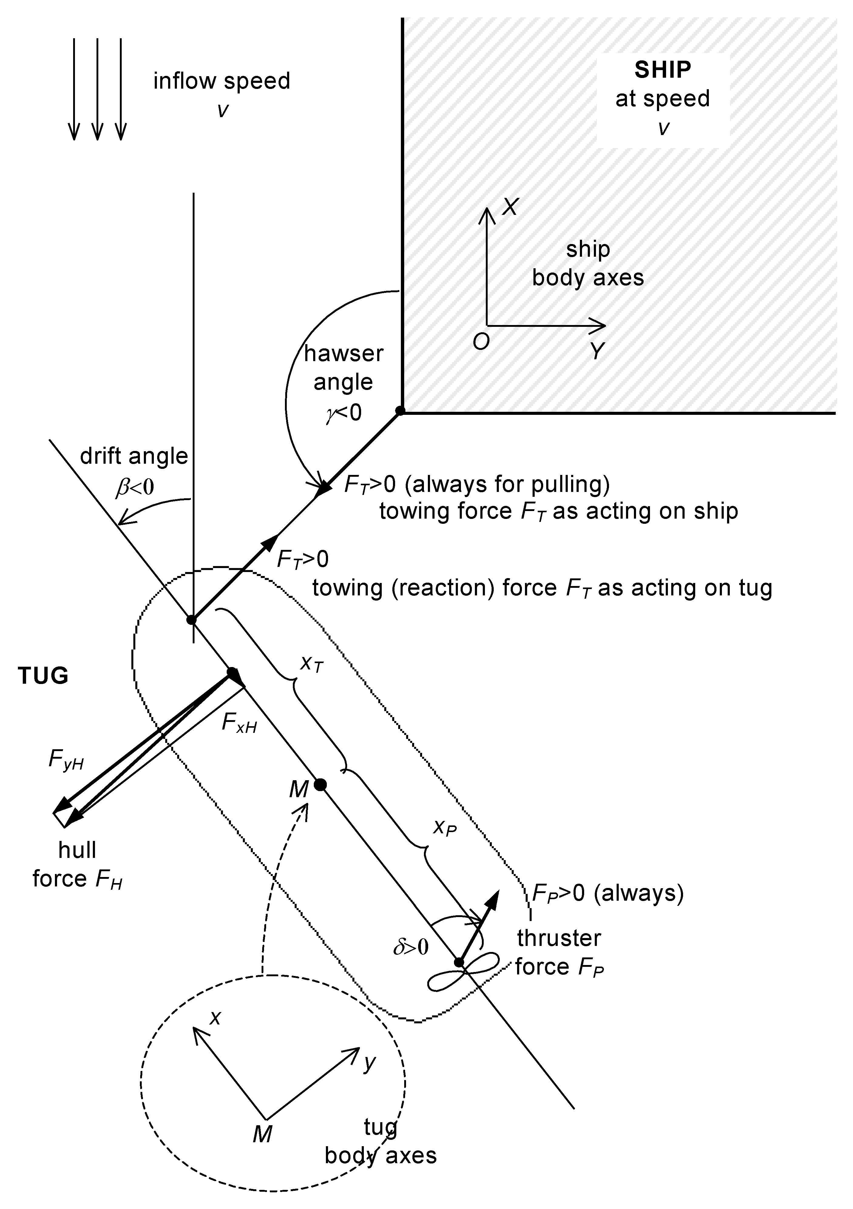
The reference frame used to study the dynamics/statics of a tug (the most important item in our study of the two-body system—small tug and large ship) is that of the tug itself (see Figure 1). The steady-state condition can be, hence, written as follows:

$$\{\begin{array}{ccc}{F}_{xH}+F_{xP}+F_{xT}& =& 0\\ F_{yH}+F_{yP}+F_{yT}& =& 0\\ M_{zH}+M_{zP}+M_{zT}& =& 0\end{array}$$

(1)

where F_x, F_y—longitudinal and lateral force, and M_z—yaw moment.

$$\left[\begin{array}{c}{F}_{xH}\\ F_{yH}\\ M_{zH}\end{array}\right]=0.5\rho L{T}_{ref}{v}^2\left[\begin{array}{c}{c}_{fxh}\left(\beta \right)\\ c_{fyh}\left(\beta \right)\\ L{c}_{mzh}\left(\beta \right)\end{array}\right]$$

(2)

where c_fxh, c_fyh, c_mxh—hull hydrodynamic dimensionless coefficients as functions of drift angle β in the range (−180°, +180°〉 to obtain the full general solution (the additional yaw velocity contribution disappears in a steady state), and v—towing (escort) speed.

$$\left[\begin{array}{c}{F}_{xP}\\ F_{yP}\\ M_{zP}\end{array}\right]=F_P\left[\begin{array}{c}cos\delta \\ sin\delta \\ {x^{\prime }}_P·L·sin\delta \end{array}\right]$$

(3)

where β—propeller/thruster angle (the angle of thrust force) in the range (−180°, +180°〉), and x′_P—propeller/thruster dimensionless location (in tug’s length unit, typically ≈ −0.5 for stern-drive tug, but this study also considers the other extreme case, −0.3, which may reflect, by symmetry and similarity, the performance of forward-drive (azimuth or Voith-Schneider) tractor tug. Hereafter, because a tug usually incorporates dual/twin azimuth propulsors, they are treated as a single propulsor of double force or power, as depicted by F_P (that is positive definite, by default), thus of their parallel/combined action.

$$\left[\begin{array}{c}{F}_{xT}\\ F_{yT}\\ M_{zT}\end{array}\right]=-F_T\left[\begin{array}{c}cos\left(\gamma -\beta \right)\\ sin\left(\gamma -\beta \right)\\ {x^{\prime }}_T·L·sin\left(\gamma -\beta \right)\end{array}\right]$$

(4)

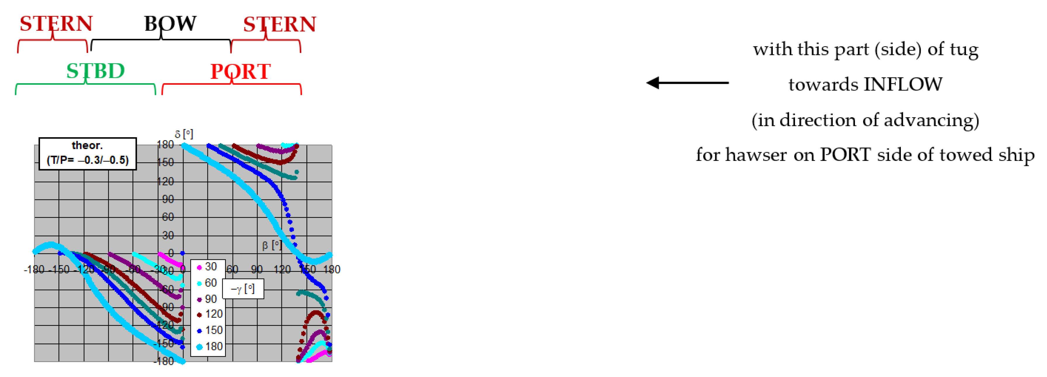
where γ—hawser (towing line) angle in the range (−180°, +0°) we assume the operation on port side of the assisted ship (6 to 12 o’clock), and x′_T—towing point (hook/winch/fairlead) location (in tug’s length unit, typically ≈ +0.5 for stern-drive tug, acting through her bow as reverse tractor, but this study also considers other intermediate cases). The starboard-side operation is to be easily derived by symmetry rules.

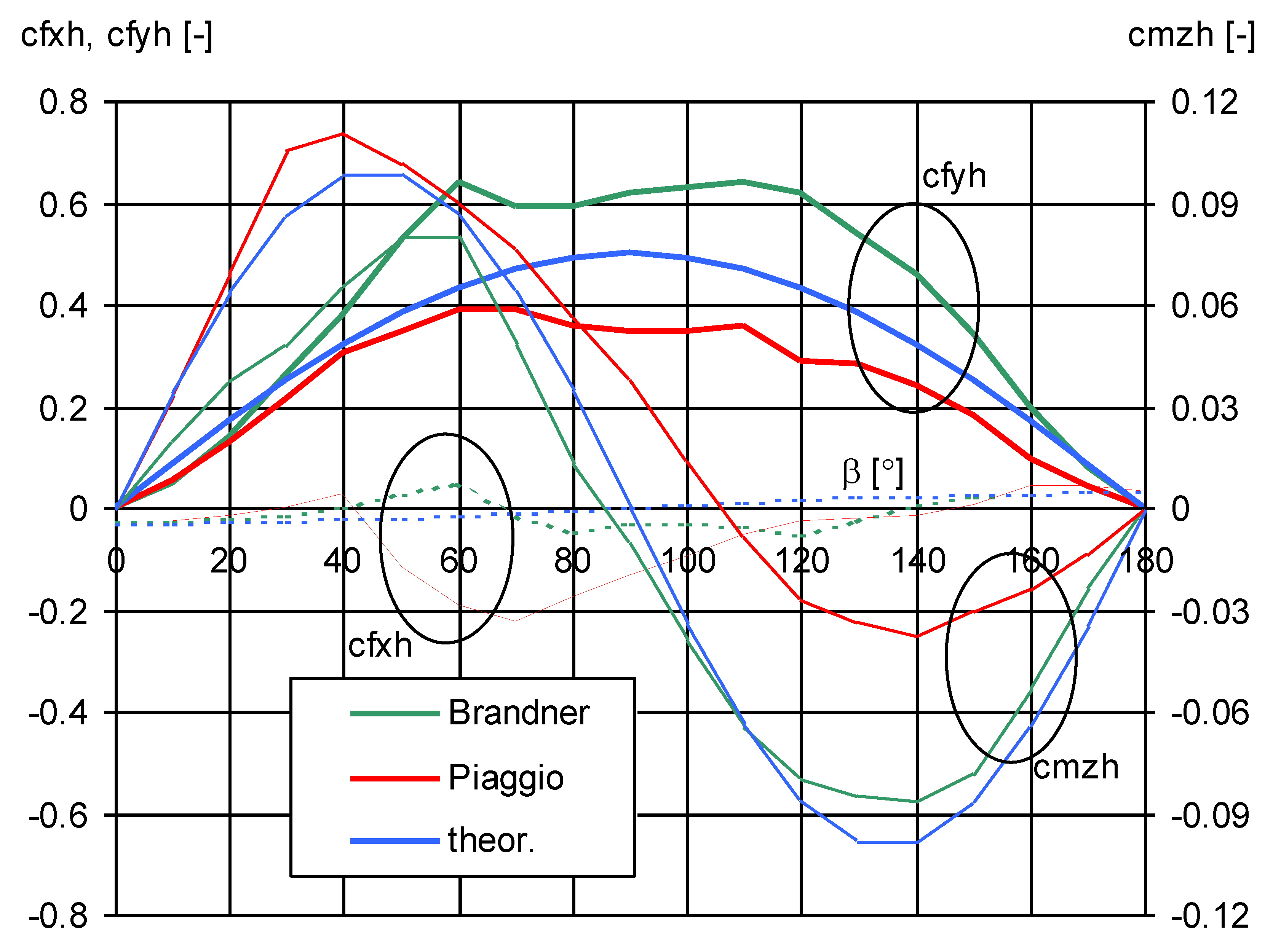
For consistency, the theoretical hydrodynamic data are the same as in [9]:

$$\{\begin{array}{ccc}{c}_{fxh}\left(\beta \right)& =& -0.03cos\beta \\ c_{fyh}\left(\beta \right)& =& +0.5sin\beta \\ c_{mzh}\left(\beta \right)& =& +0.1sin2\beta \end{array}$$

(5)

which are used to represent the basic, reference case (‘theor.’). However, to examine the validation of this theoretical case and possible actual deviations from it, our sensitivity study covers also tug response for other published hydrodynamic model data [24,25] (only for the reference T and P locations, see below), hereafter called ‘Brandner’ and ‘Piaggio’, accordingly. These are jointly presented in Figure 2. ‘Brandner’ case suits rather well the theoretical case, while ‘Piaggio’ deviates more. Both tugs differ in their underwater design.

In order to provide the final solution/algorithm in the most universal/dimensionless and compact form (e.g., denominated in propeller force) based on [18], let us define the ratios:

$${c^{\prime }}_{fxh}\left(\beta \right)=\frac{c_{fxh}\left(\beta \right)}{c_{fyh}\left(\beta \right)},{c^{\prime }}_{mzh}\left(\beta \right)=\frac{c_{mzh}\left(\beta \right)}{c_{fyh}\left(\beta \right)}$$

(6)

$${F^{\prime }}_T=\frac{F_T}{F_P},{F^{\prime }}_H=\frac{F_{yH}}{F_P}$$

(7)

The solution, for a given towing speed v, now constitutes the following form of four consecutive (sequential) steps:

$${\tan }^{-1}\delta =\frac{-{x^{\prime }}_P+{c^{\prime }}_{mzh}\left(\beta \right)}{{x^{\prime }}_T-{c^{\prime }}_{mzh}\left(\beta \right)}\left[-{\tan }^{-1}\left(\gamma -\beta \right)+{c^{\prime }}_{fxh}\left(\beta \right)\right]+{c^{\prime }}_{fxh}\left(\beta \right)$$

(8)

$${F^{\prime }}_T=\frac{sin\delta }{sin\left(\gamma -\beta \right)}·\frac{-{x^{\prime }}_P+{c^{\prime }}_{mzh}\left(\beta \right)}{-{x^{\prime }}_T+{c^{\prime }}_{mzh}\left(\beta \right)}$$

(9)

$${F^{\prime }}_H=-sin\delta +{F^{\prime }}_{T}sin\left(\gamma -\beta \right)$$

(10)

$$F_P=\frac{0.5\rho L{T}_{ref}{v}^2{c}_{fyh}\left(\beta \right)}{{F^{\prime }}_H}$$

(11)

If we assume a constant hawser angle γ ordered by the pilot, of the 5 control (unknown) variables—β, δ, F′_T, F_P, and v—only the first three provide a unique solution, when this solution is being sought in β domain. Therefore, the latter domain is the basis for this study. The drift angle is the independent variable and is to be considered in full range (−180°, +180°). Although we assumed the hawser on port side of the towed ship, the tug may, at least in theory and our solution, face her port (positive β) or starboard side (negative β) with the water inflow. The absolute towing force F_P (in tons) and v are mutually related, according to (11), based on previous variables through (10). Thus, F_P can be established if one knows v and vice versa.

There is necessity to reduce the possible mathematical solutions of the equation system (8)–(11), to acquire the valid physics. Thus, only those solutions where F′_T > 0 should be preserved (the hawser is being tensioned instead of compressed; in other words, it works only in one, the right, direction, thus unlike a spring acting in both directions). This can be accomplished by modifying δ from (8) and adding ±180° (as tan⁻¹ nominally returns values from −90° to −90°), to keep δ in the original range (see explanation for (3)). Moreover, in view of hydrodynamics, we have to disregard those solutions that do not satisfy the condition of equal signs (positive or negative) for both and F′_H and β.

The full algorithm, which is flexible enough to easily accommodate other hydrodynamic input data and is ready for future improvements, was implemented in MS Excel spreadsheet. Code/numerical verification, the physical validation, and output presentation were automated.

2.2. Simulation/Computational Cases

The following cases of (x′_T, x′_P) are considered in the steady-state solution to obtain the full-range behavioural pattern for astern-drive (azimuth) tug:

• main cases: (+0.5, −0.5) (‘REF’); (0, −0.5); (−0.3, −0.5);
• supplementary cases: (+0.3, −0.5); (+0.4, −0.3).

Two speeds, typical for harbour manoeuvres, of 4 and 6 knots (ca. 2 and 3 m/s) were selected to show the effective pull required and, indirectly, the margin to the tug power (for, e.g., new tug alignment/manoeuvring orders).

The main directions γ (every one hour, on port side of the towed ship, as described before) from 0° (12 o’clock) up to −180° (6 o’clock) were used. However, additional values of −45° and −135° were also included in our investigations but are not shown for plot resolution purposes; besides, they do not exhibit a specific behaviour among the surrounding main values. For γ = 0° (the tug at 12 o’clock), the cases of β ≠ 0° do not return a valid physical solution. On the other hand, the trivial case of β = 0°, although physically justified, is numerically ill-posed, as in deriving our solution we use the function c′_fxh (β)—see (6)—that assumes numerically inconvenient ±∞ for β = 0° and terminates the computations. This is why the case γ = 0° disappears in our next figures. The only exception is the supplementary case (+0.4, −0.3), where such a non-trivial solution really exists.

Considering the design and operational practice, e.g., [10,11], for harbour tugs, the above simulation choices seem to represent, in a simple way, the wide variety of possible solutions to towing assembly (devices) on a tug. The first (‘REF’) is typical for reverse tractor operation, with a hawser leaving the tug’s forward centre lead (at bulwark) or close to it (as more or less directly running out of the bow winch). However, to investigate the impact of a potential higher offset in the bow winch, the extra and rather extreme case of (+0.3, −0.5) for (x′_T, x′_P) is also included in the study.

The other supplementary case (+0.4, −0.3) that is used can reflect the normal situation for tractor tugs (with forward-located propellers, mostly of Voith Schneider type, see [23], but not always, under the bow, at certain distance from the forward perpendicular). The tractor tug, with some generalisation (omitting less important details), can be essentially looked at as a reversed tractor. As for Voith Schneider tug, see, e.g., [10] (derived from the official Voith company’s booklets/leaflets), the towing point is ca. 10–20% L from the stern, which is why it was assumed to be +0.4 above, for our sensitivity analysis.

In view of the preceding two paragraphs, the ASD tug was considered as a generic omnidirectional tug (able to provide arbitrary thrust in full 360° range), i.e., independent of the principle of operation for the propeller itself. Although such a propeller is nominally located in the aft end of δ a tug (according to the word ‘stern’ in the ‘ASD’ name), our rather general study was not bound by this fact. The name ASD was used in the most common, usual, daily, and general meaning, partly contrary to [10], where the name ASD was reserved only for a multi-tug that can pull both over her bow and stern (over stern, like a conventional tug, with aft-located fixed shaft propellers and passive rudders), dependent on a pilot or tug master’s decision. However, the presented numerical simulation is close to this ‘multi-purpose’ ASD tug meaning, as adopted in [10]. This is why the study covered a pulling assistance on the midship (central) hook/winch—case ‘(0, −0.5)’—or a towing on a winch (hook/staple/fairlead) mounted more towards the tug’s stern—case ‘(−0.3, −0.5)’. The latter is also partly equivalent to the use of staple in a conventional tug for ship-stern operation, as shifting the towing point more aft from the midship location reduces the risk of girting.

For harbour tugs (quite different from escort tugs in unsheltered waters assisting at high towing speed, although with the same physics), dependent upon many factors, the bollard pull BP (and, correspondingly, the engine power installed, which comes roughly almost linearly with BP—refer to [10,23]) is between ca. 20 and 80 t. One should also be reminded that the F_P force (computed in the course of our study), as absorbed by a tug, is the effective force provided by a tug at certain towing speed that is little different from BP (rated for zero speed), particularly if we assume a limiting value for this force. In our study and presentation of results, in view of chart resolution, the limit of 50 t for F_P was applied to reveal the tug’s fundamental performance.

3. Results of Parametric Study

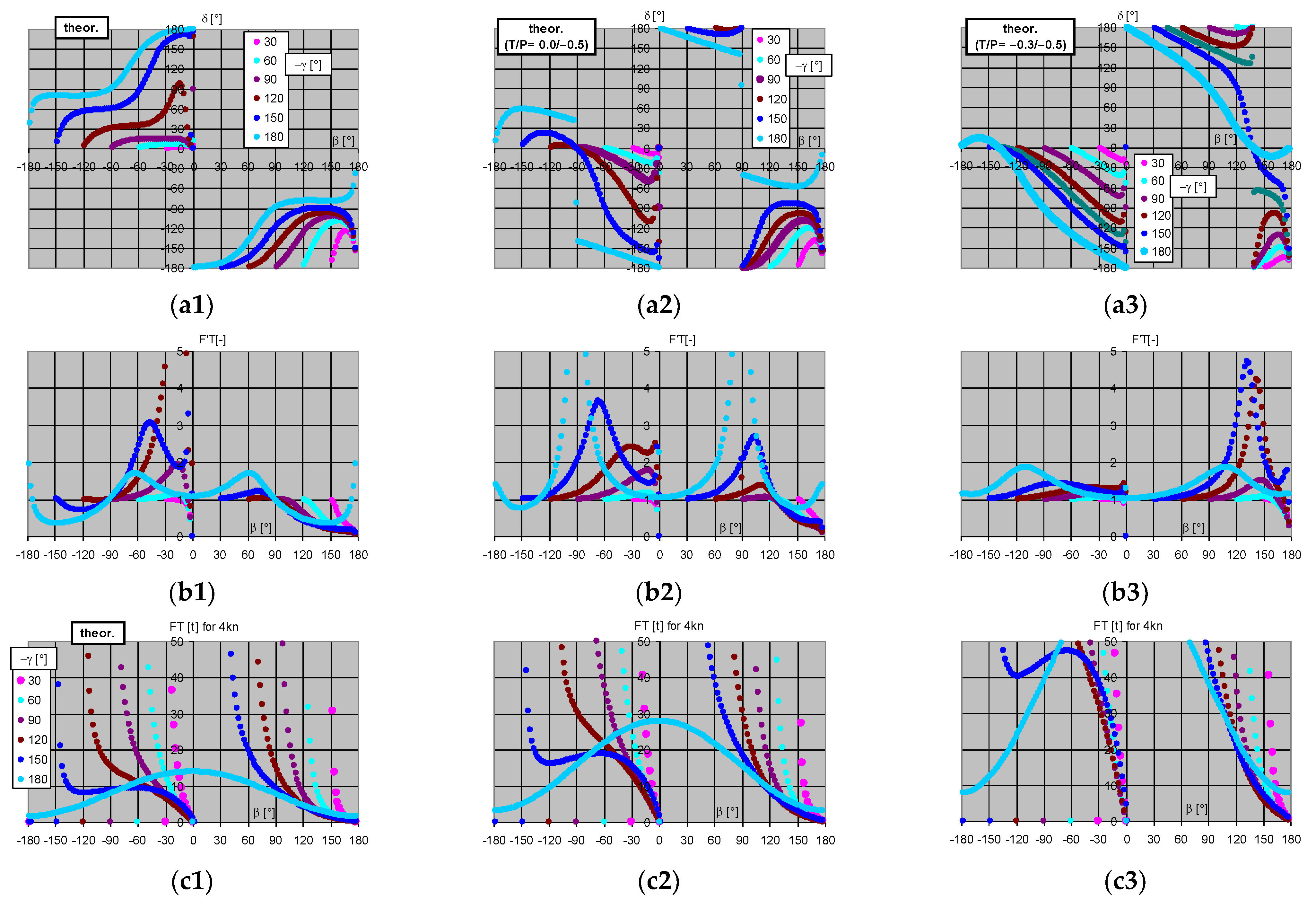
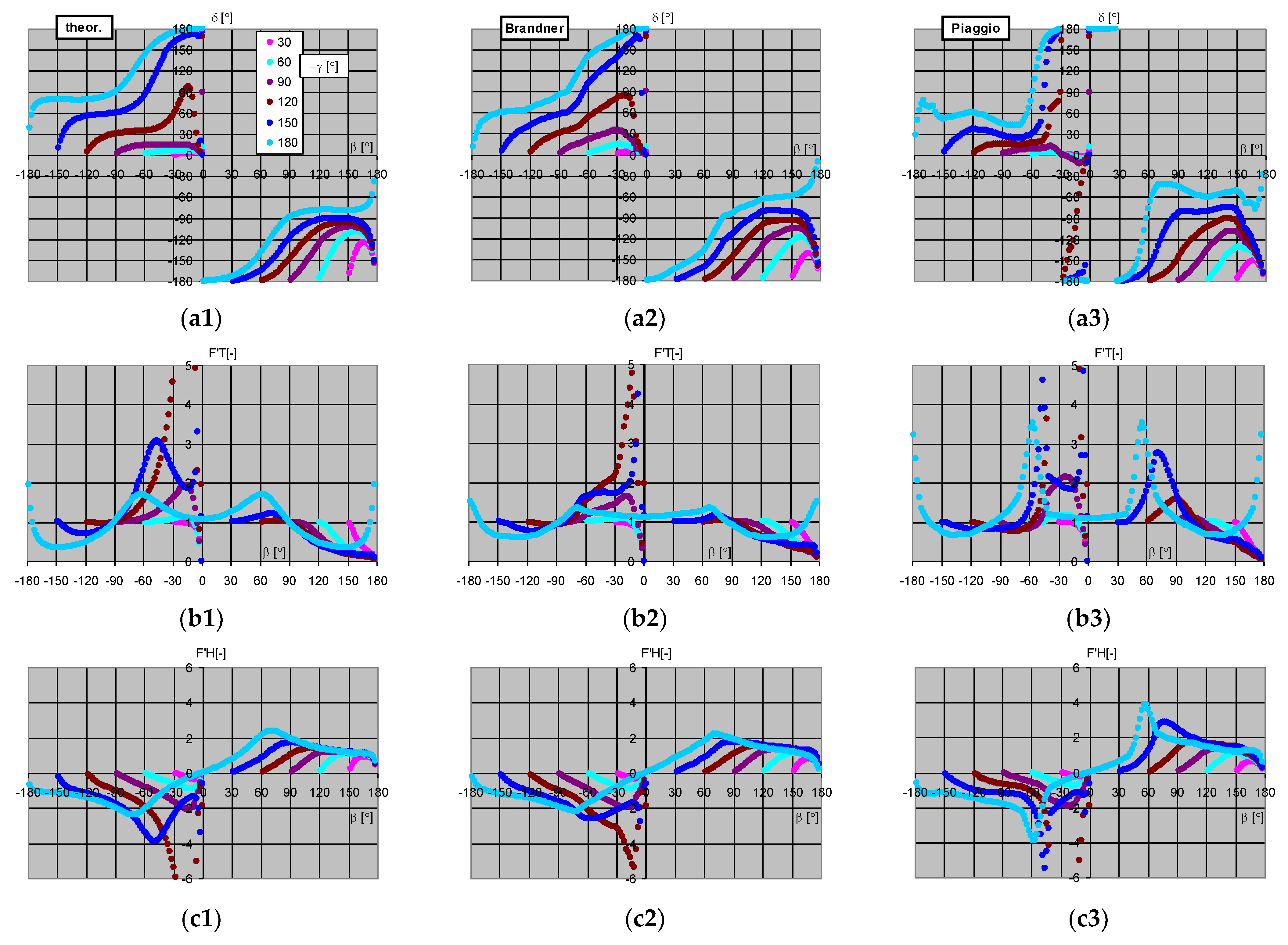
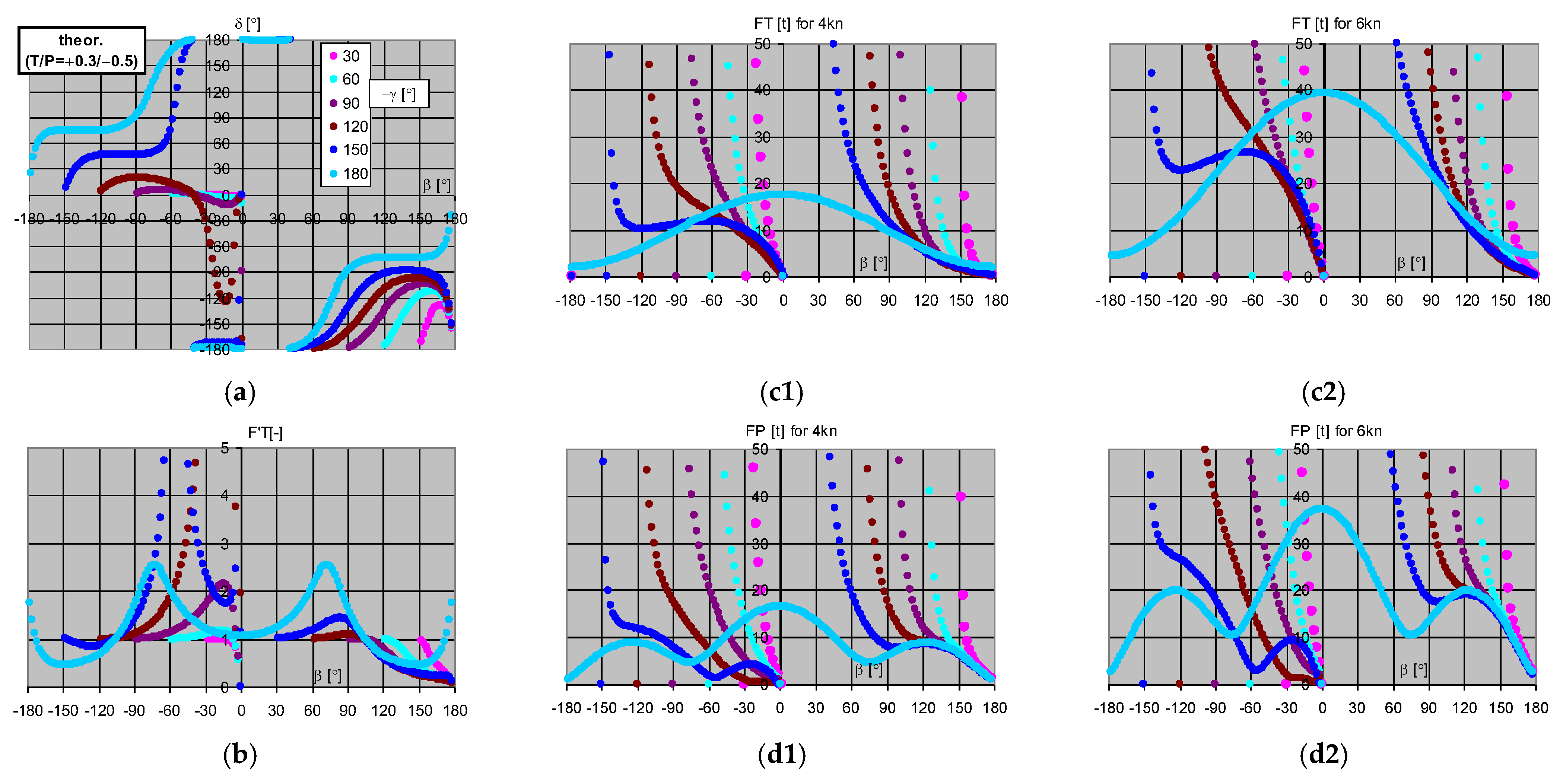
The output data in a compact form for the three main cases of the T (towing point) vs. P (propeller) locations, but with respect to the theoretic hydrodynamics of (5), are displayed in Figure 3 and Figure 4. The rows of subfigures in Figure 3 mean different variables and the columns present different variants of T and P.

Figure 4 directly shows, based on Figure 3(a3), how to interpret the drift angle (and the possible tug’s alignment to water inflow). All such detailed figures are rarely published, so this provides a full insight into the phenomena and tug performance, optimising her power/energy absorption through special operational decisions and the actions that are available at hand (which are not always directly considered during the tug design stage).

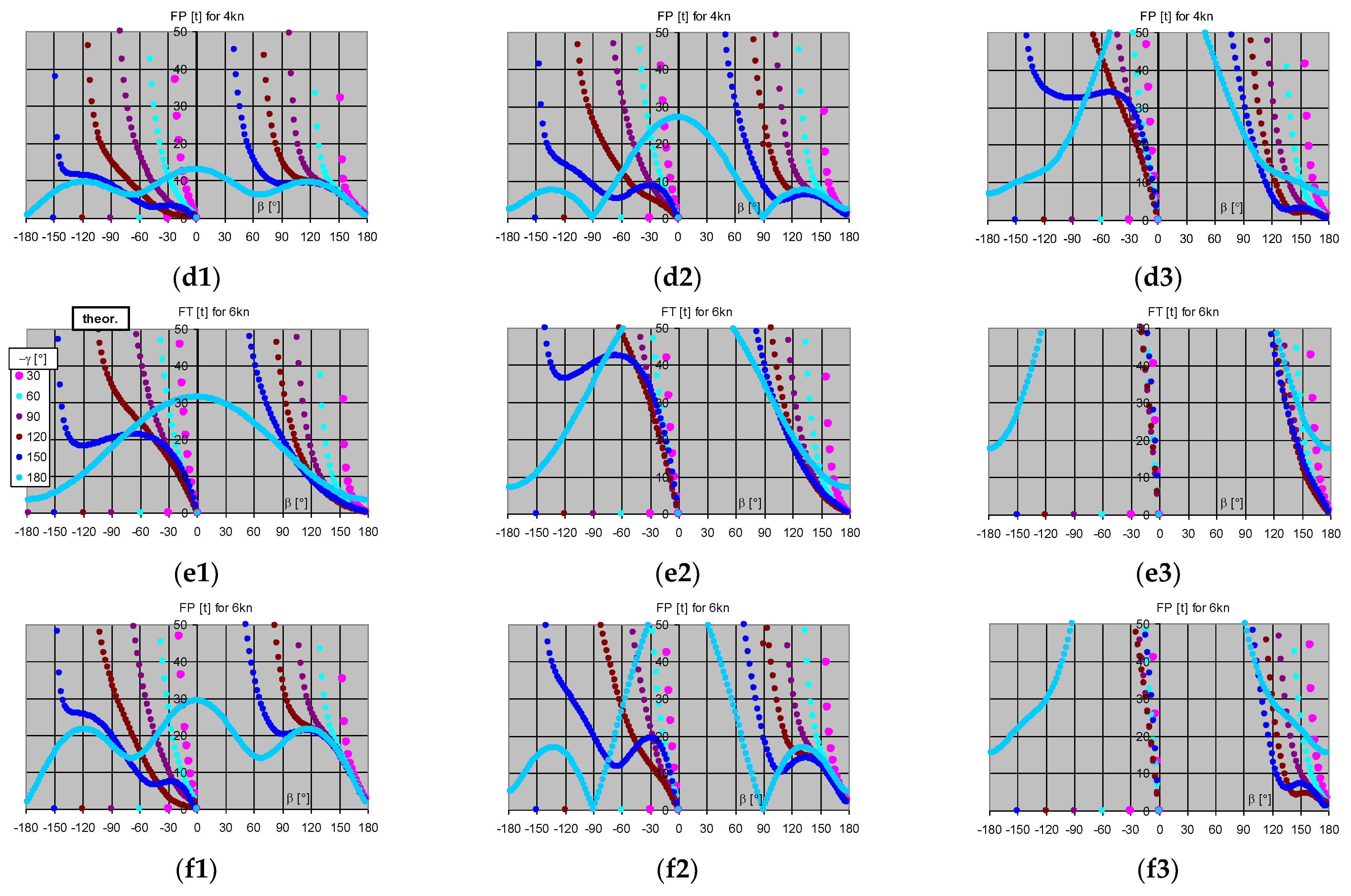
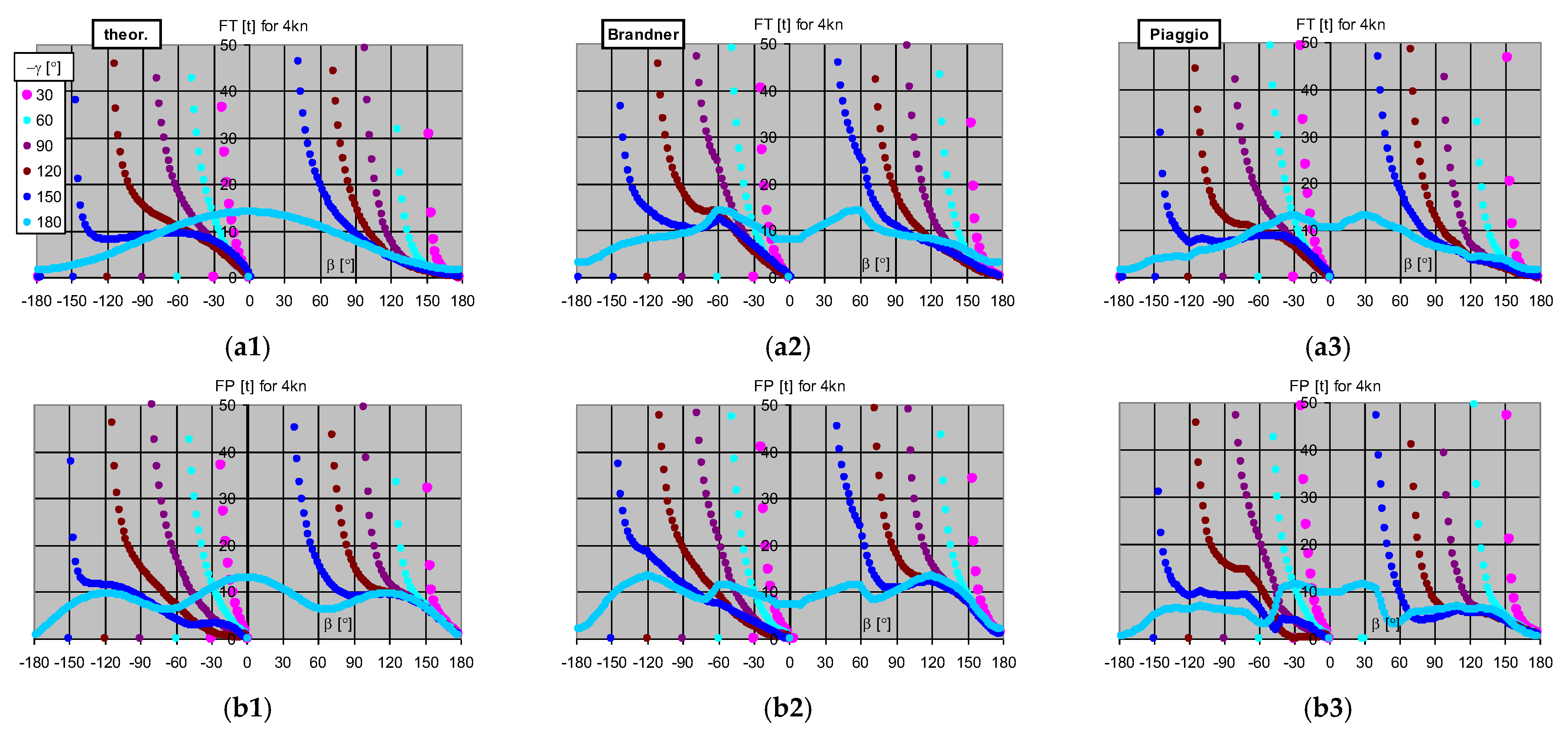
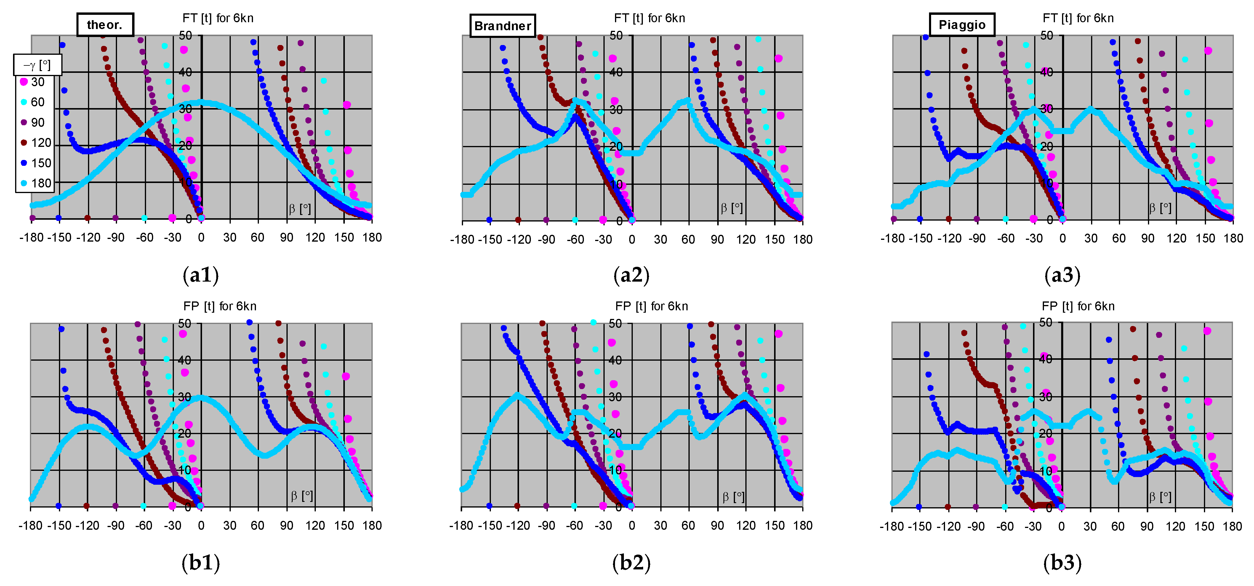
The comparison of the reference case ‘T/P’ = ‘+0.5/−0.5’ to other hydrodynamics (see Figure 2) is provided in the Appendix A Figure A1 (propeller angle δ, effective dimensionless/relative towing force F′_T, dimensionless hull lateral force F′_H), Figure A2 (absolute, i.e., expressed in t, towing and propeller forces, F_T and F_P, for a towing speed of 4 knots), and Figure A3 (same as before, but at 6 knots). The rows of subfigures of Figure A1, Figure A2 and Figure A3 in Appendix A mean different variables and the columns present different sources of hydrodynamic data.

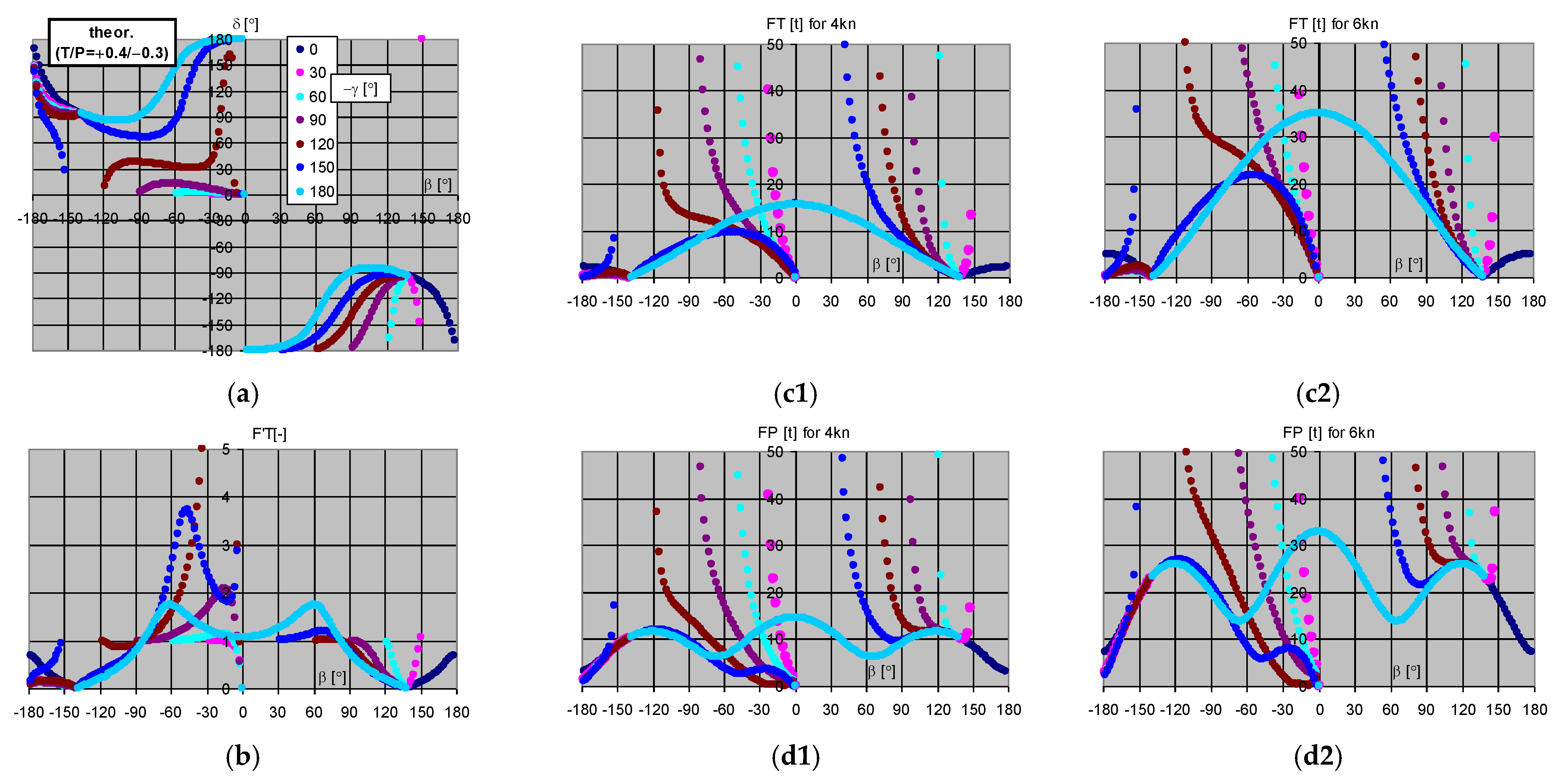
The supplementary cases of T vs. P, for the theoretic hydrodynamics, are also illustrated in the Appendix A, although with a brief presentation: Figure A4 for case ‘T/P’ = ‘+0.3/−0.5’ and Figure A5 for case ‘T/P’ = ‘+0.4/−0.3’ (as aforementioned, the only case with a hawser angle of zero (γ = 0°) included).

The effective operation happens if F′_T > 1; in general, more is better, e.g., for a proper drift angle choice. However, such options (with a significant augmentation of the towing force over that developed by the propeller itself, e.g., F′_T = 1.2 means that we have only a 20% yield) are sometimes not available due to the physics involved. Moreover, a magnitude much less than 1 should be avoided as far as possible (since, paradoxically, the towing force is less than the propeller force, thus of low efficiency). The pilot always orders the best command—in terms of force and angle—for a piloted ship in the current nautical and weather situation and in view of the manoeuvring/movement goals. Then, it is on the tug master how to achieve this in a final steady-state condition (since the work of a tug usually lasts for some longer/shorter time) and in a transient phase (when changing the command, especially in the form of a new towing angle), taking into account the tug’s safety, operability (effectiveness), and available power (propeller force) reserve. For example, if a tug is designed for (maximum) BP = 50 t, then she would experience a certain difficulty if forced to render assistance at a high speed (e.g., 6 knots), if the absolute towing force F_P read off our plots is close to those 50 t.

4. Discussion

By examining Figure A1, Figure A2 and Figure A3 in the Appendix A, one may conclude that the theoretic case is close to the ‘Brandner’ case, as should be clear from the aforementioned direct comparison of hull hydrodynamics (Figure 2). Only some minor, quantitative differences exist in the provided tug’s control and effectiveness variables (steady-state solutions), thus showing a rather low sensitivity in the tug’s performance. Major differences, including those that re qualitative, on the other hand, can be noticed with respect to the ‘Piaggio’ case. However, partly due to this research’s main focus (the impact of a tug’s employment mode, i.e., expressed by the towing point/winch and propeller location), this type of tug (hull hydrodynamics) is postponed to the future full mission simulator tests in dynamic scenarios using a tug master, in order to evaluate the advantages (or disadvantages) during real-time manoeuvring, before making a deeper analytical study in a steady state.

Returning to the main subject, i.e., the study and comparison of the operation effectiveness at a ship’s bow via a tug’s bow winch/lead (‘T/P’ = ‘+0.5/−0.5’), midship (central) winch/lead/hook (‘T/P’ = ‘0.0/−0.5’), and winch/lead/hook moved aft (or other compatible device) (‘T/P’ = ‘−0.3/−0.5’)—first of all, one must notice that some points/segments of the resultant plots are not available. For example, in Figure 3, columns (1) to (3), the first tug is not technically able to sail with drift angle β around 0° (i.e., bow-first, see Figure 4, even though this is a rare case for this tug) at a hawser angle γ close to −180°. A similar situation happens for the second tug (with a central hook, most frequently advancing just bow-first), which, on the other hand, is disabled for rare drift angles ±30° around 180° (stern-first operation). The third tug (intermediate aft wind), which partly inherits the mentioned drawbacks of the second tug, would also experience a collision/contact risk (especially if deployed on a short hawser close to the hull of a towed ship) in an area of high towing-force efficiency (F′_T >> 1), i.e., for a hawser angle ca. −120° to −150° and positive drift around 120° to 150° (Figure 3(b3)). This is a shortcoming of the simple mathematical model and algorithm used, where we do not consider the geometrical restraints for the hawser, as might run across a tug’s deck superstructures and fittings. This calls for some better methodical approach in the next investigations on tug performance with different winch locations. Until now, there has been no well-established standard in performing similar studies, and, thus, these are the first methodical steps in this area.

One must also observe that relative/dimensionless towing force F′_T (higher is better) is a good indicator of efficiency. If we have a look at Figure 3, subfigures (b1/F′_T), and, as an example, (e1/F_T) – (f1/F_P), corresponding to 6 knots, then we know that for practical hawser angles from −90° to −150° and a negative drift in the range from −60° to somewhere near −15°, we acquire a good towing force F_T with very little effort from the propeller (F_P) (the efficiency in terms of F′_T is much more than 1). However, if in those conditions one would set a limit to the low drift angle (abt. −30°), then the maximum towing force F_T in the steady state is only 20t. If one wants to increase this force, they have to increase the drift magnitude (within a negative range), even to set the tug aside towards the inflow (which is difficult to control) and, hence, lower the efficiency. That is why both indicators—relative and absolute towing force—are always worth being considered in parallel.

On the other hand, one should also be interested in much lower (but positive) efficiency, 20 ÷ 30% (F′_T = 1.2 ÷ 1.3), and avoid excessive periods of operating at a complete loss of efficiency (F′_T << 1), if this is the need from the pilot’s point of view and their manoeuvring/steering orders). For example, for a hawser angle between −30° and −60° and the first bow winch tug (Figure 3(b1,e1,f1)), one has to take care to run stern first with a drift angle of −150° and −120° accordingly (and have F′_T≈1), which is equivalent to having a tug’s centre plane in line with the hawser; otherwise, we will be at a low efficiency.

In the case of the second, central hook tug (Figure 3(e2,f2)) and 6 knots, within a negative drift angle, and independent of any hawser angle, a remarkable feature is that the tug keeps an absolute towing force (varying linearly with the drift angle—the higher the drift magnitude is, the higher the towing force is). The propeller’s absolute force and, thus, the relative towing force (>>1), assumes a much more complicated pattern in this instance.

The third, intermediate aft winch tug (Figure 3(e3,f3)), at 6 knots, exhibits a very simple behavioural pattern—both the towing and propeller absolute forces vary linearly with the drift angle (in its negative range, up to −30°), independent of the hawser angle at all. In this situation, the constant medium (c.a. 25%) yield is achieved for the towing force (F′_T ≈ 1.25).

To summarise, comparing various tug design or operation options is difficult due to the complicated tug dynamics (statics) patterns under the hawser action, which involve multiple dimensions (parameters or factors). Both relative and absolute towing forces have to be considered (high relative force—high ‘efficiency’—may produce a low absolute force, much less than ordered by the pilot—thus of slim ‘effectiveness’), additionally with some geometrical and safety constraints. Generally—the better the efficiency is, the worse the effectiveness is at a significant towing speed. Both a low to medium (which are also useful in a lot of situations) as well as a high towing force yield must be examined, which partly depend on an assisted ship’s speed. The provided charts show some essential potential for developing a theory for tug design and operation optimisation. Controlling drift angle β is important for keeping towing force efficiency. In general, a 30–60° hawser order is without any gain (F′_T ≈ 1) for each tug. For the other directions, there are more differences in the gain between each tug and, thus, in the margin for executing new orders.

Roughly speaking, in view of only what is mentioned above, the midship winch tug seems to be the best solution for towed ship-bow operation (as a good compromise between all the merits and drawbacks, in terms of hydrodynamics and control). This last statement needs to be validated in a more systematic way in the future, by also including other factors that are omitted in the present research (such as, e.g., the problems of excessive list and the risk of capsizing/girting at a high towing speed, when a midship winch tug’s control and safety can be lost, although this is not as serious for ASD tugs when compared to conventional tugs). As a major output of this study, both bow and midship winch tugs are almost equally efficient in terms of F′_T. By far, navigators have relied on very rough guidance and discussion on the merits of a particular tug type. Through the presented study, more detailed knowledge and insight into the phenomena have been gained. Looking at the computational results (which are not shown in the presented plots due to the vertical scale/range applied), one detail is very interesting. At 6 knots and a hawser of −90° (9 o’clock), the maximum achievable towing force for a 50 t BP differs based on the type of tug:

• 50 t (F′_T = 1, for either bow- or side-first movement into the water) for a bow winch tug;
• 62 t (bow-first) or 53 t (stern-first) for a midship winch tug;
• 61 t (bow-first) or 60 t (stern-first) for an intermediate aft winch tug.

The latter result partly and very qualitatively agrees with full-mission simulator tests in real time [17], conducted with a proprietary manoeuvring mathematical model of a tug (delivered by the ship-handling simulator’s manufacturer). According to [26], moving the staple (winch) location from a tug’s edge a little towards her midship gives rise to the towing force increase corresponding to the results presented here—the last two cases can be compared.

In general, however, there are some methodical difficulties concerning a direct comparison between the presented extensive parametric study results and the various results available in the literature, at least at this stage of research. First of all, the steering details (in terms of the thruster angle and tug’s hull drift angle) are hardly given in other works. However, [25,27] are certain exceptions. Some publications also exhibit deficiencies concerning the research documentation, in terms of the input data, mathematical model, and computational/solution procedure used, so their results cannot be reliably reproduced. Secondly, many references provide a polar diagram escort capability, thus focused on the maximum achievable towing force (towing maximum performance), rather than on the actual, not maximal but effective and energy-efficient performance (such as in terms of F′_T used throughout this study or by using other possible indicators such as the towing force to power or towing force to specific fuel delivered ratio) at every moment of the towing operation. The construction of a polar capability diagram using a fully analytical method (under some simplification) was explained in [14]. Thirdly, the mentioned polar-capability diagrams (which are of some value in extreme situations and for tug selection) comprise various equilibrium solution (or equilibrium settling) techniques, including the employment of a tug’s practical human control, various optimization criteria and techniques, the stability of such an equilibrium, etc. [10,16,25] (as partly reporting Brandner’s Ph.D. thesis [28]). Fourthly, those data often include the advance speed and/or oblique inflow effects on the propeller (with the recent tug-oriented contributions of, e.g., [29]) and/or a tug’s stability/roll issues, which were deliberately disregarded in the paper due to a lack of a reliable four-quadrant propeller flow model suited for such a parametric and dimensionless parametric study.

However, escort capability polar diagrams, for a given BP of a tug, may also provide some rough guesses for the intermediate performance of a tug, which is what we are looking for, although mainly for the comparison of bow winch to midship winch ASD tugs. According to the presented study, both tugs seem to be rather equivalent, with only a minor advantage for the midship winch tug.

Many available references, however, favour the midship winch tug (the third solution, an intermediate aft winch tug, according to the used terminology, is rather rare) for ship bow operation much more [10,16]. However, such statements are, surprisingly, often not stated very clearly or emphasised, with only some selective data or discussion provided. Whereas this operation might be even less effective by 2–3 times or more, in terms of the maximum achievable towing force at s hawser angle in the range from −60° (10 o’clock) to −90° (9 o’clock) at a towing speed 6 kn—compare Hensen [10], (Figure 4.21/p. 59), [16], Figure 10/p. [16], or more recent research [30], (Figure 13/p. 8). However some other publications suggest less of a difference at 6 kn for both tugs, e.g., Brandner [25], (Figure 7/p. 346), although this difference becomes larger and converges to the previously quoted values of Hensen and others at just 8 kn [25], (Figure 8/p. 346). All of this is in significant contrast to the results of this study and necessitates further deep and systematic insight, research and development of reliable prediction tools, and industry support in decision or policy making for a tug’s stern-to-bow operation at a ship’s bow, in the future.

The essentially different results of other studies seem to be a matter of not only a particular tug design (and tug-design sensitivity) but also the mathematical models used for the manoeuvring hydrodynamics. In this context, it is worthwhile to refer to the fruitful discussion (written comments) made by Hutchinson, with regard to Allan [31], representing two renowned companies involved in tug design and consultancy. Both authors quote their results, with their rather comprehensive in-house mathematical models, to be different in many places by 2–3 times, in respect to the same tug.

However, surprisingly, the bow-to-bow operation with a bow winch (reverse tractor) tug is frequent in practice, e.g., while assisting LNG carriers arriving at LNG terminals. This situation happens partly because of the reasons of a particular tug design and the avail-able fleet, partly because of other advantages of this type of tug (see [10,26]), and eventually because of the varying, sometimes unclear, decision making of the respective stakeholders. The power or energy efficiency of a tug is rarely the issue in some harbour towing operations, sometimes due to a low level of scientific insight and a lack of reliable analytical tools and proper education, which the authors would like to change.

5. Conclusions and Future Research

The validity of the presented results depends on the input hydrodynamic data and assumed simplifications. The major limitation of the presented approach is, apparently, the lack of both the effect of the advance speed and (four-quadrant) oblique inflow in the propeller model. They require (particularly for the oblique inflow) a significant consolidation of the widely spread published data and, likely, extra modelling and generalisation efforts to obtain a fully useful description. However, the obtained output (propeller angle δ and propeller absolute force F_P) can be used even in this case, though they shall be treated as an ‘effective’ propeller thrust direction and magnitude, respectively. Moreover, the various tug designs tested, e.g., the midship winch and bow winch ones, seem to be roughly under the same influence of the two aforementioned phenomena, so their relative performance should remain as developed herein. A detailed study of this paper’s results in comparison to those obtained with full models by others, as reported in a previous section, would certainly be a subject of the authors’ future work. Other neglected factors, besides the aforementioned advance speed and oblique inflow, such as thruster–thruster interaction (as of dual thruster tugs), thruster–skeg interaction, independent control of both thrusters (giving the fairly good independence of the propeller total force vs. its yaw moment), or the hawser’s vertical angle (especially important for short hawser) require future attention as well as (as a natural step) the formal uncertainty analysis, mostly with regard to a tug’s dynamic model.

The present research is focused on a steady-state solution. One should note that a tug can provide dynamic (temporal, instant) assistance, where the steady-state solution is of less importance. Real-time (RT) simulation, with human-in-the-loop, is to be used, therefore, as more or less deliberately suggested elsewhere (also as a method for ‘validating’ some steady-state or analytic solutions).

After the systematic and comprehensive study of such tug physics was undertaken in the presented paper, and in view of contemporary and future energy-sensitive operations, including the GHG emission-related aspects, some guidance and training rendered to tug masters is needed. This should ‘take advantage’ of the operational limitations of a particular tug or give guidance towards the design or acquisition of a tug that is best-suited for a particular harbour operation.

To achieve more clear or realistic computations, a criterion (constraint) in terms of the tug-related feasible hawser angle (derived from the ship’s hawser angle γ and the tug drift angle β) should be introduced. The latter is crucial for the above-deck (superstructure) and towing-assembly-related design of a tug and tug–ship safety (collision/contact free) in close quarters—this is a kind of methodical issue in investigations of tug dynamics. Moreover, as an indirect conclusion of this study (see the difficulties in comparing tugs), the overall evaluation criteria of tug design and operation need some more research, as they are not yet well-established within science and engineering.