One-Year Monitoring of a Ground Heat Exchanger Using the In Situ Thermal Response Test: An Experimental Approach on Climatic Effects

Abstract

The use of renewable energies, and of geothermal energy in particular, is increasingly being applied in Germany and Europe for the development of new residential districts. The use of geothermal borehole heat exchangers (BHE), in combination with ground-source heat pumps (GSHP), represents an important part of shallow geothermal systems, which are used, among other systems, in urban areas due to their small space requirements. Over the course of planning BHE systems, performance must be determined via the parameters of thermal conductivity, thermal capacity, undisturbed ground temperature, and borehole thermal resistance. These can be identified by the experimental approach known as thermal response testing (TRT). The thermal parameters change due to the influences of the seasonal temperature fluctuations that take place in the ground. In this paper, a pilot double-U BHE heat exchanger field with a depth of 120 m was investigated from this perspective. TRT was carried out using monthly measurements taken over the period of one year using an electrically powered mobile TRT device. The evaluation of the individual tests was carried out using the line-source, moving-line-source, and cylinder-source theories. Our results show that the season in which TRT was implemented had an influence on the determined thermal parameters, with better thermal conditions being obtained in winter months. This is especially visible for thermal conductivity, with monthly deviations of 0.1 W/(m∙K), independent of the evaluation approaches used.

1. Introduction

Nowadays, thermal response testing (TRT) is one of the standard methods for determining the thermal parameters of ground-source heat exchangers [1,2]. The first TRT devices were built in the late 1990s [3,4], which is when TRT began to be carried out. In the sector of vertical borehole heat exchangers (BHE) in particular, this test setup is widely used [5]. The standard application for TRT is to collect data and key parameters for the design and modeling of larger BHE fields [6]. BHEs are typically coupled to GSHPs for all types of buildings, especially when space is limited, such as in urban areas. A variety of low-temperature district heating and cooling systems (DHCs) are increasingly being used in newly built neighborhoods. DHCs are evolving rapidly in the sense that different energy sources are often combined, with BHE fields often representing a standard component [7].

Measurement methods determine the thermal properties via the response of the BHE system to a sudden change in the input variable. During TRT, a defined thermal power, injection, or extraction is applied to the BHE with a steady-state impulse [8]. The development of the temperature at the inlet and outlet is measured over time. The temperatures are very often fitted to different models to obtain analytical solutions, such as Kelvin’s line-source theory [9,10], to calculate the key parameters for planning a geothermal system: thermal conductivity, heat capacity, and thermal (borehole) resistance. The line source is mainly used because of its relatively simple and fast calculation method [11,12,13]. However, many of the studies that have been carried out in recent years have shown that simple-to-use models are not applicable to every case of BHE installation and that models can become inaccurate due to the influence of various external influences [6,14,15]. Therefore, we used three different models to calculate and evaluate the data obtained in the present research. The following models were used in this study: (1) the classic infinite-line-source (ILS) model [16]; (2) the more complex cylinder-source (ICS) model [6], which requires a numerical solution; and (3) the moving infinite-line-source (MILS) model [14], which includes equations to consider groundwater flow around the site.

Furthermore, borehole heat exchangers vary in terms of their layout and materials, as well as in terms of site-restricted variables, such as sizing, lithology, and hydrology. A BHE usually contains one or more loops or a coaxial arrangement of high-density polyethylene or polyethylene resistant to cracks (PE-HD, PE-RC) or steel heat-exchanger pipes that are installed in a borehole, which is usually filled with thermally optimized grout. Often, the drillability is limited due to special hydrogeological features that influence the key parameters and the sizing. One field of parameters that has not been mentioned yet is the climatic effect. This includes solar radiation, precipitation and, generally, the ambient temperature, which are all controlled by seasonal changes.

In this work, an attempt is made, through experimental tests, to show seasonal climatic influences and to minimize other effects, such as the influence of urban heat sources and ambient temperature on the test rig. Previous publications on the numerical derivation of climatic influences have provided satisfying results regarding the interaction of thermal properties [17]. The examination of this topic is important, as different authors have stated that errors and uncertainties regarding thermal conductivity can lead to significant changes and uncertainty in design length of BHEs [18,19]. Furthermore, projects using BHEs and the construction of BHEs are expensive procedures. Money and labor can be saved through precise design. We tried to deal with the problem of altered thermal values by showing their climatic influence on borehole heat exchangers using a one-year series of monthly thermal response tests on a pilot BHE in Bamberg, Germany. For this purpose, different sources of potential errors in implementation and evaluation have been reviewed. Our dataset was applied to these criteria. The assumptions that are made in this work reflect the continental climate conditions of Bamberg and will be different in other climatic zones.

2. Materials and Methods

2.1. Test Site and Lithology

The borehole heat exchanger is located within a BHE field in Bamberg, Upper Franconia, Germany (49°54′17.0568′′ N, 10°54′52.1964′′ E), at an elevation of 350 m above sea level (a. s. l.). The former military site “Lagarde Campus” is being converted into a residential complex with 600 units via a district development process. The former barracks are supplied completely with various renewable energy sources, including very shallow and shallow horizontal and vertical ground heat exchanger systems coupled to an energy center. The investigated probe was drilled to a depth of 120 m below ground level (b. g. l.) as a pilot site for a probe field with 54 probes.

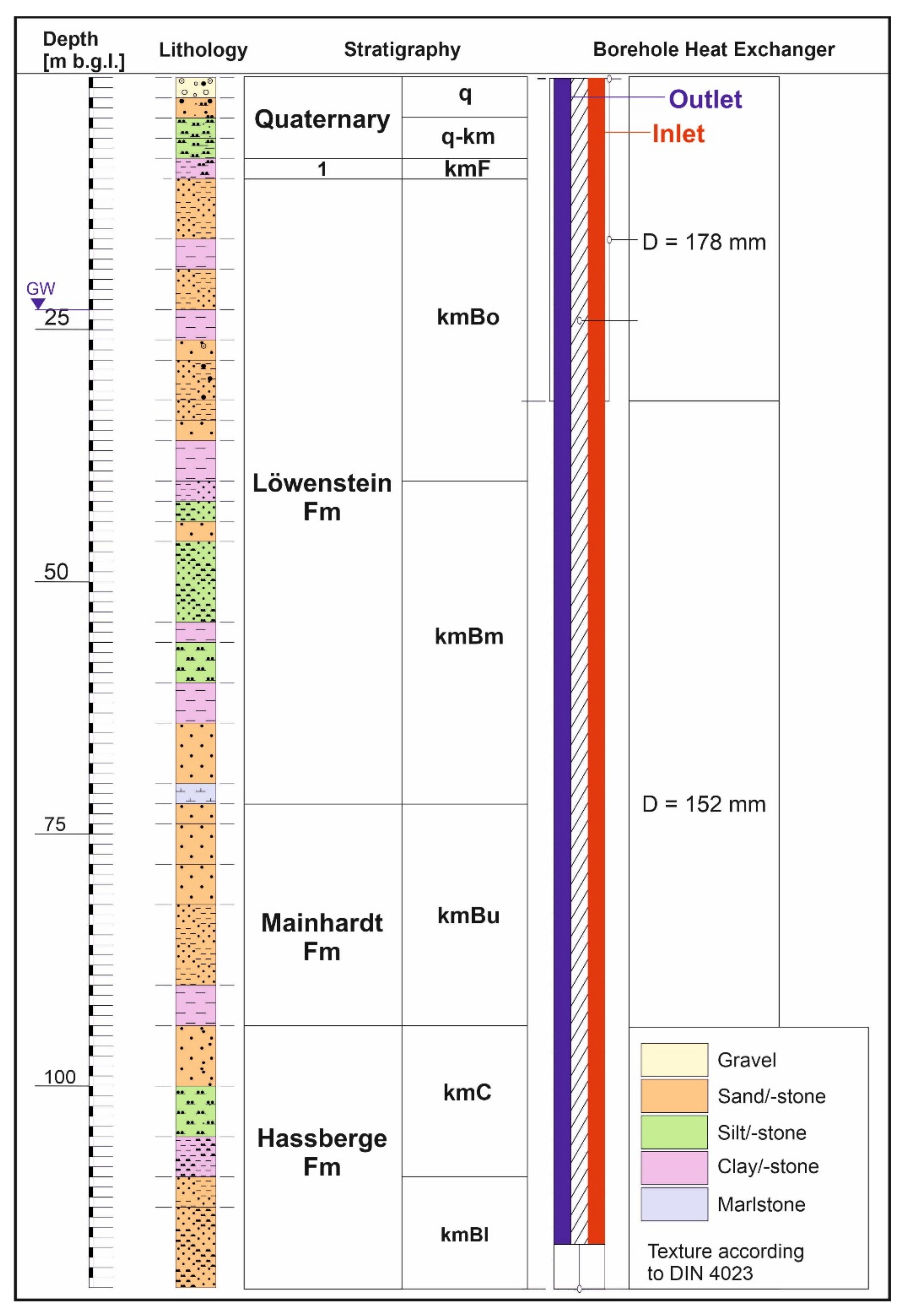
The borehole is located in a lithostratigraphic Quaternary, as well as upper and middle Keuper area [20], which stratigraphically belongs to the Norian and Rhaetian (Triassic) periods. Gravel, sand, and silty Quaternary soils occur down to a depth of 8 m. These are underlain by mudstones, sandstones, and isolated siltstones of Trossingen and Löwenstein formations (upper to middle Keuper) down to a depth of 70 m b. g. l. Below are marlstones, sandstones, and mudstones from Mainhardt formations down to a depth of 94 m b. g. l., as well as sandstones, siltstones, and mudstones comprising Hassberge formations down to the bottom of the BHE at 120 m b. g. l. [20,21]. Figure 1 shows the profile of the drilled borehole, with a focus on lithology and the construction of the probe. Groundwater was detected during the drilling process in summer 2020 at a depth of 23 m b. g. l. In contrast, the hydrogeological map of Bamberg [22] showed groundwater isohypsis at the test site 9 located at 10 m b. g. l. flowing to the southwest.

The BHE and all those that have already been planned are common double-U-tube heat exchangers made of PE 100-RC (polyethylene resistant-to-cracks), with an outer diameter of 32 mm and a wall thickness of 3 mm. The borehole was drilled to 32 m, with a diameter of 178 mm, and to 120 m, with a diameter of 152 mm. The shank spacing is 80 mm. The thermal conductivity of the grout is at λ = 2.40 W/(m∙K). Regular water was used as a heat carrier fluid. All of the specifications of the BHE are listed in

Table 1. Characteristics of the double-U borehole heat exchanger (BHE) and the mobile TRT device; depth in meters below ground level (b. g. l.).

Pilot BHE	Lagarde Campus Bamberg
	Parameters
Borehole length [m]	120
Collector geometry	Double-U-tube
Borehole diameter [mm]	32 m b. g. l.: 178; 120 m b. g. l.: 152
Pipe material	PE 100-RC: Polyethylene resistant-to-cracks
Outer pipe diameter [mm]	32
Pipe thickness [mm]	3
Shank spacing [mm]	80
Pipe thermal conductivity [W/(m∙K)]	0.40
Grouting type	Fischer GeoSolid 240HS
Grouting thermal conductivity [W/(m∙K)]	2.40
Heat carrier fluid	Water
Mobile TRT Rag	Operating Parameters
	Type	Accuracy
Temperature sensors	PT-100	±0.1 °C
Flow meters	Ultrasonic	±0.1%
Data acquisition instrument	Diehl IZAR Center	-
Data logger	D+K Microlog2	±0.1%
	Measured values	Variation
Mean injected heat [W]	5380	±100
Power of heater [kW]	6000
Average operating pressure [MPa]	0.14	±0.01
Mean volume flow rate [m3/h]	1.35	±0.1
Measurement time step [min]	1	-

.

2.2. Mobile TRT Unit

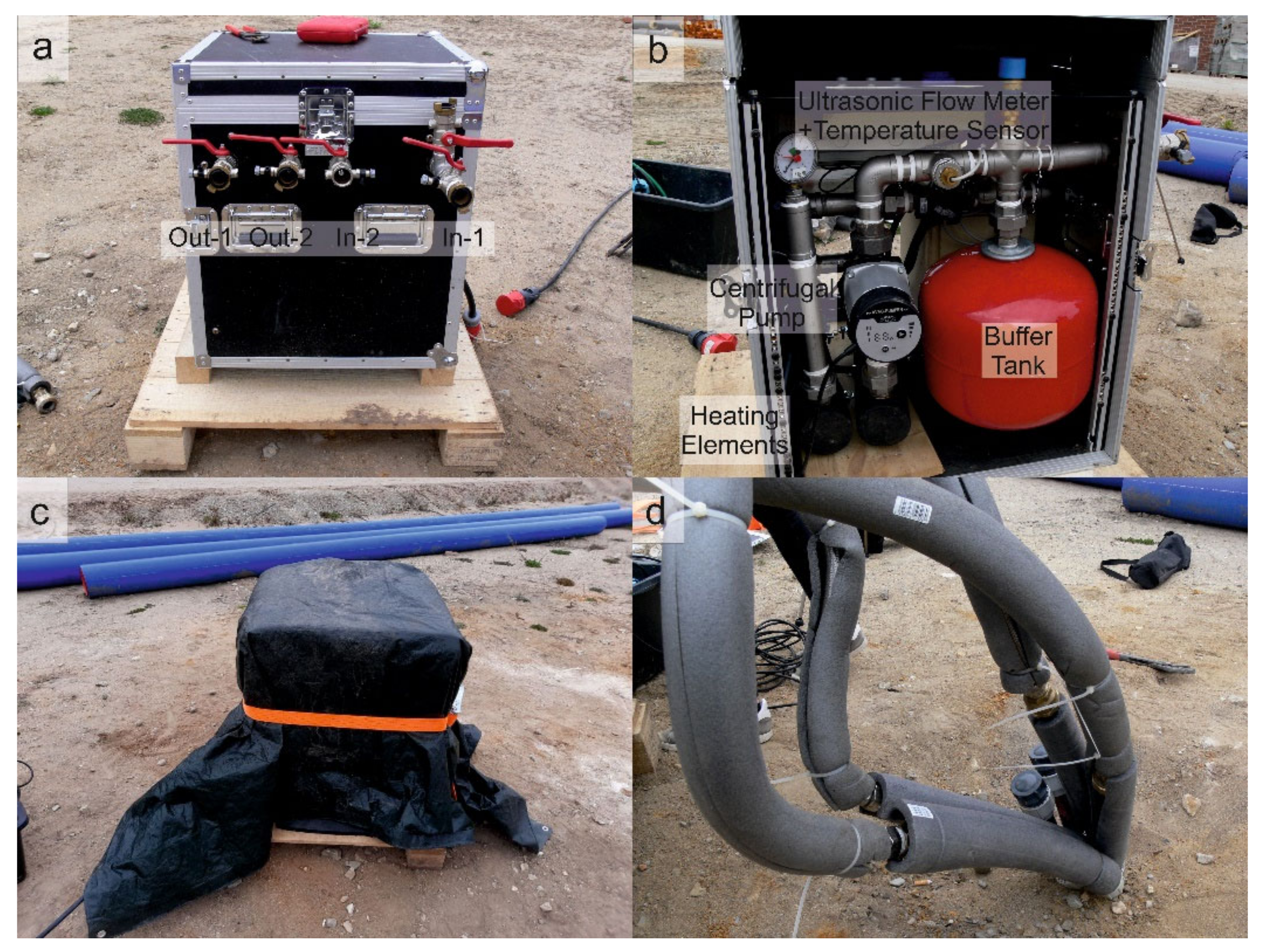
The measuring device that was used is a special customization of a conventional TRT device built by the company Geotechnisches Umweltbüro Lehr. The device has two heating elements with 6 kW and 3 kW of heating power, which can be coupled together or operated separately. The heating power of the 6 kW unit can be continuously adjusted and thus be used for different applications. The device has a main and a secondary circuit that can be shut off via taps (Figure 2a). The built-in centrifugal pump can also provide an adjustable flow at different power levels (see Figure 2b). Calibrated, paired sensors are used to measure the temperature. These are additionally located inside the area in which the flow sensors are housed to keep the measuring errors as low as possible. To determine the subsurface temperatures, a MicroLog pressure–temperature–data logger device was used. It calculates the BHE depth via the pressure of the water column and the pipe properties. This serves as an accurate determination of the (undisturbed) ground temperature, in addition to the determination via the circulation of the heat-carrier fluid [24]. Furthermore, due to the small BHE diameter of 32 mm, temperature measurements are assumed to only be marginally disturbed by thermal convection [25]. The TRT device, which was used by being placed on a transport rack, is insulated by insulation mats made of natural rubber that have a thickness of 19 mm and a maximum thermal conductivity of λ = 0.039 W/(m∙K) at 40 °C (see Figure 2c). The steel connection tubes to the BHE (length: 1 m) are fitted with insulation hoses made of PE that are 13 mm in thickness and that have a maximum thermal conductivity of λ = 0.040 W/(m∙K) at 40 °C (see Figure 2d). Due to the insulation and an additional weather cover, the surface temperature-related influences on the measurements can be kept as low as possible. Table 1 shows the main specifications of the testing rig.

2.3. Evaluation Methods

The evaluation of the gained data was mainly carried out using the programs Geologik TRT 2.0 [26] and MATLAB R2022a. For the one-year measurement series, three different approaches were used to evaluate and determine the thermal parameters: the infinite-line-source, the moving-infinite-line-source theories, the cylinder-source theory, which are explained in the following chapters. For the calculation of the three theories, certain input parameters are required. These can be determined directly by means of the built-in sensor technology of the TRT device or by additional measurements.

2.3.1. Borehole Thermal Resistance

The borehole thermal resistance R_b represents the thermal resistance between the fluid in the BHE’s tubes and the borehole wall. It is a key performance characteristic of closed-loop borehole heat exchangers [27]. Since the discovery and identification of borehole resistance by Morgensen in 1983 [28], many methods and approaches have been published on its determination. In this work, the following formulas are used to determine borehole thermal resistance. R_b is calculated by Equation (2), which is obtained by transformation from Equation (1) for mass flow rate (m) [29,30].

$$m=\frac{Q}{L}\left[\frac{1}{4\pi \lambda }\left(ln\left(\frac{4\alpha }{r_b^2}\right)-\gamma \right)+R_b\right]+T_b$$

(1)

$$R_b=\frac{L}{Q}\left(m-T_b\right)-\frac{1}{4\pi \lambda }\left(ln\left(\frac{4\alpha }{r_b^2}\right)-\gamma \right)$$

(2)

Thermal diffusivity is given by α, borehole radius and borehole wall temperature are expressed by r_b and T_b, and the Euler constant is denoted by γ. The length-related constant heat exchange rate q_l [W/m] can be calculated from the total power input Q [kW], divided by the installation length L [m]. The power input is, in addition to the measured values, determined by the fluid temperature (ϑ) differences between inlet and outlet (also used by Sakata, et al. [31]), with C_p and ρ being the specific heat capacity and the density of the used fluid, in this case water, and the flow rate V:

$$Q=\rho C_{p}V\left({\vartheta }_{in}-{\vartheta }_{out}\right)$$

(3)

when determining R_B, the flow rate at an operating time >12 h is used in order to ensure a stable value [29,32]. The water change is calculated by the total volume Vol [m³] (probe volume + device volume), divided by the flow rate V [m³/s].

2.3.2. Infinite-Line-Source Model (ILS)

Kelvin’s line-source model was already being used in around 1950 to determine the thermal parameters of the first ground-coupled heat pumps [33,34]. The model is the most commonly used evaluation procedure for conventional TRT in practical use. VDI 4640 sheet 5 [30] defines

$$\Delta \vartheta \left(r,t\right)=Q_H\left(\frac{R_B}{2\pi }+\frac{1}{4\pi \lambda }Ei\left(\frac{r^2}{4at}\right)\right)$$

(4)

where the temperature difference Δϑ is a function of radius r and time t. Ei is used for the exponential integral, and a is used as temperature coefficient defined by thermal conductivity divided by volumetric heat capacity.

$$\Delta \vartheta \left(t\right)=Q_{H1}\left(\frac{R_B}{2\pi }+\frac{1}{4\pi \lambda }Ei\left(\frac{r^2}{4at}\right)\right)+{\displaystyle \sum }_{i=2}^n\left(Q_{Hi}-Q_{Hi-1}\right)\left(\frac{R_B}{2\pi }+\frac{1}{4\pi \lambda }Ei\left(\frac{r^2}{4a\left(t-t_{i-1}\right)}\right)\right)$$

(5)

When applying the average temperature difference to the natural logarithm of time, it results in a function with the slope k. This can be determined by simple linear regression and used in the following equation to determine the thermal conductivity, as also stated by VDI 4640 [30]:

$$k=\frac{Q}{H 4 \pi \lambda } \to \mathsf{\lambda }=\frac{Q}{H 4 \pi k}$$

(6)

2.3.3. Infinite-Cylinder-Source Model (ICS)

As shown by [6], evaluation of the cylinder source is a potential model for approaching the thermal parameters of the TRT in the non-steady state and in the quasi-stationary state. Therefore, the gained data were evaluated using the software-implemented cylinder-source model, as shown in Equation (7) [6,26].

$$\Delta \vartheta \left(r,t\right)=\frac{Q_H}{2\pi }\left(R_B+\frac{1}{\lambda }\underset{\sqrt{\frac{r^2}{2at}}}{\overset{\infty }{{\displaystyle \int }}}\frac{e^{-u^2}}{u}{I}_0\left(u^2\right)Erf\left(\frac{L}{2r}\frac{u}{\sqrt{2}}\right)du\right)$$

(7)

The equation above cannot be solved analytically and was approximated numerically by GeoLogik TRT software. Due to this, calculations can be complex and time-consuming, especially due to the repetitive iterations.

2.3.4. Moving-Infinite-Line-Source (MILS) Model

Since the ILS only gives appropriate estimations when the BHE is under very particular hydrogeological conditions, a third model was included. The moving-infinite-line-source (MILS) model takes into account the flow and influence of groundwater. In addition to the ILS model, the MILS model is used in practice, as it considers conductive and advective heat transport [14]. If the groundwater flow around the test site has a Darcy velocity υ_D larger than 10⁻⁷ m s⁻¹, then the infinite-line-source model provides unreliable estimates of thermal conductivity [35]. The general form for the MILS is given in Equations (8) and (9) [14].

$$\Delta T=\frac{q}{4\pi k}{e}^{\frac{r\cos \theta {\upsilon }_T}{2\alpha }}{{\displaystyle \int }}_{r^2/4\alpha t}^{\infty }\frac{1}{\psi }{e}^{-\psi -\frac{1}{\psi }\left(\frac{r{\upsilon }_T}{4\alpha }\right)}d\psi$$

(8)

The ψ is used as an integration variable, and θ defines the angle with the x-axis. The velocity of effective heat transport υ_T is given by division of volumetric heat capacities of the fluid, in this case water, C_w, and the ground C, together with the Darcy velocity:

$${\upsilon }_T=\frac{C_w}{C}{\upsilon }_D$$

(9)

The MILS model involves an integral for which no closed-form expression is known; thus, solving this integral requires a numerical quadrature [14]. A new work by Pasquier and Lamarche [14] further used the Hantush Well function [36], as seen in the integral of Equation (8) and in its reprocessing [37], as well as experimental approaches [38], to develop an analytical expression of the MILS model, as shown in Equation (10).

$$\Delta \overline{T}=\frac{q{I}_0\left(2\sqrt{b}\right)}{4\pi \lambda }\left(Ei\left(\frac{1}{\tau }\right)I_0\left(2\sqrt{b}\right)+e^{-\frac{1}{\tau }}{\displaystyle \sum }_{m=0}^{\infty }{\displaystyle \sum }_{n=m+1}^{\infty }{\left(-\tau \right)}^{m+1}m!\frac{b^n}{n{!}^2}\right)$$

(10)

where I₀ is the modified Bessel function of the first kind and of order 0, and τ and b are parameters used to express the Fourier number (F_o = αt/r²; τ = 4 F_o) and the Péclet number (Pé = rυ_T/α; b = (Pé/4)²) [14]. To calculate the thermal parameters, a MATLAB script was created during a Master’s thesis [39], and this script was also applied in this work.

3. Results

Table 2. Summary of duration and analysis results for thermal response tests using infinite-line-source (ILS), cylinder-source (CS), and moving-infinite-line-source (MILS) models.

Measurement	Duration [h]	λILS [W/(m∙K)]	λICS [W/(m∙K)]	λMILS [W/(m∙K)]	CV [MJ/(m3∙K)]	RB [(m∙K)/W]
March 2021	62.8	2.90	2.93	2.83	0.81	0.121
April 2021	96.7	2.98	3.00	2.93	0.86	0.124
May–June 2021	90.5	2.93	2.97	2.90	0.84	0.130
July 2021	91.8	2.91	2.93	2.92	0.83	0.132
August 2021	88.9	2.99	3.03	2.95	0.70	0.131
September 2021 1	96.1	2.84	2.88	2.90	0.58	0.148
October 2021	95.2	3.05	3.09	2.98	0.64	0.134
November 2021	99.2	3.03	3.06	2.97	0.72	0.130
December 2021	94.6	3.05	3.08	2.99	0.87	0.120
January 2022	95.6	3.05	3.06	2.97	0.9	0.124
February 2022	94.8	3.10	3.13	3.05	0.69	0.126
March 2022	95.5	3.04	3.07	2.97	0.82	0.125

¹ Data from September are not valid due to an interruption in the power supply.

summarizes the test configuration and analysis results of the 12 TRTs. The average measurement period was 5,508 min, with an exception in March 2021 caused by restrictions on the construction site. The calculated thermal conductivities λ range from 2.90 W/(m∙K) in March 2021 up to 3.10 W/(m∙K) in February 2022, according to the line source model, and slightly higher values are achieved for the calculation carried out using the cylinder-source model, ranging from 2.87 to 3.13 W/(m∙K). When using the MILS model, the conductivities are lower compared to the others. In general, the calculations of the three models show no greater deviation from each other than 0.05 W/(m∙K) between ILS and ICS and 0.09 W/(m∙K) between ILS/ICS and MILS. The thermal borehole resistance displays values from 0.12 (m∙K)/W to 0.134 (m∙K)/W. Data from September 2021 are included for completeness, but are not used for further discussion, since a 35-min power outage interrupted heating and fluid circulation. This resulted in lower thermal conductivity and volumetric heat capacity values of λ = 2.84–2.90 W/(m∙K) and C_V = 0.58 MJ/(m³∙K), as well as a higher thermal borehole resistance value, R_B = 0.148 (m∙K)/W.

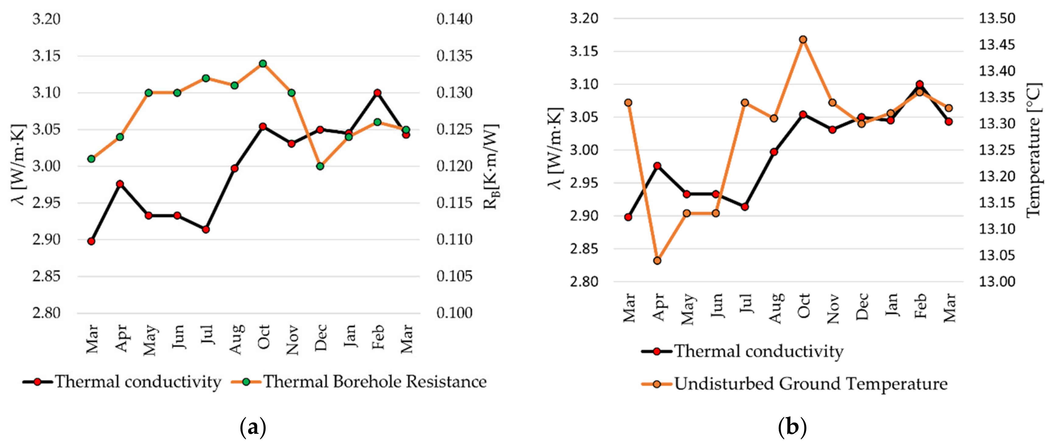
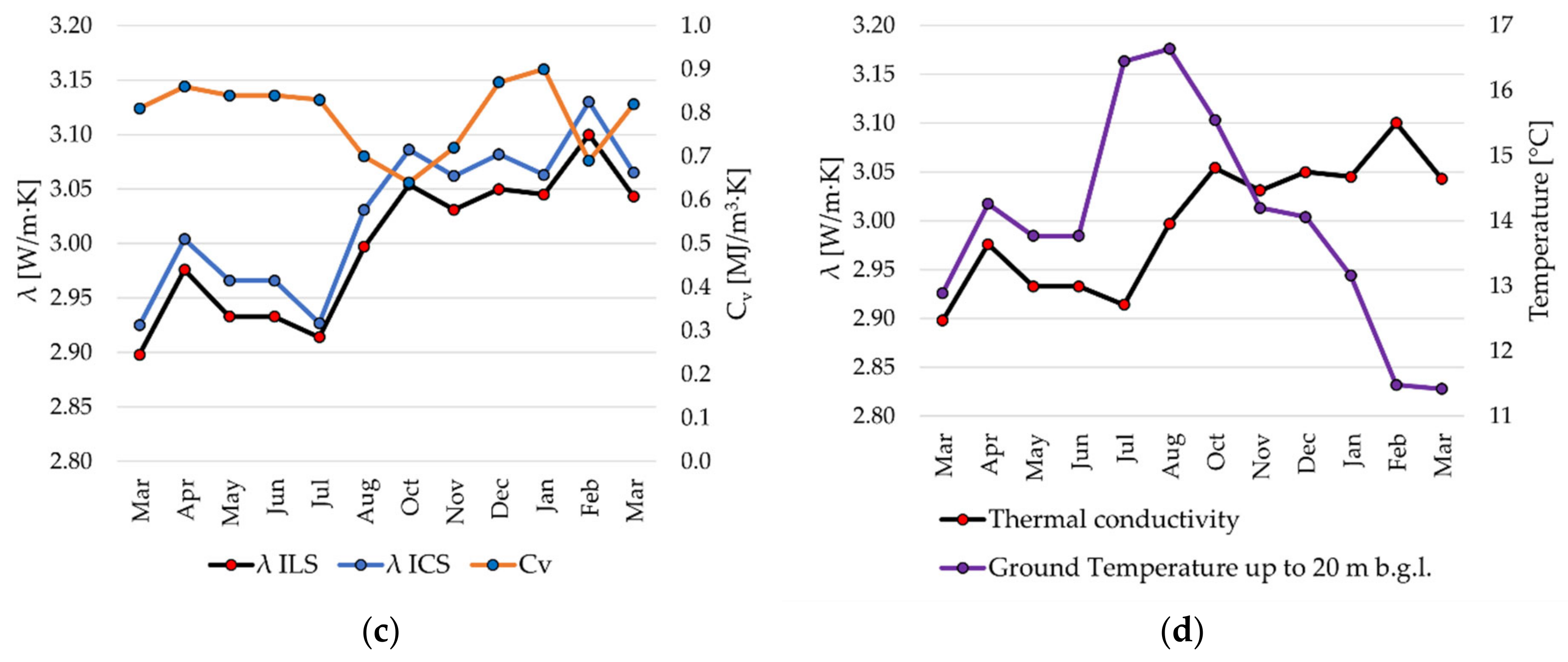
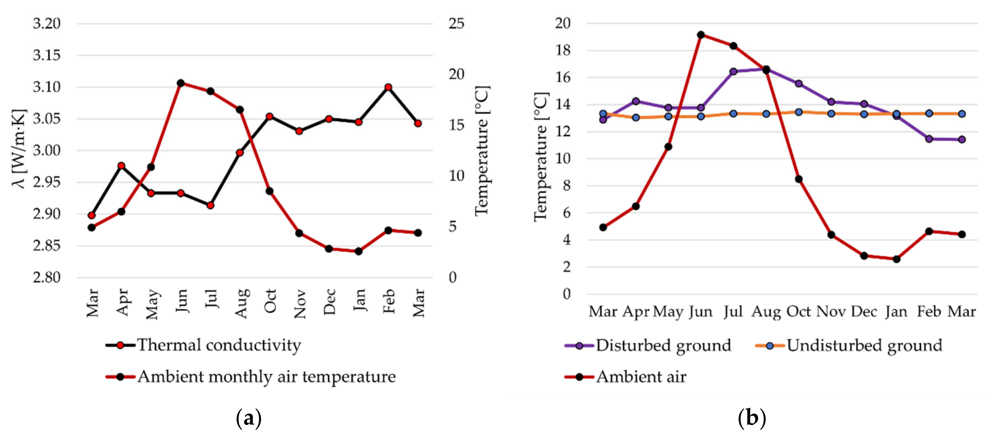
The undisturbed ground temperature at a depth from 20 m to 120 m b. g. l. was measured to be between 13.04 °C (April 2021) and 13.46 °C (October 2021), with a mean of 13.28 °C. The disturbed ground temperature up to 20 m b. g. l. showed high mean values in the summer months of 16.45–16.64 °C (July and August) and low values in the winter months of 11.48–11.42 °C (March and February), with a mean annual temperature of 14.50 °C.

To visualize the results, different thermal conductivity plots were made (see Figure 3a–d). The graphs show the conductivity versus thermal borehole resistance, the temperature of undisturbed and disturbed regions of the BHE, and a comparison of the three evaluation methods: infinite line source, moving infinite line source, and cylindrical source.

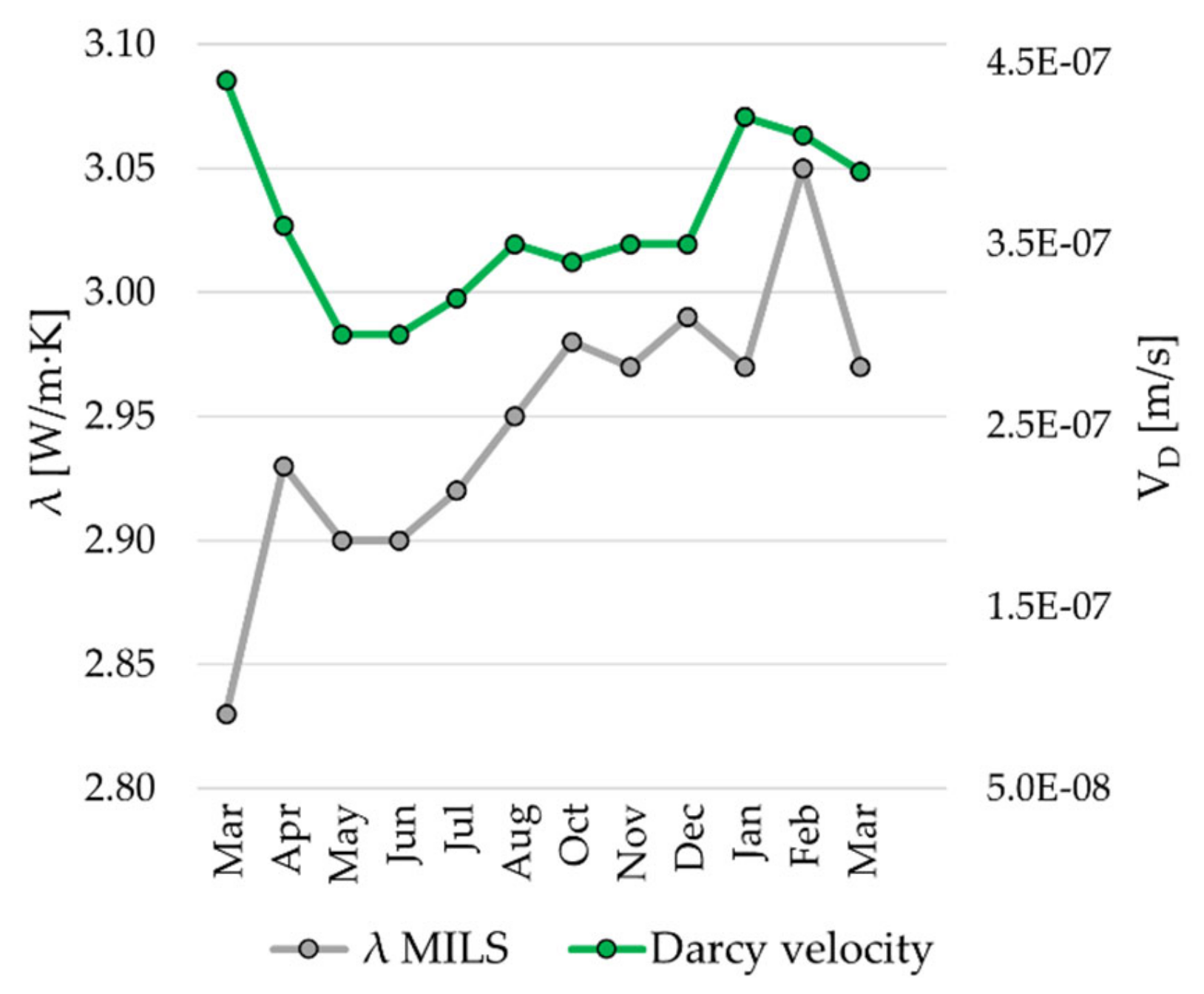
The MILS model calculations resulted in a Darcy velocity for each TRT that was performed. The values range from 3.0 × 10⁻⁷ to 4.4 × 10⁻⁷ m/s. The deviation of each calculated model—ILS, CS, and MILS—is displayed in Figure 4, with 0 W/(m∙K) representing the mean values, as follows: λ_ILS = 2.99 W/(m∙K), λ_ICS = 3.01 W/(m∙K), and λ_MILS = 2.94 W/(m∙K).

4. Discussion

In order to obtain a reasonable result regarding the seasonal influence of the thermal parameters, the following issues are reviewed in the discussion and are matched with our newly determined dataset.

4.1. Influence of on-Site Groundwater Flow

The first important aspect to mention in further discussions is the influence of the groundwater on the BHE. Since no monitoring wells were installed to measure groundwater flow directly, only data calculated using the MILS model can be used. As stated above, Darcy velocities V_D ≥ 10⁻⁷ m/s lead to inaccuracies in the evaluation when ILS is used [35]. Figure 5 shows the correlation of MILS-λ with the calculated V_D. Values are proportional, except in the months of March 2021 and February 2022, but due to the small deviation, a rounding error in the MATLAB script cannot be excluded. By comparing the thermal conductivity values obtained from the ILS, ICS, and MILS models, no deviation > 0.1 W/(m∙K) can be seen. Thus, the low velocities and the small differences in the thermal conductivity indicate no or a very small influence of the groundwater flow to the BHE. However, this has to be investigated regarding the whole heat exchanger field, especially since even small temperature drifts can influence adjacent BHEs.

4.2. Influence of the Device Insulation and Ambient Air Temperature

As mentioned in Section 2, the TRT device is fitted with different forms of insulating materials around the steel hoses and the casing (see Figure 2c,d). Even though VDI 4640-05 [30], as well as discussions by various groups [5,10,40,41], specify the thermal sealing of the device, the effect of ambient air temperature on the device has strong interference when attempting to demonstrate climatic impacts on the ground using an experimental approach. Previous works dealing with in situ TRTs [41,42,43] experienced this connection between fluid temperature in the BHE and ambient air temperature. However, this disturbance by surface temperature decreases with the depth of the borehole and with better insulation [44]. An initial test carried out in August 2020, with the same device on the same BHE, resulted in a thermal conductivity of λ_ILS = 2.70 W/(m∙K), showing a deviation of 0.29 W/(m∙K), although a lower undisturbed ground temperature was measured. This is due to the casing being insufficiently insulated. As can be seen in Figure 6, the thermal conductivity behaves in the opposite way as compared to that which was expected. While the measurements taken in March and April 2021 match the mean outdoor temperature obtained from the weather station in Bamberg [45], the conductivities continue to increase until February 2022. Regarding the thermal borehole resistance, the values of 0.129 ± 0.01 (m∙K)/W are in a normal range compared to other studies [1,10,46] and, therefore, show no external input.

4.3. Climatic Effects on the Underground

A first topic to discuss regarding the site in Bamberg is the urban heat island (UHI) effect [47,48,49]. This phenomenon includes the heating of underground soil and rocks, as well as groundwater [50]. Buildings, especially those with heated basements, or sewer systems, can heat the ground. In Bamberg, this could occur in the historic city center, but the test area is a former military ground that has only begun to be developed into a residential area in the last few years. In principle, there is an area of several hundred meters around the BHE field that was not in use during the TRT period. Still, the heat anomaly can be identified by comparing the measured values with the mean value of the ground temperature obtained via an extensive measuring program carried out by the former Bavarian Water Law Authority, now the Bavarian Environment Agency [51]. The nearest monitoring well, which is located approx. 15 km outside of the urban area of Bamberg, shows a mean groundwater temperature of 10.75 ± 2.15 °C. The mean values of both the disturbed (up to 20 m b. g. l.) and undisturbed temperatures (zone below) are significantly higher, with values of 13.28 ± 0.24 °C and 14.50 ± 3.08 °C, respectively. Considering this, a temperature increase due to the UHI occurs throughout the year.

A factor that has not been mentioned so far is the influence of the geothermal gradient. Other groups [11,52] have demonstrated that the standard TRT does not cover the geothermal gradient and have even showed that, depending on the intensity of impact, the estimation error of the main thermal parameters can exceed 10 % [15,52]. An increase in temperature can be seen in the temperature profile measurements measured from a depth of 80 m b. g. l. through all measurements, with values ranging from 12.95 ± 0.21 °C to 13.26 ± 0.22 °C. We interpret this as a small geothermal gradient that does not influence the comparison of the tests. One factor that is not included in the climatic properties is the moisture of the soil near surface, which varies with the seasons [53]. Water content and soil properties in general, e.g., bulk density, have a commonly known influence on thermal properties [54,55,56]. A good approach could be the long-term monitoring of moisture, temperature, and heat flux using appropriate sensor technology at different depth levels.

By minimizing all of the possible interfering factors mentioned above, including moisture and groundwater flow, insulation, and ambient air, and considering the UHI effect as well as the geothermal gradient as factors that are applicable to all measurements, a cautious step towards seasonal temperature variations can be achieved. The seasonal changes in ground temperature are mainly driven by the absorption of solar energy into the ground, together with decreased heat levels and increased levels between the ground and air [57]. The correlations of interest are shown in Figure 3b,d. While the temperatures in the subsurface down to 20 m b. g. l. decrease, the estimated conductivities rose from summer 2021 to midwinter 2022, implying an opposing trend of thermal conductivity to the upper lithological regime. Together with Figure 6, this relationship can be explained by the offset caused by the thermal storage capacity of the ground. The delay is visible as a sinusoidal wave pattern of ground temperature over time, with increasing lag being observed in temperature change at depth [17]. This is also caused by the thermal inertia on heat transfer in soil. Figure 4 shows the maximum deviations in thermal conductivity for each model and confirms the numerical approaches by Jensen-Page et al. [17] regarding the sizing of the BHE. In contrast to their numerical approaches, we can detect a change in the thermal conductivity. Despite the small changes in λ and R_B, a TRT in winter would lead to an undersized heat exchanger due to better heat transfer conditions and vice versa in summer. If this were applied to a shallower BHE with larger seasonal ambient temperature variations, this effect would be even more significant.

4.4. Comparison of the Performed TRT with Previous Field Tests

The values of the determined thermal conductivities are typical for the surrounding lithological units and Quaternary and Triassic soils [58,59]. The measurements are slightly higher than the referential values of sandstone for the calculation of geothermal systems defined in German VDI 4640, part 1 [60]. We chose various works describing in situ TRT using mostly similar evaluation methods (ILS) to compare the thermal properties under similar conditions. The data from Italy [61] (double U-BHE, 50 m in sandy–silty–clay sediment), Korea [32] (single U-BHE, 150 m in sandy–clay sediment), Turkey [42] (single U-BHE, 30–90 m in marl), and Japan [46] (single-U-BHE, 50 m in sandy–silty–clay sediment) show lower thermal conductivities in a comparable environment. We could not find data outlining the seasonal temperature influences on TRT determined by direct measurements, but we found data showed similar results, as shown by theoretical approaches [17].

5. Conclusions

This study represents an experimental approach to determine the effects of different influences on in situ thermal response testing. The problem and the topic of seasonal influences should be further investigated in the scientific community. The goal of this work was to initiate other researchers to deal with this topic. By conducting a monthly series of measurements over the course of one year on a pilot borehole heat exchanger in Bamberg, Germany, a new dataset could be created, and variations in the estimated and calculated thermal properties could be determined. To reduce commonly known interference effects, three different analytical approaches for the evaluation of TRT have been made, including the infinite-line-source, cylinder-source, and moving-infinite-line-source models. Our measurements resulted in the following:

• A new dataset collected over a period of one year of TRT measurements with fixed operating parameters was created for the temperate climate zone in Central Europe.
• The main thermal parameter λ and R_b obtained using ILS and MILS range from 2.9 to 3.1 W/(m∙K), from 2.83 to 3.05 W/(m∙K), and from 0.120 to 0.134 (m∙K)/W.
• The ICS and ILS show similar values, and the MILS shows a small influence from groundwater flow.
• An influence of the seasonal temperature variations is visible in the determined parameters.
• TRT performed during the winter period displays higher thermal conductivities and lower thermal borehole resistances.

A comparison of the models with each other shows only a minor deviation in the moving-infinite-line-source model compared to the others, which appears to be caused by the marginal impact of groundwater flow. By comparing the outcomes, namely, thermal conductivity, thermal borehole resistance, and ground temperature, a correlation with the seasonal climate is possible. This shows that conductivities are higher in the winter months and lower in summer, leading to a possible under- or overestimation in the design of a borehole heat exchanger field. In addition, an offset of the thermal parameters caused by slow heat transfer in the ground is visible. The operation of TRTs in different seasons can have an influence on planning. Various influences on temperature, e.g., the urban heat anomaly, groundwater flow, and geothermal gradient, must always be considered, but have only occurred to a minor extent in the area investigated.

For further research, a very good method of investigating this problem might be an extensive analysis of enhanced TRT with distributed temperature sensing and longer measurement periods. This would result in a more accurate representation of the temperature differences within the BHE temperature profile. By deploying simultaneous measurements along the whole length, a climatic and seasonal influence can be better detected.

References

- Gehlin, S. Thermal Response Test: Method Development and Evaluation. Master’s Thesis, Luleå tekniska Universitet, Luleå, Sweden, 2002. [Google Scholar]
- Sanner, B.; Reuss, M.; Mands, E.; Müller, J. Thermal response test-experiences in Germany. In Proceedings of the Proceedings Terrastock, Stuttgart, Germany, 28 August–1 September 2000; pp. 177–182. [Google Scholar]
- Eklöf, C.; Gehlin, S. TED—A Mobile Equipment for Thermal Response Test: Testing and Evaluation. Master’s Thesis, Luleå University of Technology, Luleå, Sweden, June 1996. [Google Scholar]
- Austin, W.A., III. Development of an in situ system for measuring ground thermal properties. Master’s Thesis, Oklahoma State University, Stillwater, OK, USA, 1998. [Google Scholar]
- Sanner, B.; Hellström, G.; Spitler, J.D.; Gehlin, S. Thermal Response Test-Current Status and World-Wide Application. In Proceedings of the World Geothermal Congress, Turkey, Antalya, 24–29 April 2005. [Google Scholar]
- Sass, I.; Lehr, C. Improvements on the Thermal Response Test evaluation applying the cylinder source theory. In Proceedings of the Workshop on Geothermal Reservoir Engineering, Stanford, CA, USA, 31 January–2 February 2011. [Google Scholar]
- Zeh, R.; Ohlsen, B.; Philipp, D.; Bertermann, D.; Kotz, T.; Jocić, N.; Stockinger, V. Large-Scale Geothermal Collector Systems for 5th Generation District Heating and Cooling Networks. Sustainability 2021, 13, 6035. [Google Scholar] [CrossRef]
- Sanner, B.; Hellström, G.; Spitler, J.D.; Gehlin, S. More than 15 years of mobile Thermal Response Test—A summary of experiences and prospects. In Proceedings of the European Geothermal Congress, Pisa, Italy, 3–7 June 2013. [Google Scholar]
- Ingersoll, L.R.; Zabel, O.J.; Ingersoll, A.C. Heat Conduction with Engineering, Geological, and Other Applications; University of Wisconsin Press: Madison, WI, USA, 1954. [Google Scholar]
- Raymond, J.; Therrien, R.; Gosselin, L.; Lefebvre, R. A review of thermal response test analysis using pumping test concepts. Ground Water 2011, 49, 932–945. [Google Scholar] [CrossRef] [PubMed]
- Witte, H.J.L.; van Gelder, G.J.; Spitler, J.D. In Situ Measurement of Ground Thermal Conductivity: The Dutch Perspective. ASHRAE Trans. 2002, 108, 263–272. [Google Scholar]
- Hellström, G. Ground Heat Storage: Thermal Analyses of Duct Storage Systems. Ph.D. Thesis, Lund University, Lund, Sweden, 1991. [Google Scholar]
- Badenes, B.; Mateo Pla, M.; Lemus-Zúñiga, L.; Sáiz Mauleón, B.; Urchueguía, J. On the Influence of Operational and Control Parameters in Thermal Response Testing of Borehole Heat Exchangers. Energies 2017, 10, 1328. [Google Scholar] [CrossRef] [Green Version]
- Pasquier, P.; Lamarche, L. Analytic expressions for the moving infinite line source model. Geothermics 2022, 103, 102413. [Google Scholar] [CrossRef]
- Stauffer, F.; Bayer, P.; Blum, P.; Giraldo, N.M.; Kinzelbach, W. Thermal Use of Shallow Groundwater; CRC Press: Boca Raton, FL, USA, 2013. [Google Scholar]
- Carslaw, H.S.; Jaeger, J.C. Conduction of Heat in Solids; Oxford University Press: Oxford, UK, 1947. [Google Scholar]
- Jensen-Page, L.; Narsilio, G.A.; Bidarmaghz, A.; Johnston, I.W. Investigation of the effect of seasonal variation in ground temperature on thermal response tests. Renew. Energy 2018, 125, 609–619. [Google Scholar] [CrossRef]
- Kavanaugh, S.P. Field tests for ground thermal properties—Methods and impact on ground-source heat pump design. In Proceedings of the SHRAE Winter Meeting, Dallas, TX, USA, 20–24 January 2000. [Google Scholar]
- Mikhaylova, O.; Johnston, I.W.; Narsilio, G.A. Uncertainties in the design of ground heat exchangers. Environ. Geotech. 2016, 3, 253–264. [Google Scholar] [CrossRef]
- Lang, M.; Bader, K. Erläuterungen zur Geologischen Karte von Bayern 1: 25,000 Blatt Nr. 6131 Bamberg Süd; Bayerisches Geologisches Landesamt: München, Germany, 1970. [Google Scholar]
- Lang, M. Geologische Karte von Bayern 1:25,000 6131 Bamberg Süd; Bayerisches Geologisches Landesamt: München, Germany, 1970. [Google Scholar]
- Kus, G. Hydrogeologische Karte von Bayern 1:50,000 L 6130 Bamberg Blatt 1: Grundlagen; Bayerisches Landesamt für Umwelt: Augsburg, Germany, 2008. [Google Scholar]
- DIN. DIN 4023-Geotechnical Investigation and Testing—Graphical Presentation of Logs of Boreholes, Trial Pits, Shafts and Adits; Beuth Verlag GmbH: Berlin, Germany, 2004. [Google Scholar]
- Kurevija, T.; Vulin, D.; Krapec, V. Influence of undisturbed ground temperature and geothermal gradient on the sizing of borehole heat exchangers. In Proceedings of the World Renewable Energy Congress, Linkoping, Sweden, 8–13 May 2011; pp. 8–13. [Google Scholar]
- Bertermann, D.; Rammler, M. Suitability of Screened Monitoring Wells for Temperature Measurements Regarding Large-Scale Geothermal Collector Systems. Geosciences 2022, 12, 162. [Google Scholar] [CrossRef]
- Röhrich, T.; Lehr, C. GeoLogik TRT. 2016. Available online: https://www.geologik.com/trt (accessed on 1 March 2021).
- Javed, S.; Spitler, J.D. Calculation of borehole thermal resistance. In Advances in Ground-Source Heat Pump Systems; Elsevier: Amsterdam, The Netherlands, 2016; pp. 63–95. [Google Scholar]
- Morgensen, P. Fluid to duct wall heat transfer in duct system heat storage. In Proceedings of the International Conference on Subsurface Heat Storage in Theory and Practice, Stockholm, Sweden, 6–8 June 1983; pp. 625–657. [Google Scholar]
- Chang, K.S.; Kim, M.J. Thermal performance evaluation of vertical U-loop ground heat exchanger using in-situ thermal response test. Renew. Energy 2016, 87, 585–591. [Google Scholar] [CrossRef]
- VDI. VDI 4640-5 Thermal Use of the Underground—Part 5: Thermal-Response-Test (TRT); VDI—Platz 1: Düsseldorf, Germany, 2020. [Google Scholar]
- Sakata, Y.; Katsura, T.; Serageldin, A.A.; Nagano, K.; Ooe, M. Evaluating Variability of Ground Thermal Conductivity within a Steep Site by History Matching Underground Distributed Temperatures from Thermal Response Tests. Energies 2021, 14, 1872. [Google Scholar] [CrossRef]
- Bae, S.; Nam, Y.; Choi, J.; Lee, K.; Choi, J. Analysis on Thermal Performance of Ground Heat Exchanger According to Design Type Based on Thermal Response Test. Energies 2019, 12, 651. [Google Scholar] [CrossRef]
- Ingersoll, L.R. Theory of the ground pipe heat source for the heat pump. Heat. Pip. Air Cond. 1948, 20, 119–122. [Google Scholar]
- Ingersoll, L.R.; Adler, F.T.; Plass, H.J.; Ingersoll, A.G. Theory of earth heat exchangers for the heat pump. ASHVE Trans 1950, 56, 167–188. [Google Scholar]
- Verdoya, M.; Imitazione, G.; Chiozzi, P.; Orsi, M.; Armadillo, E.; Pasqua, C. Interpretation of thermal response tests in borehole heat exchangers affected by advection. In Proceedings of the World Geothermal Congress 2015, Melbourne, Australia, 19–24 April 2015; p. 7. [Google Scholar]
- Hantush, M.S.; Jacob, C.E. Non-steady radial flow in an infinite leaky aquifer. Eos Trans. Am. Geophys. Union 1955, 36, 95–100. [Google Scholar] [CrossRef]
- Veling, E.; Maas, C. Hantush well function revisited. J. Hydrol. 2010, 393, 381–388. [Google Scholar] [CrossRef] [Green Version]
- Simon, N.; Bour, O.; Lavenant, N.; Porel, G.; Nauleau, B.; Pouladi, B.; Longuevergne, L.; Crave, A. Numerical and experimental validation of the applicability of active-DTS experiments to estimate thermal conductivity and groundwater flux in porous media. Water Resour. Res. 2021, 57, e2020WR028078. [Google Scholar] [CrossRef]
- Grau, M. Thermal-Response-Test (TRT)—Numerische Modellierung des Grundwassereinflusses mittels MILS-Modell (Moving Infinite Line Source). Master’s Thesis, Friedrich-Alexander-Universität Erlangen-Nürnberg, Erlangen, Germany, 2022. [Google Scholar]
- Gehlin, S.; Spitler, J.D. Thermal response test for BTES applications-state of the art 2001. In Proceedings of the 9th International Conference on Thermal Energy Storage, Warsaw, Poland, 1–4 September 2003; pp. 381–387. [Google Scholar]
- Bandos, T.V.; Montero, Á.; Fernández de Córdoba, P.; Urchueguía, J.F. Improving parameter estimates obtained from thermal response tests: Effect of ambient air temperature variations. Geothermics 2011, 40, 136–143. [Google Scholar] [CrossRef] [Green Version]
- Esen, H.; Inalli, M. In-situ thermal response test for ground source heat pump system in Elazığ, Turkey. Energy Build. 2009, 41, 395–401. [Google Scholar] [CrossRef]
- Florides, G.; Kalogirou, S. First in situ determination of the thermal performance of a U-pipe borehole heat exchanger, in Cyprus. Appl. Therm. Eng. 2008, 28, 157–163. [Google Scholar] [CrossRef]
- Gehlin, S.; Nordell, B. Determining Undisturbed Ground Temperature for Thermal Response Test. ASHRAE Trans. 2003, 109, 151–156. [Google Scholar]
- DWD-ClimateDataCenter. Monthly Mean of Station Observations of Air Temperature at 2 m Above Ground in °C for Germany, Version v21.3. Available online: https://cdc.dwd.de/portal/ (accessed on 15 February 2022).
- Choi, W.; Ooka, R. Interpretation of disturbed data in thermal response tests using the infinite line source model and numerical parameter estimation method. Appl. Energy 2015, 148, 476–488. [Google Scholar] [CrossRef]
- Hemmerle, H.; Ferguson, G.; Blum, P.; Bayer, P. The evolution of the geothermal potential of a subsurface urban heat island. Environ. Res. Lett. 2022, 17, 084018. [Google Scholar] [CrossRef]
- Menberg, K.; Bayer, P.; Zosseder, K.; Rumohr, S.; Blum, P. Subsurface urban heat islands in German cities. Sci. Total Environ. 2013, 442, 123–133. [Google Scholar] [CrossRef] [PubMed]
- Zhu, K.; Blum, P.; Ferguson, G.; Balke, K.-D.; Bayer, P. The geothermal potential of urban heat islands. Environ. Res. Lett. 2011, 6, 044002. [Google Scholar] [CrossRef]
- Taniguchi, M.; Uemura, T.; Jago-on, K. Combined Effects of Urbanization and Global Warming on Subsurface Temperature in Four Asian Cities. Vadose Zone J. 2007, 6, 591–596. [Google Scholar] [CrossRef] [Green Version]
- Willy, H. Grundwassertemperatur–Tiefenprofilmessungen der Bayerischen Wasserwirtschaftsverwaltung; Bayerisches Landesamt für Wasserwirtschaft: München, Germany, 2001; Volume 103. [Google Scholar]
- Wagner, V.; Bayer, P.; Kübert, M.; Blum, P. Numerical sensitivity study of thermal response tests. Renew. Energy 2012, 41, 245–253. [Google Scholar] [CrossRef]
- Illston, B.G.; Basara, J.B.; Crawford, K.C. Seasonal to interannual variations of soil moisture measured in Oklahoma. Int. J. Climatol. J. R. Meteorol. Soc. 2004, 24, 1883–1896. [Google Scholar] [CrossRef]
- Go, G.-H.; Lee, S.-R.; Kim, Y.-S.; Park, H.-K.; Yoon, S. A new thermal conductivity estimation model for weathered granite soils in Korea. Geomech. Eng. 2014, 6, 359–376. [Google Scholar] [CrossRef]
- Bertermann, D.; Schwarz, H. Bulk density and water content-dependent electrical resistivity analyses of different soil classes on a laboratory scale. Environ. Earth Sci. 2018, 77, 570. [Google Scholar] [CrossRef]
- Bertermann, D.; Schwarz, H. Laboratory device to analyse the impact of soil properties on electrical and thermal conductivity. Int. Agrophys. 2017, 31, 157–166. [Google Scholar] [CrossRef] [Green Version]
- Wu, J.; Nofziger, D. Incorporating temperature effects on pesticide degradation into a management model. J. Environ. Qual. 1999, 28, 92–100. [Google Scholar] [CrossRef]
- Long, M.; Murray, S.; Pasquali, R. Thermal conductivity of Irish rocks. Ir. J. Earth Sci. 2018, 36, 63–80. [Google Scholar] [CrossRef]
- Galgaro, A.; Dalla Santa, G.; Zarrella, A. First Italian TRT database and significance of the geological setting evaluation in borehole heat exchanger sizing. Geothermics 2021, 94, 102098. [Google Scholar] [CrossRef]
- VDI. VDI 4640-1 Thermal use of the Underground—Part 1: Fundamentals, Approvals, Environmental Aspects; VDI—Platz 1: Düsseldorf, Germany, 2010. [Google Scholar]
- Zarrella, A.; Emmi, G.; Graci, S.; De Carli, M.; Cultrera, M.; Santa, G.; Galgaro, A.; Bertermann, D.; Müller, J.; Pockelé, L.; et al. Thermal Response Testing Results of Different Types of Borehole Heat Exchangers: An Analysis and Comparison of Interpretation Methods. Energies 2017, 10, 801. [Google Scholar] [CrossRef]