
Evaluation of Weather Information for Short-Term Wind Power Forecasting with Various Types of Models
 , , ,
, , ,
Abstract
:1. Introduction
2. Method
2.1. Data Source
2.2. Forecasting Model
2.2.1. ARIMA and ARIMAX
2.2.2. SARIMA and SARIMAX
2.2.3. GARCH
2.2.4. MLR
2.2.5. SVR
2.3. Model Development and Evaluation
2.4. Statistical Analyses
3. Results
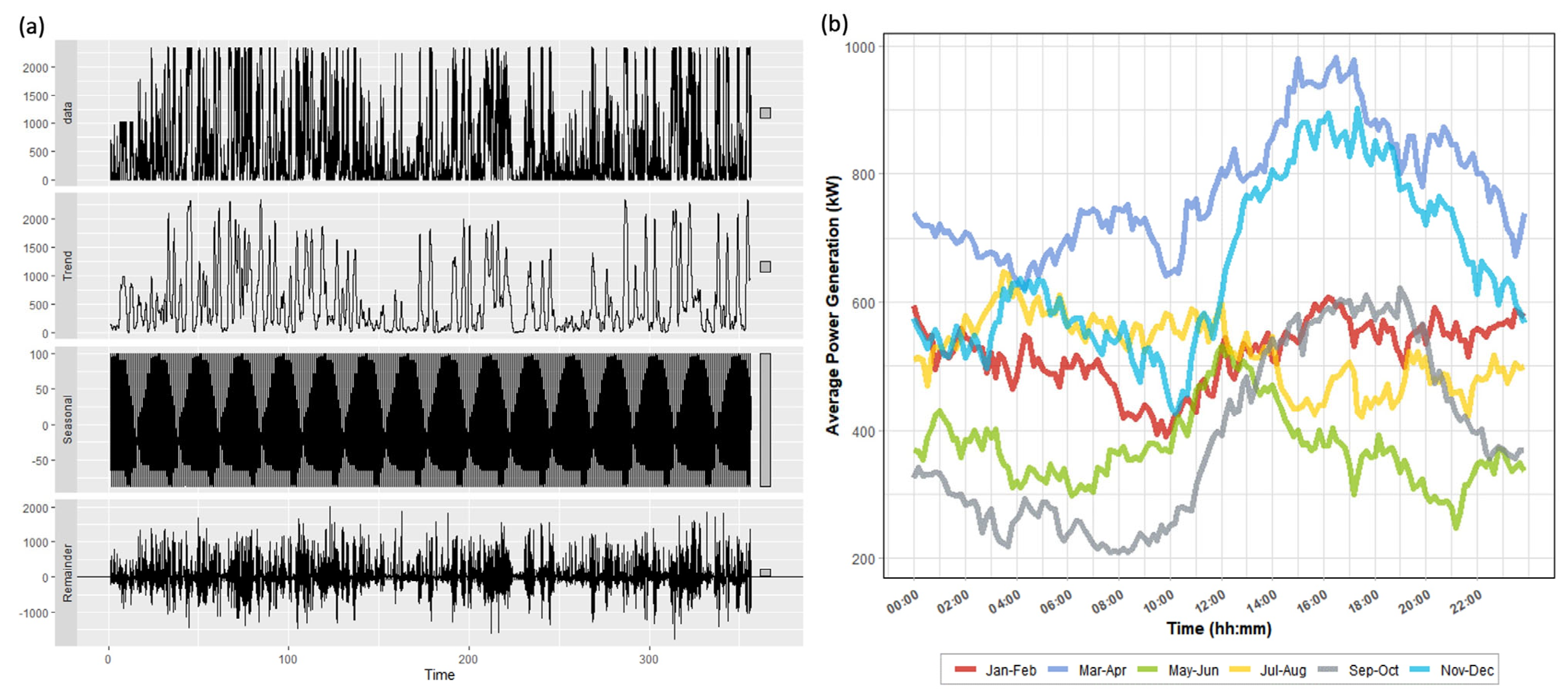
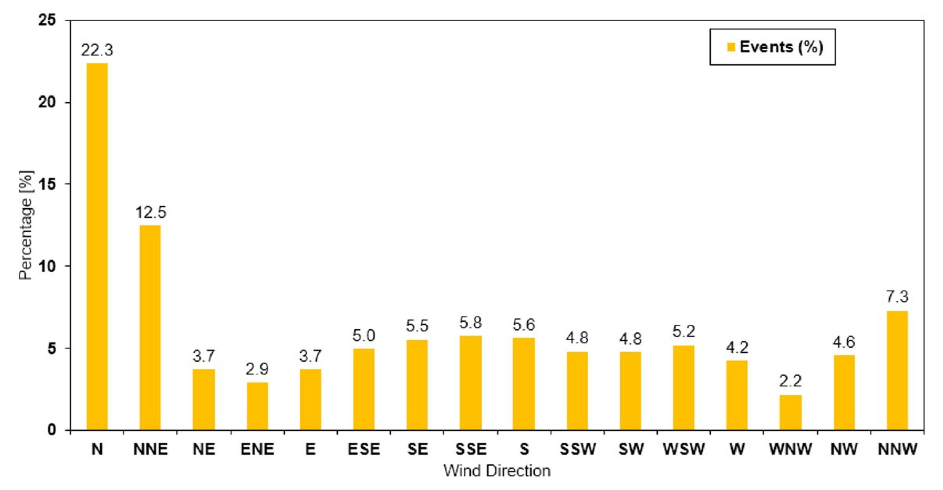
3.1. Data Curation
3.2. Model Optimisation
3.3. Performance Comparison
4. Discussion
5. Conclusions
Author Contributions
Funding
Institutional Review Board Statement
Informed Consent Statement
Data Availability Statement
Conflicts of Interest
Appendix A

| Model | MAE (kW) | NMAE (%) | RMSE (kW) | AIC |
|---|---|---|---|---|
| Single time-series model | ||||
| ARIMA-i | 733.58 | 31.89 | 2904.62 | 150,593.8 |
| SARIMA-i | 687.61 | 29.89 | 2873.40 | 149,480.4 |
| ARIMA-GARCH-i | 1442.76 | 62.70 | 1740.219 | 292,465.1 |
| With weather information | ||||
| MLR-i | 194.97 | 8.48 | 42.439 | 143,138.9 |
| ARIMAX-i | 426.56 | 18.55 | 104.064 | 147,805.1 |
| SARIMAX-i | 400.60 | 17.42 | 91.977 | 147,436.1 |
| SVR-i | 152.25 | 6.62 | 33.900 | Not Available |
References
- Energy Outlook. 2020. Available online: https://www.bp.com/content/dam/bp/business-sites/en/global/corporate/pdfs/energy-economics/energy-outlook/bp-energy-outlook-2020.pdf (accessed on 26 September 2022).
- Cozzi, L.; Gould, T.; Bouckart, S.; Crow, D.; Kim, T.; Mcglade, C.; Olejarnik, P.; Wanner, B.; Wetzel, D. World Energy Outlook 2020; IEA: Paris, France, 2020; pp. 1–461. [Google Scholar]
- Arraño-Vargas, F.; Shen, Z.; Jiang, S.; Fletcher, J.; Konstantinou, G. Challenges and Mitigation Measures in Power Systems with High Share of Renewables—The Australian Experience. Energies 2022, 15, 429. [Google Scholar] [CrossRef]
- International Renewable Energy Agency Abu Dhabi (IRENA). Global Renewables Outlook: Energy Transformation 2050; IRENA: Masdar City, Abu Dhabi, 2020. [Google Scholar]
- Wei, J.; Zhang, Y.; Wang, J.; Wu, L.; Zhao, P.; Jiang, Z. Decentralized Demand Management Based on Alternating Direction Method of Multipliers Algorithm for Industrial Park with CHP Units and Thermal Storage. J. Mod. Power Syst. Clean Energy 2022, 10, 120–130. [Google Scholar] [CrossRef]
- Xiao, L.; Wang, J.; Dong, Y.; Wu, J. Combined forecasting models for wind energy forecasting: A case study in China. Renew. Sustain. Energy Rev. 2015, 44, 271–288. [Google Scholar] [CrossRef]
- Wang, J.; An, Y.; Li, Z.; Lu, H. A novel combined forecasting model based on neural networks, deep learning approaches, and multi-objective optimization for short-term wind speed forecasting. Energy 2022, 251, 123960. [Google Scholar] [CrossRef]
- Frías-Paredes, L.; Mallor, F.; Gastón-Romeo, M.; León, T. Assessing energy forecasting inaccuracy by simultaneously considering temporal and absolute errors. Energy Convers. Manag. 2017, 142, 533–546. [Google Scholar] [CrossRef]
- Jung, J.; Broadwater, R.P. Current status and future advances for wind speed and power forecasting. Renew. Sustain. Energy Rev. 2014, 31, 762–777. [Google Scholar] [CrossRef]
- Hanifi, S.; Liu, X.; Lin, Z.; Lotfian, S. A critical review of wind power forecasting methods—Past, present and future. Energies 2020, 13, 3764. [Google Scholar] [CrossRef]
- Bazionis, I.K.; Georgilakis, P.S. Review of deterministic and probabilistic wind power forecasting: Models, methods, and future research. Electricity 2021, 2, 13–47. [Google Scholar] [CrossRef]
- Rajagopalan, S.; Santoso, S. Wind power forecasting and error analysis using the autoregressive moving average modeling. In Proceedings of the 2009 IEEE Power & Energy Society General Meeting, Calgary, AB, Canada, 26–30 July 2009; pp. 1–6. [Google Scholar]
- Gomes, P.; Castro, R. Wind speed and wind power forecasting using statistical models: Autoregressive moving average (ARMA) and artificial neural networks (ANN). Int. J. Sustain. Energy Dev. 2012, 1. [Google Scholar] [CrossRef]
- Cao, Y.; Liu, Y.; Zhang, D.; Wang, W.; Chen, Z. Wind power ultra-short-term forecasting method combined with pattern-matching and ARMA-model. In Proceedings of the 2013 IEEE Grenoble Conference, Grenoble, France, 16–20 June 2013; pp. 1–4. [Google Scholar]
- Barbosa de Alencar, D.; de Mattos Affonso, C.; Limão de Oliveira, R.C.; Moya Rodriguez, J.L.; Leite, J.C.; Reston Filho, J.C. Different models for forecasting wind power generation: Case study. Energies 2017, 10, 1976. [Google Scholar] [CrossRef]
- Eldali, F.A.; Hansen, T.M.; Suryanarayanan, S.; Chong, E.K. Employing ARIMA models to improve wind power forecasts: A case study in ERCOT. In Proceedings of the 2016 North American Power Symposium (NAPS), Denver, CO, USA, 18–20 September 2016; pp. 1–6. [Google Scholar]
- Haddad, M.; Nicod, J.; Mainassara, Y.B.; Rabehasaina, L.; Al Masry, Z.; Péra, M. Wind and solar forecasting for renewable energy system using sarima-based model. In Proceedings of the International Conference on Time Series and Forecasting, Gran Carnia, Spain, 25–27 September 2019. [Google Scholar]
- Tena García, J.L.; Cadenas Calderón, E.; González Ávalos, G.; Rangel Heras, E.; Mbikayi Tshikala, A. Forecast of daily output energy of wind turbine using sARIMA and nonlinear autoregressive models. Adv. Mech. Eng. 2019, 11, 1687814018813464. [Google Scholar] [CrossRef] [Green Version]
- Chen, H.; Zhang, J.; Tao, Y.; Tan, F. Asymmetric GARCH type models for asymmetric volatility characteristics analysis and wind power forecasting. Prot. Control. Mod. Power Syst. 2019, 4, 29. [Google Scholar] [CrossRef] [Green Version]
- Chen, H.; Li, F.; Wang, Y. Wind power forecasting based on outlier smooth transition autoregressive GARCH model. J. Mod. Power Syst. Clean Energy 2018, 6, 532–539. [Google Scholar] [CrossRef] [Green Version]
- Amral, N.; Ozveren, C.; King, D. Short term load forecasting using multiple linear regression. In Proceedings of the 2007 42nd International Universities Power Engineering Conference, Brighton, UK, 4–6 September 2007; pp. 1192–1198. [Google Scholar]
- Ryu, J.; Cha, J.; Lee, B. Evaluation of Weather Information in Forecasting Daily Peak Load of Electricity Demand. J. Korean Inst. Illum. Electr. Install. Eng 2018, 32, 73–81. [Google Scholar]
- Chen, Q.; Folly, K.A. Short-Term Wind Power Forecasting Using Mixed Input Feature-Based Cascade-connected Artificial Neural Networks. Front. Energy Res. 2021, 9, 634639. [Google Scholar] [CrossRef]
- Wu, W.; Chen, K.; Qiao, Y.; Lu, Z. Probabilistic short-term wind power forecasting based on deep neural networks. In Proceedings of the 2016 International Conference on Probabilistic Methods Applied to Power Systems (PMAPS), Beijing, China, 16–20 October 2016; pp. 1–8. [Google Scholar]
- Mujeeb, S.; Javaid, N.; Gul, H.; Daood, N.; Shabbir, S.; Arif, A. Wind power forecasting based on efficient deep convolution neural networks. In Proceedings of the International Conference on P2P, Parallel, Grid, Cloud and Internet Computing, Antwerp, Belgium, 7–9 November 2019; pp. 47–56. [Google Scholar]
- Zhang, H.; Chen, L.; Qu, Y.; Zhao, G.; Guo, Z. Support vector regression based on grid-search method for short-term wind power forecasting. J. Appl. Math. 2014, 2014, 835791. [Google Scholar] [CrossRef] [Green Version]
- Park, T.-H.; Jang, D.-S.; Bae, G.-M.; Kim, K.-M.; Ahn, J.-H. Selection of Input variables and comparison of Artificial Neural Networks and one-dimensional Convolutional Neural Networks for Prediction of Wind Power Generation in Yeongheung Wind Power Plant. J. Korean Soc. Environ. Eng. 2021, 43, 219–229. [Google Scholar] [CrossRef]
- Bigdeli, N.; Afshar, K.; Gazafroudi, A.S.; Ramandi, M.Y. A comparative study of optimal hybrid methods for wind power prediction in wind farm of Alberta, Canada. Renew. Sustain. Energy Rev. 2013, 27, 20–29. [Google Scholar] [CrossRef]
- Wang, J.; Zhou, Q.; Zhang, X. Wind power forecasting based on time series ARMA model. IOP Conf. Ser. Earth Environ. Sci. 2018, 199, 022015. [Google Scholar] [CrossRef]
- Duan, J.; Wang, P.; Ma, W.; Fang, S.; Hou, Z. A novel hybrid model based on nonlinear weighted combination for short-term wind power forecasting. Int. J. Electr. Power Energy Syst. 2022, 134, 107452. [Google Scholar] [CrossRef]
- Qin, J.; Yang, J.; Chen, Y.; Ye, Q.; Li, H. Two-stage short-term wind power forecasting algorithm using different feature-learning models. Fundam. Res. 2021, 1, 472–481. [Google Scholar] [CrossRef]
- Liu, R.; Peng, M.; Xiao, X. Ultra-short-term wind power prediction based on multivariate phase space reconstruction and multivariate linear regression. Energies 2018, 11, 2763. [Google Scholar] [CrossRef] [Green Version]
- Qin, G.; Yan, Q.; Zhu, J.; Xu, C.; Kammen, D.M. Day-ahead wind power forecasting based on wind load data using hybrid optimization algorithm. Sustainability 2021, 13, 1164. [Google Scholar] [CrossRef]
- Yu, L.; Ma, Y.; Ma, Y.; Zhang, G. A complexity-trait-driven rolling decomposition-reconstruction-ensemble model for short-term wind power forecasting. Sustain. Energy Technol. Assess. 2022, 49, 101794. [Google Scholar] [CrossRef]
- Korea East-West Power Co., Ltd. Younggwang Baeksu Wind Power Complex Unit 1, 10-Minute Average Power Generation. 2022. Available online: https://www.data.go.kr/data/15091978/fileData.do (accessed on 13 October 2021).
- Burton, T.; Jenkins, N.; Sharpe, D.; Bossanyi, E. Wind Energy Handbook; John Wiley & Sons: Hoboken, NJ, USA, 2011. [Google Scholar]
- Thönnißen, F.; Marnett, M.; Roidl, B.; Schröder, W. A numerical analysis to evaluate Betz’s Law for vertical axis wind turbines. J. Phys. Conf. Ser. 2016, 753, 022056. [Google Scholar] [CrossRef]
- Tang, S.; Yuan, S.; Zhu, Y. Data preprocessing techniques in convolutional neural network based on fault diagnosis towards rotating machinery. IEEE Access 2020, 8, 149487–149496. [Google Scholar] [CrossRef]
- Hyndman, R.J.; Athanasopoulos, G. Forecasting: Principles and Practice; OTexts: Melbourne, Australia, 2018. [Google Scholar]
- Huang, C.-J.; Kuo, P.-H. A short-term wind speed forecasting model by using artificial neural networks with stochastic optimization for renewable energy systems. Energies 2018, 11, 2777. [Google Scholar] [CrossRef] [Green Version]
- Al-Dahidi, S.; Ayadi, O.; Adeeb, J.; Alrbai, M.; Qawasmeh, B.R. Extreme learning machines for solar photovoltaic power predictions. Energies 2018, 11, 2725. [Google Scholar] [CrossRef] [Green Version]
- Khazaei, S.; Ehsan, M.; Soleymani, S.; Mohammadnezhad-Shourkaei, H. A high-accuracy hybrid method for short-term wind power forecasting. Energy 2022, 238, 122020. [Google Scholar] [CrossRef]
- McGrath, M. Python in Easy Steps: Covers Python 3.7. In Easy Steps; In Easy Steps Limited: Southham, UK, 2018. [Google Scholar]
- Quang-Hung, N.; Doan, H.; Thoai, N. Performance evaluation of distributed training in Tensorflow 2. In Proceedings of the 2020 International Conference on Advanced Computing and Applications (ACOMP), Quy Nhon, Vietnam, 25–27 November 2020; pp. 155–159. [Google Scholar]
- Ketkar, N. Introduction to Keras. In Deep Learning with Python; Springer: Berlin/Heidelberg, Germany, 2017; pp. 97–111. [Google Scholar]
- Hyndman, R.J.; Athanasopoulos, G.; Gally, S.; gridExtra, M.; Hyndman, R.; Hyndman, M.R. Package ‘fpp2’. 2020. Available online: https://cran.r-project.org/web/packages/fpp2/index.html (accessed on 9 September 2022).
- Ghalanos, A.; Ghalanos, M.A.; Rcpp, L. Package ‘rugarch’; R Team Cooperation: Vienna, Austria, 2018. Available online: https://cran.r-project.org/web/packages/rugarch/index.html (accessed on 26 October 2022).
- Diebold, F.X.; Mariano, R.S. Comparing predictive accuracy. J. Bus. Econ. Stat. 2002, 20, 134–144. [Google Scholar] [CrossRef]
- Rahman, M.N.; Esmailpour, A.; Zhao, J. Machine learning with big data an efficient electricity generation forecasting system. Big Data Res. 2016, 5, 9–15. [Google Scholar] [CrossRef]


| Variables | Unit | Min.–Max. | Mean ± SD |
|---|---|---|---|
| Wind power | kW | 0.0–2357.9 | 536.8 729.6 |
| Wind speed | m/s | 0.0–36.9 | 7.2 4.6 |
| Wind direction | ° | 0.0–360.0 | 146.9 120.9 |
| Temperature | °C | −9.9–34.5 | 13.3 9.3 |
| Pressure | hPa | 981.7–1032.7 | 1012.5 8.7 |
| Humidity | % | 16.9–99.9 | 75.7 17.6 |
| Model | Parameter | Candidate Range | Final Model |
|---|---|---|---|
| Single time-series model | |||
| ARIMA | p, d, q | 0–10 | ARIMA(3,1,2) |
| SARIMA | p, d, q, P, D, Q | 0–10 for p, d, q 0–12 for P, D, Q | SARIMA(4,1,2)(1,0,2) (144) |
| ARIMA-GARCH | p, d, q, P, Q | 0–10 for p, d, q 0–5 for P, Q | ARIMA(3, 1, 2)-GARCH(1, 1) |
| With weather information | |||
| MLR* | - | - | PG ~ PG(lag 1), WS, WD, AT, HM, TC, SS, AT × SS, HM × TC |
| ARIMAX | p, d, q | 0–10 | ARIMAX(1, 1, 1) |
| SARIMAX | p, d, q, P, D, Q | 0–10 for p, d, q 0–12 for P, D, Q | SARIMA(3, 0, 1)(0,0,1) (144) |
| SVR | Kernel | linear, polynomial, radial bias | radial bias |
| Cost | 1–10 | 2 | |
| Epsilon | 0.1 to 0.9 by 0.05 | 0.15 | |
| Model | MAE (kW) | NMAE (%) | RMSE (kW) | AIC |
|---|---|---|---|---|
| Single time-series model | ||||
| ARIMA | 684.24 | 29.75 | 2847.11 | 150,593.8 |
| SARIMA | 521.46 | 22.67 | 2704.04 | 149,480.4 |
| ARIMA-GARCH | 1447.70 | 62.94 | 17,429.79 | 292,465.1 |
| With weather information | ||||
| MLR | 150.54 | 6.55 | 33.62 | 143,138.9 |
| ARIMAX | 350.28 | 15.23 | 93.13 | 147,805.1 |
| SARIMAX | 300.40 | 13.06 | 84.71 | 147,436.1 |
| SVR | 145.08 | 6.31 | 30.72 | - |
Publisher’s Note: MDPI stays neutral with regard to jurisdictional claims in published maps and institutional affiliations. |
© 2022 by the authors. Licensee MDPI, Basel, Switzerland. This article is an open access article distributed under the terms and conditions of the Creative Commons Attribution (CC BY) license (https://creativecommons.org/licenses/by/4.0/).
Share and Cite
Ryu, J.-Y.; Lee, B.; Park, S.; Hwang, S.; Park, H.; Lee, C.; Kwon, D. Evaluation of Weather Information for Short-Term Wind Power Forecasting with Various Types of Models. Energies 2022, 15, 9403. https://doi.org/10.3390/en15249403
Ryu J-Y, Lee B, Park S, Hwang S, Park H, Lee C, Kwon D. Evaluation of Weather Information for Short-Term Wind Power Forecasting with Various Types of Models. Energies. 2022; 15(24):9403. https://doi.org/10.3390/en15249403
Chicago/Turabian StyleRyu, Ju-Yeol, Bora Lee, Sungho Park, Seonghyeon Hwang, Hyemin Park, Changhyeong Lee, and Dohyeon Kwon. 2022. "Evaluation of Weather Information for Short-Term Wind Power Forecasting with Various Types of Models" Energies 15, no. 24: 9403. https://doi.org/10.3390/en15249403