Fundamental Understanding of Heat and Mass Transfer Processes for Physics-Informed Machine Learning-Based Drying Modelling

Abstract

Drying is a complex process of simultaneous heat, mass, and momentum transport phenomena with continuous phase changes. Numerical modelling is one of the most effective tools to mechanistically express the different physics of drying processes for accurately predicting the drying kinetics and understanding the morphological changes during drying. However, the mathematical modelling of drying processes is complex and computationally very expensive due to multiphysics and the multiscale nature of heat and mass transfer during drying. Physics-informed machine learning (PIML)-based modelling has the potential to overcome these drawbacks and could be an exciting new addition to drying research for describing drying processes by embedding fundamental transport laws and constraints in machine learning models. To develop such a novel PIML-based model for drying applications, it is necessary to have a fundamental understanding of heat, mass, and momentum transfer processes and their mathematical formulation of drying processes, in addition to data-driven modelling knowledge. Based on a comprehensive literature review, this paper presents two types of information: fundamental physics-based information about drying processes and data-driven modelling strategies to develop PIML-based models for drying applications. The current status of physics-based models and PIML-based models and their limitations are discussed. A sample PIML-based modelling framework for drying application is presented. Finally, the challenges of addressing simultaneous heat, mass, and momentum transport phenomena in PIML modelling for optimizing the drying process are presented at the end of this paper. It is expected that the information in this manuscript will be beneficial for further advancing the field.

1. Introduction

Drying is a dominant industrial process that is intensely used for processing or preserving bulk wet materials to inhibit the growth of bacteria, yeasts, and mould through the removal of water. For example, the drying process is widely used in diverse industrial sectors, including the agricultural, wood, seafood, pharmaceutical, paper, ceramic, and biomass processing industries. The current drying market, air drying, in particular, is worth USD 108.15 billion and is expected to be USD 166.92 billion by 2027 [1]. Despite this incredible potential, today’s drying industries have been experiencing difficulties with the existing conventional drying systems, which are energy-intensive, and slow processes. Depending on drying conditions, the drying process can account for up to 15% of all industrial energy usage. Moreover, the deterioration in the quality of the dried products is one of the major problems of today’s drying systems. These problems cannot be solved unless drying systems are designed based on a fundamental understanding of the actual drying process and characteristics of the products at different length scales. The drying process involves complex simultaneous heat, mass, and momentum transport processes [2]. Numerical modelling is a unique tool to accurately describe these complex drying processes [3], and, therefore, significant research has been conducted to develop numerical modelling for drying processes.

Based on the level of accuracy and approaches, the existing drying models can be categorised as first-, second-, third-, fourth-, and fifth-generation models. The first-generation models are purely empirical and depend on the particular products and the drying conditions [4,5]. The specific product and process dependency of the first-generation models restrict their applications to other products or processes. To overcome these problems of the first-generation models, a slightly improved model, called the second-generation model, has been introduced [6]. In this modelling strategy, a physics-based approach is integrated with the empirical modelling approaches. Although these models help to provide a better understanding of drying kinetics, a realistic understanding of drying processes (for example, instantaneous moisture and temperature distribution) cannot be predicted using the second-generation models. This being the case, the next generation of drying models can be referred to as the third generation. They are developed based on fundamental physics-based approaches, such as conservation of mass and energy, Newton’s laws of motion, and Navier–Stokes equations for fluid flow. The third-generation models are sometimes developed based on single-phase (liquid water transport) phenomena [7,8,9,10,11,12,13]. Porous materials, such as food and wood, contain multiple species, including liquid water, gas (vapour and air), and solid content. In drying modelling, consideration of these multiple species is intensely important for an accurate prediction of drying kinetics; therefore, multiphase models are developed [2,14,15,16]. These third-generation models are entirely based on the macro- or tissue scale. However, porous materials, particularly food materials, are multiscale in nature, containing different irregular cellular structures. As the mass transfer processes initiate at the cell level during drying, consideration of the cellular water transport processes is crucial for accurate prediction of drying kinetics and optimising drying processes. To account for both cellular (microscale) and macro- (tissue)-scale water transport processes, multiscale modelling strategies have been introduced. This most advanced level of modelling can be referred to as the fourth generation of drying models. It is important to know the fundamental physics behind the transport phenomena at different length scales to mathematically describe the simultaneous heat and mass transfer processes. Although the aforementioned physics-based models can provide better insights, including the instantaneous and spatial distribution of moisture and temperature, the development of purely physics-based models is intensely challenging and computationally very expensive.

In order to reduce the computational complexity, data-driven modelling, such as machine learning (ML)-based modelling, can be implemented for food drying applications. ML-based approaches can effectively model the nonlinear complex heat and mass transfer processes during drying and are able to predict drying kinetics without much computational effort, such as traditional modelling techniques. However, ML-based models struggle to generate accurate predictions when the dataset is ill-posed, noisy, and insufficient [17,18]. In such cases, the incorporation of physics into observational data through PIML provides promising benefits to most science and engineering applications [18,19,20]. This category of the model can be referred to as the fifth-generation drying model. Although numerous studies have been conducted to develop fundamental physics-based modelling, as well as machine-learning-based models, no PIML-based drying model has been developed taking advantage of both the ML- and physics-based base modelling approaches. To address this major research gap, significant scientific research is required. This paper aims to present the fundamental understanding of the physics that is used for food drying modelling and the potential PIML-based modelling strategies. This paper is sequentially organised by first presenting an understanding of different categories of existing drying models and the necessity of PIML-based modelling in Section 1. Then, the basic drying processes (drying mechanism) are presented in Section 2. The physics that drives the drying processes are discussed in Section 3. Section 4 presents the status of the existing mathematical modelling, including PIML, and its limitations. A sample PIML-based modelling framework is presented in Section 5. Spatial distributions of airflow significantly affect drying kinetics, and, therefore, conjugation of airflow (integration of spatial airflow distribution with the drying model) is important in food drying modelling. An understanding of the airflow conjugate modelling is presented in Section 6. Finally, the current challenges of drying modelling, including PIML-based models, are discussed in Section 7.

2. Drying Mechanism

During convective hot air drying, hot air is supplied across the moist products. The heat transfer occurs from the surface of the products to the centre through conduction, convection, and phase change. Due to the continuous supply of heat energy, mass transfer occurs through evaporation from the surface of the products to the environment. Moreover, the internal mass transfer occurs through diffusion capillary flow and the viscous flow inside the products due to the concentration gradients [21]. A conceptual understanding of the drying process is presented in Figure 1.

The drying processes can be defined by their drying kinetics, such as drying rate, which is the function of moisture content, as shown in Figure 2. Theoretically, the drying rate curve can be divided into three regions. At the beginning of drying, the product is full of moisture content. It could be at Point A or A’, depending on whether the product remains at a cold or hot temperature. Once the drying processes have progressed, a constant drying rate curve can be observed at the early stage of drying (Points “B-C” in Figure 2). During the constant rate period, free moisture evaporates from the surface to the surroundings, and the drying rate remains almost steady. However, this constant rate period sometimes cannot be found in practical applications due to non-uniform heating or uneven product distribution. During the constant rate period, moisture also migrates from the core to the surface through diffusion. This diffusion process is mainly due to the concentration gradient that is developed by the evaporation process of surface moisture. Through this process of drying, the moisture content of the products decreases and reaches its ‘critical moisture content’ point (Point C in Figure 2). This is the time when inequality between evaporation from the surface and water diffusion from the inside to the surface becomes apparent. When the moisture content reaches its critical moisture content point, the drying rate starts to fall, and it gradually decreases. This is mainly due to the lower availability of free water but the greater availability of bound water inside the products. As the bound moisture is tightly held inside the cellular compartment of the products [22], it takes longer to migrate through periodic cell rupture and capillary diffusion processes and becomes free water for transport. Consequently, the drying rate gradually falls, as shown in Figure 2 (“C-D”). During this first falling period, the surface of the product becomes almost dried, as there is insufficient (free) moisture. At this stage, heat energy is continuously supplied to the products to take out the bound moisture, which results in the product surface becoming very hard and forming crusts. This crust formation creates an extra obstacle for the evaporation process from the surface of the products to the environment, and, hence, the drying rate further decreases. This further reduction of the drying rate can be referred to as the second falling rate period, as shown in Figure 2 (“D-E”). It should be mentioned here that the constant rate period is sometimes controlled by external parameters, such as air humidity, air speed, and air temperature. However, the fall rate period is totally dependent on the products’ characteristics and their internal microstructural features.

3. Physics of Convective Drying Process

Drying is a complex simultaneous heat, mass, and momentum transport process, and it is critical to understand the underlying physics in order to describe the drying processes and develop a PIML-based framework. Therefore, the underlying physics behind the drying processes are discussed in this section.

3.1. Mass Transport

Mass transport is simply a process of transporting chemical species from one location to another. During drying, moisture migrates from various cellular locations in the products to the surface of the products due to the concentration gradients, and then the surface moisture is migrated to the environment (drying air) through evaporation [23]. Here, the first process can be defined as an internal mass transport process where moisture moves from one place to another inside the products, and the second can be defined as an external mass transport process where the moisture is transported from the product surface to the drying air inside the dryer, as shown in Figure 1. Porous materials, such as food materials, contain multiphase (solid, liquid, and gas) species inside the products [2,24]. The transport characteristics of liquid water and gas species are different, and, therefore, a different subset of physics is required to mathematically express their transport phenomena. Diffusion, convection, and evaporation are the main driving mechanism of internal and external mass transport. These internal and external mass transport processes can be described and mathematically expressed by different subsets of known physics, which are discussed below.

3.1.1. Diffusion

Diffusion is a molecular mass transfer process where molecules are randomly moved from a higher-concentration area to a lower-concentration region, in which no molecules have a preferred direction. Two different diffusion processes, namely, capillary diffusion and binary diffusion, are used to define the movement of liquid water and gas species, respectively.

Capillary diffusion: Capillary diffusion is a mass transfer process mainly due to the capillary action of the liquid. The capillary action is created by the capillary forces. Capillary forces are the molecular attraction between the liquid molecules and the solid surfaces. Moreover, the interfacial pressure difference inside the porous matrix is responsible for raising the capillary actions [25]. For addressing the liquid species transport in a multiphase domain, the capillary diffusion phenomenon is widely used. For modelling the capillary action into small pores in a multiphase porous domain, the Lucas–Washburn equation is well recognised [26]. In this equation, viscous drag and gravity are considered the balancing parameters of the pressure inside a cylindrical capillary [27,28], which can be expressed by the following expression:

$$h_c=\frac{2\gamma \cos \left(\theta \right)}{r\rho g}$$

(1)

where h_c is the capillary height (m), $\gamma$ is referred to as the surface tension (N/m), $\theta$ is the contact angle (^°), r is the capillary radius (m), $\rho$ is the density of water (kg/m³), and g is the gravitational acceleration (m/s²).

Moreover, the capillary flow in porous media can be expressed by Darcy’s law [14]:

$$u=-\frac{k_l}{\mu } \frac{\partial P}{\partial x}$$

(2)

where P is the fluid pressure (Pa), u is the Darcy velocity (m/s), $k_l$ is the porous material’s permeability (m²), and $\mu$ is the dynamic viscosity (Pa·s).

Sometimes, the capillary action can be expressed as a result of negative pressure on the liquid [14]; therefore, the mass transfer (mass flux) of liquid can be expressed by the following equation:

$$n_l^{pr., capillary}=-{\rho }_l \frac{k_l}{{\mu }_l}\frac{\partial \left(P-p_c\right)}{\partial s}$$

(3)

here, $n_l^{pr.,capillary }$ is the mass fluxes of the liquid due to the capillary effects (kg/m² s), ${\rho }_l$ and ${\mu }_l$ is the density (kg/m³) and the dynamic viscosity of liquid (kg/ms), respectively. Moreover, the P indicates the total gas pressure (Pa), p_c indicates the liquid phase capillary pressure, and s is the distance (m). Here, the liquid phase permeability (k₁) (m²) can be expressed as k_l = k $\times$ k_lr,, where k_1r is a dimensionless parameter called the relative permeability. It should be mentioned here that the liquid concentration and the domain temperature are the functions of capillary pressure (p_c). Therefore, Equation (3) can be described by the following expression:

$$n_l^{pr.,\hspace{1em}capillary}=-{\rho }_l\frac{k_l}{{\mu }_l}\frac{\partial p}{\partial s}+{\rho }_l\frac{k_l}{{\mu }_l}\frac{\partial p_c}{\partial c_l}\frac{\partial c_l}{\partial s}+{\rho }_l\frac{k_l}{{\mu }_l}\frac{\partial p_c}{\partial T}\frac{\partial T}{\partial s}$$

(4)

where T indicates the domain average temperature (K), and $c_l$ is the liquid concentration (mol/m³).

In Equation (4), the mass fluxes due to the gas pressure difference are expressed by the first term on the right-hand side and the mass flux (capillary flux) due to concentration gradient and temperature gradient, respectively, is expressed by the second and third terms of the right-hand side of Equation (4).

Chemkhi et al. [29] expressed the capillary pressure by the following equation:

$$p_c=\sqrt{\frac{\varphi }{k}} \times \left(0.1212-0.000167T\right)\times J\left(S_{sat}\right)$$

(5)

$$J\left(S_{sat}\right)=0.364\left\{1-\exp \left(40 S_{sat}-40\right)\right\}+0.221\left(1-S_{sat}\right)+\frac{0.005}{S_{sat}}$$

(6)

where T is the temperature (K), $\phi$ indicates the porosity of the products, k is the intrinsic permeability (m²), and $S_{sat}$ is the saturation.

Binary Diffusion: Binary diffusion is a mass transfer process of gaseous species (vapour and air). The binary diffusion coefficient plays a vital role in expressing the gas species’ movement from one medium to another. For example, considering D_BW is a binary diffusion coefficient (m²/s), the subscript BW indicates that species B is to diffuse through a medium W. Mathematically the D_BW can be expressed by the following equation.

$$D_{BW}=2.2646\hspace{1em}\times {10}^{-5}\sqrt{T\left(\frac{1}{M_B}+\frac{1}{M_W}\right)} \frac{1}{{\sigma }_{BW}^2}\times \frac{1}{c {\Omega }_{DBW}}$$

(7)

where M_B and M_W are the molecular weight (kg) of species B and species W, respectively, and c is the molar density of the binary mixture (mol/m³). Here, binary collision diameter (m) is expressed by ${\sigma }_{BW}$, which is inversely proportional to the molecular mass, and is defined as the collision integral for the diffusion process. Likewise, Fuller et al. [30] mathematically expressed the binary diffusion coefficient using the following equation:

$$D_{AW}={\frac{{10}^{-3} T_f^{1.75} \left(\frac{M_w+M_A}{M_w M_A}\right)}{P {\left[{\left(\sum v\right)}_v^{\raisebox{1ex}{$1$}\!\left/ \!\raisebox{-1ex}{$3$}\right.} + {\left(\sum v\right)}_a^{\raisebox{1ex}{$1$}\!\left/ \!\raisebox{-1ex}{$3$}\right.} \right]}^2}}^{0.5}$$

(8)

where M_A and M_w indicate the air and water species’ molecular weight (g/mol), respectively, P is the external pressure (atm), ${\left(\sum v\right)}_v$ and ${\left(\sum v\right)}_a$ are the vapor and air atomic diffusion volume, respectively, and T_f is the average temperature between the material surface temperature of and the environment temperature (K).

Binary diffusion coefficients can be the function of temperature and can be expressed by the Bolz [31] expression, as given below.

$$D_{AW}=-2.775\times {10}^{-6}+4.479\times {10}^{-8}T+1.656\times {10}^{-6}{T}^2$$

(9)

where T is the temperature (K).

3.1.2. Convection

Convection is one of the dominant mass transfer processes due to fluid motion. Mass transfer due to convection can be expressed by the pressure-driven flow. When a pressure gradient exists in a multiphase porous domain, such as food materials, moisture migrates from the higher-pressure area to the lower-pressure zone. Pressure-driven flow plays a dominant role in case-intensive heating, such as microwave-based heating, cooking or roasting processes. Liquid and gas (air or vapour) inside the pores of the product can be transported by this phenomenon. Per Darcy’s law, pressure-driven flow for gas can be expressed as follows:

$$n_g^{pressure}=-{\rho }_g \frac{k_g}{{\mu }_g}\frac{\partial P}{\partial s}$$

(10)

Pressure-driven flow for a liquid is

$$n_l^{pressure}=-{\rho }_l \frac{k_l}{{\mu }_l}\frac{\partial P}{\partial s}$$

(11)

where $n_g^{pressure}$ is the vapour mass flux due to gas pressure (kg/m² s), ${\rho }_g$ is the density of the gas (kg/m³), ${\mu }_g$ is the dynamic viscosity of gas (kg/ms).

For the external mass transport due to convection, a convection mass transfer coefficient needs to be considered; this is discussed in Section 3.2.3.

3.1.3. Evaporation

Evaporation is a process of phase change from liquid to vapour by absorbing heat energy. Evaporation in a porous medium can occur in three different ways, and these are called (i) distributed (equilibrium) evaporation, (ii) the non-equilibrium evaporation process, and (iii) evaporation in the moving interface at the boundary.

The nonequilibrium evaporation rate ($\dot{I}$) can be calculated by the following equation.

$$\dot{I}=K_e\frac{M_v}{RT}\left(P_{v, eq}-P_v\right)$$

(12)

where M_v is the molecular weight of vapour (kg/mol), P_v is the vapour pressure (Pa), R is the gas constant (kg/mol/K), K_e is the evaporation constant (1/s), and P_v,eq is the equilibrium vapour pressure (Pa) which can be calculated based on the sorption isotherm of a specific product.

The evaporation due to the density difference between the equilibrium vapour density and the actual vapour density is proportional to the non-equilibrium evaporation [16] and can be expressed as follows:

$$\dot{I}=K_p\left({\rho }_v-{\rho }_{v, eq}\right)$$

(13)

where K_p is the proportionality constant.

Here, the equilibrium vapor density ${\rho }_{v,E}$ can be expressed as:

$${\rho }_{v, E}=\frac{a_w p_{v, s} M_w}{R_g T}$$

(14)

where $a_w$ is the water activity of saturated porous media, $p_{v,s}$ is the saturation vapor pressure (Pa), R_g is the gas constant (kJ/kmol K), M_w is the water molecular weight (kg/kmol), and T is the domain average temperature (K).

3.2. Heat Transfer

Likewise, the mass transport, internal heat transfer through conduction, convection, and evaporation and external heat transport through convection and evaporation.

3.2.1. Conduction Heat Transfer

Conduction is one of the dominant heat transfer processes, whereby heat is transferred from one location to another inside a porous structure (such as food materials) through a cellular solid matrix (such as cell walls or fibres) due to molecular movement. For instance, when adjacent electrons move randomly from atom to atom in a solid matrix due to their energy differences, conduction heat transfer takes place. For mathematical modelling of drying processes, conduction heat transfer can be expressed by the well-known Fourier’s law, which states that the heat transfer rate per unit area through a solid material is proportional to the negative temperature gradient. Equation (15) presents the mathematical expression of Fourier’s law:

$$\overline{q}=-k_{th} \Delta T$$

(15)

where $\overline{q}$ is the vector of heat transfer rate (W/m²), $k_{th}$ is the thermal conductivity of the material (W/m/K), and $\Delta T$ is the temperature gradient.

Conduction heat transfer also can be considered for the gaseous phase, which occurs mainly due to the collisions of gas molecules with one another inside the porous matrix. The rate of heat transfer through conduction in a gas phase strongly depends on the composition of gasses. The conduction heat transfer in a gas phase can be expressed by the Knudsen number. In drying modelling, the conduction heat transfer in the gas phase can be neglected, as this effect is not very significant for predicting drying kinetics.

3.2.2. Convection Heat Transfer

This is heat transfer through the fluid medium from one place to another due to the mass motion of a fluid, such as air or water. During drying, heat transfer through convection can be internal inside the multiphase porous matrix and external (from drying air to the product surface). The external convection heat transport can be expressed by the following equation:

$$q=h_T A\Delta T$$

(16)

where $h_T$ is the heat transfer coefficient (W/m²/K), A is the cross-sectional area, and $\Delta T$ is the temperature difference between drying air and the product surface. Here, the calculation of the heat transfer coefficient is one of the great challenges, as the heat transfer coefficient varies based on the product shape and the external flow types and their distribution. The details of the heat transfer coefficient are discussed below.

3.2.3. Heat and Mass Transfer Coefficients

Heat and mass transfer coefficients play vital role to change the drying kinetics [32]. During drying, the fluid (hot air) flows across the drying chamber, which forms a boundary layer thickness around the product surfaces. As the fluid flow distribution varies inside the drying chamber, the flow velocity at different locations of the product surfaces is different. Therefore, the Reynolds number, which is the function of air velocity around the products, varies. The variations in Reynolds numbers around the product mean that heat and mass transfer coefficients around the products are also variable terms, as they are the function of the Reynolds number, as well as the Nusselt number and Sherwood number, respectively. Addressing this spatial distribution of heat and mass transfer coefficients is challenging; therefore, most of the existing drying models in the literature did not consider this important issue. The existing drying models were developed by considering constant heat and mass transfer coefficients.

The sample shape and the characteristics of fluid flow alter the heat and mass transfer coefficients of the sample. Here, as an example, a sample calculation procedure of spatial distribution of heat and mass transfer coefficients considering a cylindrical sample geometry is presented. Drying, particularly, food drying is considered as a low Reynolds number problem, as the food materials contain micro to nanopores [14]. In a cylindrical product, the top and bottom surfaces can be considered flat plates, and the side walls should be considered as a cylinder in crossflow. Figure 3 presents the schematic representation of fluid flow distribution across the product. The stagnation point, boundary layer, and wake formation region around the products can be seen in Figure 3a. Let us assume that the angle of flow, where $\theta$ = 0 at the stagnation point.

According to Bergman et al. [33], at the stagnation point, the local heat and mass transfer coefficient can be expressed by the following equation:

$$N{u}_l \left(\theta =0\right)=\frac{h_{T}L}{k_a} =1.15 {\mathit{Re}}_{\mathit{D}}{}^{0.5} {\mathit{Pr}}^{0.33}$$

(17)

where $h_{T }$ is the heat transfer coefficient (W/m²/K), Re_D is the dimensionless number (Reynolds number), Pr is the Prandtl number, $k_a$ is the air thermal conductivity (W/m/K), and L is the characteristic length (m). If the value of $\theta$ is changed, then the local $N{u}_l$ is also changed. For instance, if the $\theta$ = 80°, then the local $N{u}_l$ be expressed by the following expression [33].

$$N{u}_l \left(\theta =80\right)=\frac{h_{T}L}{k_a} =0.75 {\mathit{Re}}_D{}^{0.5} {\mathit{Pr}}^{0.33}$$

(18)

Similarly, the mass transfer coefficient can be calculated using the relationship of Sherwood number ($S{h}_l$), as given below [33].

$$S{h}_l\left(\theta =0\right)=\frac{h_{m}L}{D_v} =1.15{\mathit{Re}}_D{}^{0.5}\mathit{S}{\mathit{c}}^{0.33}$$

(19)

where h_m is the air mass transfer coefficient (m/s), D_v is the binary (gas) diffusivity (m²/s), and Sc indicates the Schmidt number.

For the top and bottom surface as a flat plate, the following expression can be used for calculating the heat and mass transfer coefficients [33].

$$N{u}_f=0.333 {\mathit{Re}}_x{}^{0.5} {\mathit{Pr}}^{0.33}\hspace{1em}\hspace{1em}\hspace{1em}\mathit{Pr}\ge 0.6$$

(20)

$$S{h}_f=\frac{h_{m}L}{D_v} =0.333{\mathit{Re}}_x{}^{0.5}S{c}^{0.33}\hspace{1em}\hspace{1em}\hspace{1em}Sc\ge 0.6$$

(21)

$$N{u}_f=0.0296 {\mathit{Re}}_x{}^{4/5} {\mathit{Pr}}^{1/3}\hspace{1em}\hspace{1em}\hspace{1em}\hspace{1em}0.6\le \mathit{Pr}\ge 60$$

(22)

$$S{h}_f=\frac{h_{m}L}{D_v} =0.0296{\mathit{Re}}_x{}^{4/5}S{c}^{1/3}\hspace{1em}\hspace{1em}\hspace{1em}\hspace{1em}0.6\le Sc\ge 3000$$

(23)

where $R{e}_x$ is the Reynolds number, $N{u}_f$ and $S{h}_f$ are Nusselt number and Sherwood number, respectively, at the top and bottom surfaces.

4. Current Status of Drying Modelling

Convective drying is one of the most ancient processes of drying. To understand the drying processes, extensive modelling has been conducted over the last few decades, and huge improvements and advancements have been made. The existing drying models can be broadly classified based on their modelling approaches, namely, traditional modelling approaches and data-driven (machine-learning-based models) modelling approaches. The traditional modelling includes empirical/semi-empirical modelling and physics-based modelling. The data-driven modelling includes purely machine-learning-based modelling and physics-informed machine-learning-based modelling. The current status of these existing drying modelling strategies is discussed below.

4.1. The Traditional Drying Models

4.1.1. Empirical/Semi-Empirical Drying Modelling

Empirical modelling was the first attempt at drying modelling strategies, and, therefore, these modelling strategies are categorised as first-generation models. These models were developed entirely based on experimental data and the statistical curve-fitting processes. As a result, they became entirely product- and processes-dependent. Some of the well-known models were used to fit the experimental data. The well-known empirical models include the Page model [34], the Newton or Lews model [35], the Henderson and Pabis model [36], the Wang and Sing model [37], and various modified Page models. The Lewis model is a slightly updated model that is based on Newton’s law of cooling. Various studies have been conducted to observe the performance of these different models during drying. Chayjan et al. [38] investigated the drying kinetics of garlic using fluidised bed drying processes. They developed different empirical models using the well-known drying models. It was observed that the Page model is the best at predicting drying kinetics in terms of accuracy when compared to the other models. Similar research has been reported in many different literatures for various fruits and vegetables, such as apricots [39], bananas [40], potatoes [41], tomatoes and onions [42], and pistachios [43]. The main limitation of these models is limited applicability; for example, the model that is developed for apricots cannot be used for bananas. This is mainly due to the entire model being based on experimental data that are product- and process-condition-dependent.

The aforementioned problems of the empirical model have encouraged researchers to move towards a physics-based model. A little improvement has been made by developing second-generation models, which are called semi-empirical models. This model is developed based on the reaction kinetics theory, where first-order reaction kinetics with activation energy is used to model the moisture evaporation rate. Zero-order kinetics is used to describe the condensation processes. It was reported that the second category model (reaction kinetic model) is able to predict the moisture and temperature profile during drying with better physics-based understanding [6]. However, these types of models are also dependent on the products and process conditions, for instance, a certain range of drying temperature and drying air velocity. These modelling approaches are unable to account for the actual physics of the drying process that is discussed in Section 3 and, therefore, cannot provide fundamental insights into drying processes. To overcome these limitations of empirical/semi-empirical models, purely physics-based modelling has been introduced.

4.1.2. Physics-Based Drying Models

Physics-based modelling is the most advanced type of drying model and is developed based on actual drying phenomena. It accounts for all the fundamental laws of physics, such as the conservation of mass, momentum, and energy; Navier–Stokes equations for fluid flow; and Newton’s laws of motion [44]. The physics-based model can provide a fundamental understanding of drying processes, for instance, the spatial distribution of moisture and temperature distribution at any instantaneous drying condition can be predicted by a physics-based drying model. However, the development of the purely physics-based model for drying is a challenging and very complex process, as the coupling of multiphysics (discussed in Section 3) is intensely difficult and rigorous work. Therefore, many simplified assumptions are sometimes made to reduce the computational complexities of physics-based modelling. For example, porous media, such as food materials are multiscale in nature and contain macroscale (tissue scale) and microscale (cellular scale) (Figure 4). For simplicity, physics-based models are sometimes developed only considering a single scale and sometimes both scales. The details of the macroscale and multiscale models are discussed below.

Macroscale (Tissue Scale) Modelling

The macroscale drying models are the models that are developed based on the physics-based transport phenomena at the tissue scale (Figure 4, right-hand side). The macroscale models are also simplified considering the existence of the multispecies inside the products. Porous media, such as food materials, contain multiple species: liquid water, gas (mixture of water vapour and air), and solid. These multiple species play a greater role in heat and mass transfer during drying. For simplicity, many physics-based drying models have been developed only considering single-species (liquid water) transport. This type of model is referred to as a single-phase model. In single-phase modelling, Fickian diffusion is considered for mass transfer, and Fourier’s law of conduction is considered as a driver of heat transfer. Based on this concept, many single-phase drying models have been developed for drying food [7,13,45,46], wood [40,47], and brick [48]. Although these models can effectively predict drying kinetics, they are unable to separately provide information on vapour flux and liquid water fluxes, which are important for optimising drying processes and addressing quality attributes. The development of a physics-based drying model considering multispecies transport is the most effective approach; therefore, many attempts have been made [49].

Mathematically describing the multiphase transport phenomena in porous media modelling is a complex task, as the porous media contains different irregularly shaped pore spaces inside the products. For multiphase transport modelling, capillary diffusion and binary diffusion are considered for liquid and vapour mass transport processes (as discussed in Section 3.1.1), and conduction, convection, and phase change are considered for the heat transfer process. As the capillary pressure drives the capillary diffusion, proper estimation of capillary pressure is important. Depending on the level of saturation of the products, the capillary pressure varies from product to product. For example, the capillary pressure of a fully unsaturated product is much higher than that of partially saturated products [14], and, therefore, careful thinking is required to determine whether the product is fully saturated, partially saturated, or unsaturated. The multiphase transport phenomena were first described by the phenomenological model. Luikov [50] proposed three parallel partial derivative equations, including different constants, to phenomenologically describe the multiphase transport phenomena. In this model, convective flow is considered for gas transport, and capillary flow is considered for liquid transport. However, gas transport needs to be considered as a binary diffusion process, and liquid water should be considered as a bulk convective (pressure-driven) flow. Moreover, as the phenomenological model cannot describe the actual physics, Luikov [50] models sometimes can be considered semi-empirical models [14]. To address these problems, a purely physics-based multiphase transport was proposed by Whitaker [51]. The transport of different species (liquid, gas, and solid) in a porous structure is clearly described based on the mechanistic approach. Whitaker [51] proposed the well-known volume averaging method to account for the different phases at the microscale as a representative average of the volume at the macroscale. Although this approach is a great transition from the phenomenological model to the mechanistic approach for multiphase transport modelling, the influences of structural heterogeneity on transport phenomena are ignored. Based on Whitaker [51] volume averaging theory, many researchers attempted to develop a multiphase model for food drying [14,15,24,52], ceramic drying [53], and wood drying [54,55,56]. Although these models are a very effective addition to drying research for accurately predicting drying kinetics and optimising drying processes, their inability to provide microscale transport phenomena is their major limitation. To address this limitation of the existing physics-based drying model, multiscale modelling has been introduced, as discussed below.

Multiscale Modelling

Multiscale modelling is the most advanced physics-based drying model that accounts for both microscale and macroscale transport phenomena. The structure of porous food is mostly heterogeneous and composed of various cellular compartments [57,58], as shown in Figure 4. Different cellular environments, such as intercellular, intracellular, and cell wall environments, contain various proportions of water. For instance, the water contents of apple are 88%, 8.8%, and 2.2% intracellular water (loosely bound), intercellular water (free), and cell wall water (strongly bound), respectively [22]. The transport process of different types of cellular water is different, for instance, intracellular water migrates from intracellular spaces to the intercellular species through periodic cell rupture during drying at higher temperatures (more than 50 °C). Moreover, different cells have their unique cellular properties that govern the entire drying process from the micro- to the macroscale. Therefore, it is extraordinarily important to account for these microscale properties and the transport phenomena to accurately predict drying kinetics and optimise drying processes. Multiscale modelling can capture the transport phenomena at both scales and, therefore, reduces the model assumption. This novel approach allows us to understand the relation between the local models at different scales of resolution and formulate the models to design a computational algorithm. It has been widely used in many research fields, including material science, porous media modelling, biological material analysis, understanding of molecular dynamics, and fracture mechanics analysis. For drying applications, multiscale modelling is still an attractive approach, although few attempts have been made for food drying [59,60], wood drying [61,62,63], concrete drying [64] and postharvest processing of food materials [65,66]. In multiscale modelling, the local scale (microscale) information is accounted and scaled up to the global (tissue) scale. This can be done through a well-known concurrent approach or a simplified homogenisation approach. The details of the multiscale modelling strategies can be found in various places in the literature [59,67].

Although the aforementioned physics-based models comprehensively provide a physics-related understanding of the drying process, the predictions from traditional computational approaches, such as finite element analysis and mesh-free numerical approaches, are limited, mainly due to the solver limitations. Moreover, these computational approaches are challenged by complex geometrical structures and nonlinear drying processes. The challenges continue due to unknown physics and parameter variations with the nonlinear process and temperature variations [17]. In such cases, data-driven models have been a critical choice due to their inherent capabilities of correlating the outputs with inputs with no known physics and related parameters.

4.2. Data-Driven Drying Modelling

Data-driven modelling strategies are the process of developing models based on data and statistical learning. Data-driven modelling can be divided into two categories: purely data-driven modelling, known as machine-learning-based modelling, and physics-informed machine-learning-based (ML) modelling, which is discussed below.

4.2.1. Machine-Learning-Based Modelling

The industrial revolution (Industry 4.0) and advances in technology, such as sensors, computing resources, and cloud computing platforms have created massive datasets available in various applications [68]. As a result, novel methods and modelling techniques have been revealed based on past experiences. The data have been combined with statistical, computational, mathematical, and engineering theories to predict future behaviours [69]. Modelling tools, such as machine learning have successfully adapted technologies in various information-technology-based fields [69,70,71,72]. Therefore, researchers have been interested in utilising ML approaches in various engineering and science developments.

In conventional data-driven ML algorithms, the raw data needed to be carefully extracted and processed before being fed as inputs to ML to identify patterns effectively. Therefore, such conventional machine learning does not perform well in real-time applications with raw data due to the impossibility of real-time data processing. In such circumstances, deep neural networks (DNN) can be employed to discover the features automatically from raw data with no human interactions [73]. Therefore, DNNs have been successfully involved in many real-world applications, such as self-driving automobiles [74,75,76], speech recognition and processing [77,78,79,80], image recognition and processing [81,82,83], healthcare [84,85,86], character recognition [87,88,89,90], and many more [71,91].

Pure data-driven machine learning models have also been developed in drying applications [92,93,94] to predict mostly macroscale moisture content [95,96,97], drying rate [98,99], mass loss [97,100], and morphological characteristics [101,102,103]. Das et al. [104] developed a machine-learning model to predict mass transfer based on experimental data. Hernández-Pérez et al. [105] developed an artificial neural network predictive model for heat and mass transfer. A detailed understanding of the status of existing machine-learning-based models and their limitations and challenges can be found in recently published review papers [44,93]. The purely data-driven models, particularly neural network-based models (sometimes referred as black-box models) completely rely on the information of the dataset. In the case of noisy, ill-posed or insufficient data, the predictions may not be accurate. Furthermore, purely data-driven predictions do not consider any physical meaning. Against this background, Raissi et al. [20] proposed a novel concept, PIML, to combine physics-based models with data-driven modelling.

4.2.2. PIML-Based Modelling

PIML is a novel concept that encodes physics-based models defined with differential equations with the information extracted from data. The integration is carried out through the loss function. The residual losses of the physics-based conditions (boundary conditions and/or initial conditions) and governing equations are coupled to the typical supervised neural network loss, as shown in Figure 5.

Weight and bias of the neural network are optimised through iterative processes until the residuals of the total loss function meet convergence requirements. The residual of those conditions and equations are minimal, which means the predictions closely satisfy the given physics relationships along with the data [18]. Derivatives of physics-based models integrated with PIML are calculated with no mesh or no particle interactions. Therefore, no domain discretisation errors or other solver-based limitations are imposed in PIML calculations. For moving boundaries or domains, PIML does not demand complex computational advancement requirements as traditional computational approaches do [106]. In addition, inherent neural network capabilities can be integrated with physics-based model solutions to overcome most of the limitations of traditional computational approaches [17,107,108].

The possibilities of extracting information from both real multi-fidelity data and integrated physics bring promising capabilities of PIML for prediction improvements, especially when the available data is not sufficient [109,110]. In such cases, if the data is not sufficient, known physics provides additional information to enhance the prediction accuracy [18]. In the food-drying context, Batuwatta-Gamage et al. [17] developed a PIML-based model to enhance prediction capabilities in microscale variations during drying. The combination of data with related physics equations and conditions allows the framework to discover unknown parameters (i.e., parameterisation), as well as unknown physics based on real observational data [111]. Raissi et al. [19] demonstrated the capabilities of extracting hidden physics information from observational data (i.e., real images). In particular, the pressure and velocity fields have been extracted through passive media concentration with the aid of Navier–Stokes equations. This further demonstrates how this robust PIML framework can be utilised to investigate variations for cases where direct measurements are simply not possible [18]. Therefore, there is a huge potential in employing PIML for investigating heat and mass transfer in micro and macroscale food-drying applications to discover unknown parameters and their variations with continuous phase changes.

Moreover, PIML can be used to solve standard forward problems through physics-based models with no given experimental or labelled data. This approach is different to traditional computational frameworks, as PIML calculates derivatives through automatic differentiation, which involves neither mesh, as in mesh-based approaches (finite element analysis (FEA)), nor particles, as in mesh-free numerical approaches. Therefore, PIML can be an alternative approach to the traditional computational approaches where they struggle. For instance, it can extract additional information when scattered data is available and conditions are ill-posed [20,106,112,113]. Cai et al. [107] and Blechschmidt and Ernst [108] showed such substantial capabilities in heat transfer and high-dimensional problems, respectively. Even though computational efficiency and the accuracy of the current generation of PIML for solving forward direct problems cannot be yet compared to traditional computational approaches [112], PIML can solve inverse problems identically to forward problems, and this demands neither additional computing nor additional coding efforts [112,113,114]. Jagtap et al. [113] demonstrated the capability to solve supersonic flow inverse problems using PIML for possible cases where traditional methods are struggling. Lin et al. [115] employed PIML with a high-fidelity mechanistic capsule model to extract shear elasticity and membrane viscosity of microcapsules accurately through inverse modelling. Ongie et al. [116] explored the solution of different varieties of inverse problems using images with PIML. Overall, PIML has proven capabilities and is becoming popular in inverse science and engineering applications [106].

Applications of PIML for Heat and Mass Transfer Analyses

PIML has successfully been used to solve heat and mass transfer problems in various engineering applications. He et al. [117] solved direct forward non-homogeneous heat conduction problems and indirect inverse problems for wood and steel structures. In doing so, they demonstrated PIML’s capability of solving heat transfer problems, in a similar way to FEA approaches. Cai et al. [107] demonstrated the capabilities of PIML to solve realistic convection heat transfer problems in power electronics with ill-posed conditions that cannot be simply tackled with traditional computational approaches. The authors claimed that PIML has great potential to minimise the uncertainties between computational and experimental approaches in heat transfer. Laubscher [118] illustrated its ability to integrate inherent neural network capabilities to solve PDEs in heat transfer problems separately and by surrogating to enhance prediction accuracy. Niaki et al. [119] studied the exothermic heat transfer and curing process of a composite tool using the PIML surrogate model and explained the possibility of utilising transfer learning to reduce the computational cost significantly. Laubscher and Rousseau [120] incorporated conservation laws (mass, momentum, and energy) into the PIML loss function to investigate incompressible laminar flows for steady and transient conditions. Zhang and Al Kobaisi [121] studied how to solve difficult anisotropic diffusion cases through multiple PIMLs by combining loss functions.

Applications of PIML for Soft Biological Materials Modelling

PIML’s capabilities have already been incorporated into various soft biological tissues, even though it is not yet commonly employed in food tissue investigations. Liuet al. [122] developed a hierarchical learning approach with a PIML model to determine the mechanical properties of thoracic aortic aneurysm tissues. Taghizadeh et al. [123] proposed a novel upscaling process to investigate the transport characteristics of nonlinear brain and liver tissues. Moreover, PIML has been successfully employed in biomedical applications for blood flow analysis [124].

Applications of PIML for Food Drying Applications

As the very first approach, Batuwatta-Gamage et al. [17] comprehensively developed a PIML-based surrogate model to investigate cellular-level moisture concentration variations coupled with shrinkage effects. Two PIML models were developed for moisture concentration and shrinkage effects. For the first, the convective mass transfer at the cell wall boundary was coupled with Fickian diffusion for an apple cell considering a 2D spatiotemporal domain. Through the developed PIML model for moisture concentration, the authors showed that prediction accuracy can be significantly increased when the dataset is not sufficient to extract an interpretable solution through pure data-driven approaches. This further illustrates the capabilities of PIML to enhance prediction accuracies for unknown datasets, minimising overfitting. In particular, the authors suggested using PIML models for microscale analyses of plant-based food drying where sufficient data acquisition is not readily achievable. The second PIML model developed by Batuwatta-Gamage et al. [17] demonstrates the possibility of encoding derived physics relationships to navigate predictions toward realistic values. The shrinkage was described by the following expression:

$$\frac{\partial M}{\partial t}=Kh{\rho }_w\frac{\partial A}{\partial t}$$

(24)

where $M$ is the mass loss, $t$ is the drying time, $A$ is the area shrinkage, $K$ is an arbitrary constant, $h$ is the cylindrical cell height, and ${\rho }_w$ is the moisture density.

Through investigation of this second PIML, the authors demonstrated the possibility of employing developed physics equations to build an accurate correlation between accurately measured data with indirectly calculated data. In this way, the PIML model was successfully employed to enhance the shrinkage predictions from a noisy dataset. Finally, moisture concentration and shrinkage prediction were coupled through surrogate modelling with the aid of inherent machine learning capabilities.

Therefore, PIML frameworks with inherent machine learning capabilities do have the potential to leverage heat and mass transfer analysis on the macro- and microscale during drying. As there are no domain discretisation errors in PIML modelling, it will essentially be advantageous for investigating nonlinear variations of parameters through inverse modelling with observational data.

5. PIML-Based Modelling Strategies for Drying Applications

To gain a better understanding of developing PIML, the steps for encoding mass transfer related physics into DNN are described here [17]. To understand PIML strategies, it is first necessary to understand the pure DNN model and then the physics encoded PIML, both of which are discussed below.

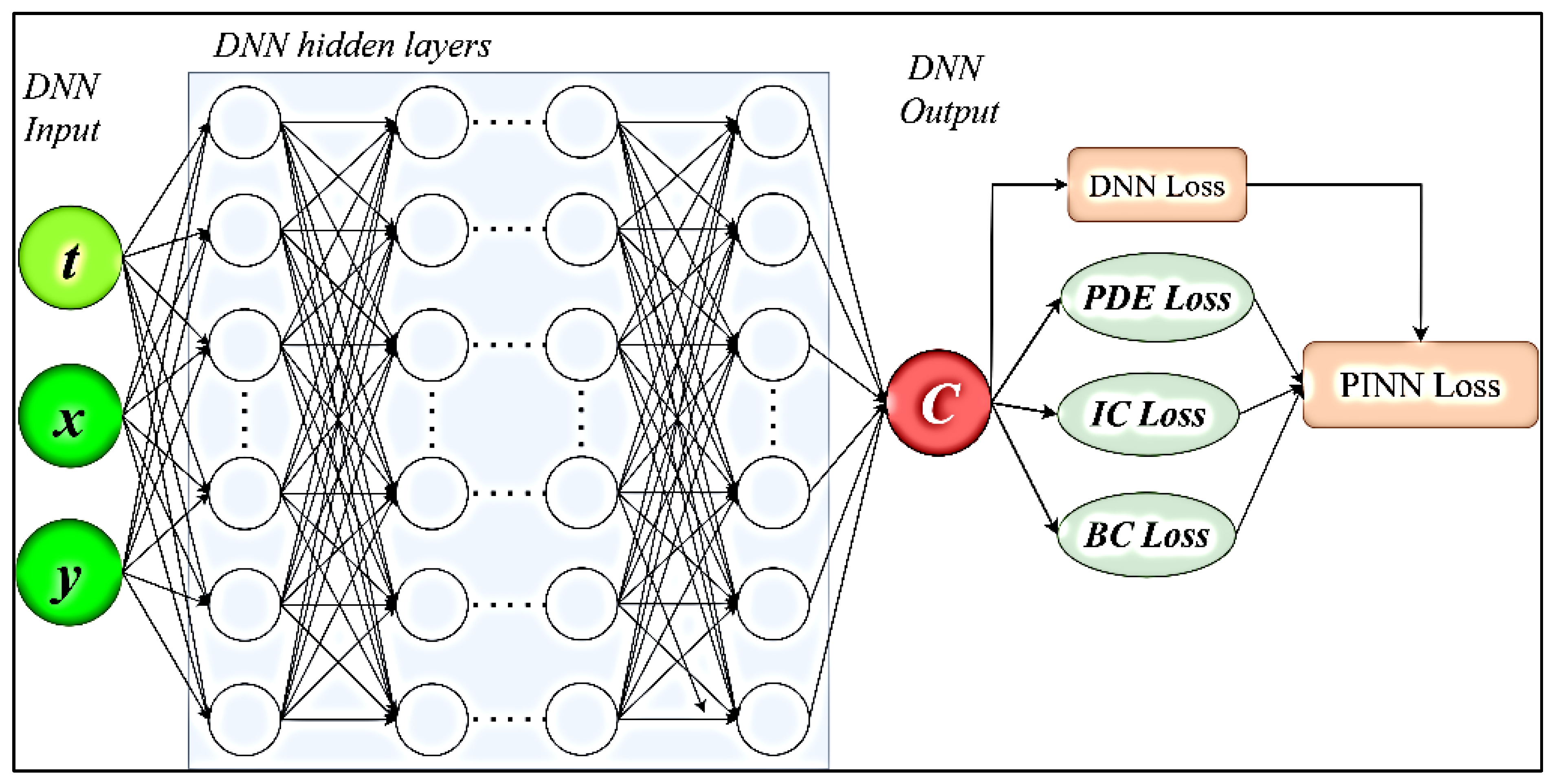
5.1. Purely Data-Driven DNN Modelling

Most PIML models are based on feed-forward neural networks with backpropagation. This consists of multiple layers, including the input layer (set of input variables, called independent variables), the output layers (dependent variables), and the hidden layers between the input and output layers. In a supervised training algorithm with known data, the DNN is trained iteratively to minimise the loss function. Loss is the difference between the ground truth (known value) and the predicted value. This difference can be mathematically defined in a variety of ways (e.g., mean squared error (MSE), mean absolute error (MAE), root mean squared error (RMSE) based on the performance and the application [125]:

$$MS{E}_{DNN}=\frac{1}{n}{{\displaystyle \sum _{i=1}^n\left[c_{gt}-{\widehat{c}}_p\right]}}^2$$

(25)

where $c_{gt}$ is the known ground truth moisture concentration values, $c_p$ is the predicted moisture concentration values, and $n$ is the spatiotemporal domain size. The aim of the pure ddata-driven DNN model is to train the neural network parameters ($\theta :=\left(W, b\right)$) to minimise the loss function ($MS{E}_{DNN}$), so the DNN training completely relies on the dataset used for training. Better accuracy can be expected if sufficient datasets are available.

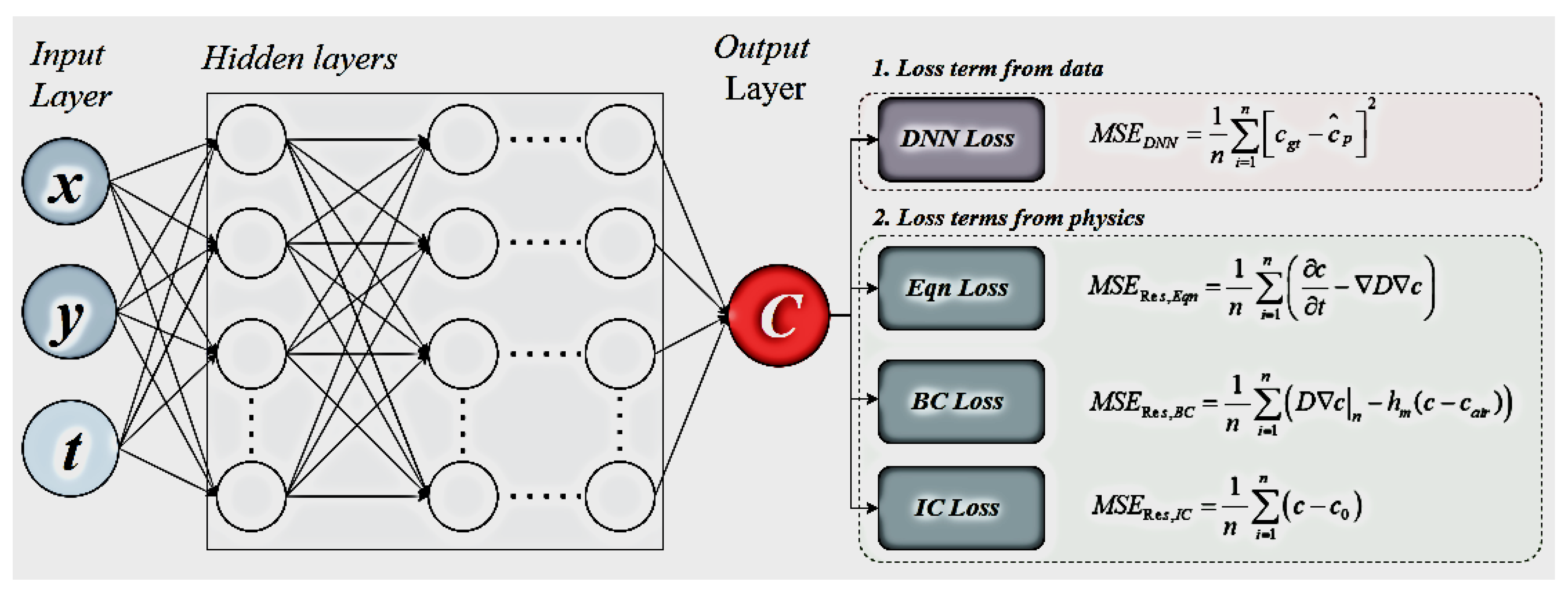
5.2. Physics-Encoded PIML MODEL

In the PIML framework, the additional loss terms from physics are coupled with the loss function defined in Equation (26). For illustration, MSE of the residuals of Fick’s diffusion governing law, boundary condition, and initial conditions for mass transfer model during drying can be encoded to the DNN by the following expressions.

The residual of the governing equation (Fick’s second law of diffusion) is as follows:

$$MS{E}_{\mathit{Re}s,Eqn}=\frac{1}{n_{}}{\displaystyle \sum _{i=1}^{n_{}}\left(\frac{\partial c}{\partial t}-\nabla D\nabla c\right)}$$

(26)

The residual of the boundary condition (convective mass transfer at the boundary) can be written as follows:

$$MS{E}_{\mathit{Re}s,BC}=\frac{1}{n_{}}{\displaystyle \sum _{i=1}^{n_{}}\left({\left.D\nabla c\right|}_n-h_m(c-c_{air})\right)}$$

(27)

The residual of the initial condition (moisture content at the fresh condition) can be expressed as follows:

$$MS{E}_{\mathit{Re}s,IC}=\frac{1}{n_{}}{\displaystyle \sum _{i=1}^{n_{}}\left(c-c_0\right)}$$

(28)

where $c$ is moisture concentration, $D$ is diffusivity, $t$ is drying time, $h_m$ is the mass transfer coefficient, and $c_{air}$ and $c_0$ are moisture concentration of the air and initial state, respectively.

In order to develop the PIML for mass transfer during drying, the residual loss terms from the physics conditions discussed above are required to couple with the pure data-driven DNN loss function.

$$MS{E}_{Total}=MS{E}_{DNN}+MS{E}_{\mathit{Re}s,Eqn}+MS{E}_{\mathit{Re}s,BC}+MS{E}_{\mathit{Re}s,IC}$$

(29)

$$MS{E}_{Total}=\frac{1}{n}\left[{{\displaystyle \sum _{i=1}^n\left[c_{gt}-{\widehat{c}}_p\right]}}^2+{\displaystyle \sum _{i=1}^{n_{}}\left(\frac{\partial c}{\partial t}-\nabla D\nabla c\right)}+{\displaystyle \sum _{i=1}^{n_{}}\left({\left.D\nabla c\right|}_n-h_m(c-c_{air})\right)}+{\displaystyle \sum _{i=1}^{n_{}}\left(c-c_0\right)}\right]$$

(30)

The schematic representation of PIML with mass-transfer-related physics during drying is illustrated in Figure 6. Now, the neural network parameters ($\theta :=\left(W, b\right)$) are trained iteratively to minimise the total loss function ($MS{E}_{Total}$). Therefore, the predictions from the well-trained model obey the dataset, as well as embedded physics equations and conditions.

Even though both the Python and MATLAB programming languages can be successfully used to develop PIML models, Python has received considerable demand due to the availability of open-source code and libraries. Haghighat and Juanes [126] published a PIML model developing steps through a special application programming interface (API) called SciANN. Nascimento et al. [127] gave a comprehensive demonstration of the implementation of PIML models to solve typical PDEs. Moreover, Bai et al. [128] published source code development steps for solid mechanics problems. Both of them used Python and provided source code in the GitHub open-source community.

6. Conjugation of Airflow in the Drying Model

The conjugation of airflow distribution across the dryer and around the products needs to be taken into consideration when developing an accurate drying model. During convective drying, the turbulent airflow inside the dryer creates huge, non-uniform air distribution around products (Figure 3a). This non-uniform airflow significantly changes the local heat and mass transfer coefficients of air across the products. The uneven distribution of heat and mass transfer coefficients significantly alters the drying kinetics, as well as the rate of drying. However, most existing theoretical drying models are developed without considering the airflow distribution and assuming constant characteristics for the convective air, considering a user-defined constant heat and mass transfer coefficient. This assumption may lead to inaccurate prediction of drying kinetics. The conjugation of airflow distribution with the transport model is a challenging and complex task. An airflow model, for example, any computational fluid dynamics (CFD) model, can be integrated with the transport model in two different ways, and these can be referred to as the fully conjugate model and the semi-conjugate model. Integration of CFD directly with the heat and mass balance equations in the transport model is called the fully conjugate model and is the more appropriate approach. Alternatively, the CFD model can be integrated with the transport model through boundary conditions, and this model is referred to as a semi-conjugate model [32]. To develop a conjugate drying model, extensive CFD analysis is required. In this case, different turbulence models, such as the k-ω model, k-ε model, algebraic Y-plus (SPF) model, L-VEL model, low-Reynolds-number k-ε mode (AKN), and SST model, can be used to integrate CFD with the drying model. These models can be solved by using Reynolds-averaged Navier–Stokes (RANS) equations [129].

Among these turbulence models, the k-ω model has been widely used due to its simplicity and accurate prediction capability. Khan et al. [32] developed a semi-conjugate model to predict the spatial distribution of airflow across the products during intermittent microwave convective drying (IMCD). A k-ω turbulence model was integrated with the drying model (simultaneous heat and mass transport) and volumetric heating (electromagnetic) model, as shown in Figure 7. Well-known physics, including Fick’s second law of mass transport, Fourier’s law of heat transfer, Lambert’s law for volumetric (microwave) heating, and the Navier–Stokes equation for CFD analysis, was used to address the simultaneous heat, mass, and momentum transport process with volumetric heating. The model was solved using COMSOL Multiphysics commercial software.

The authors found that spatial distribution of heat and mass transfer significantly affects drying kinetics. They argued that a drying model that does not have CFD integrated may overpredict drying kinetics [32]. A similar study was conducted by Defraeye et al. [130]. Although their model is able to predict convective heat and mass transfer phenomena, they did not consider the original drying processes, such as the simultaneous heat and mass transfer process. To address this gap, Defraeye and Radu [131] recently developed a CFD-integrated convective drying model. They observed that complex airflow distribution significantly affects drying kinetics. The aforementioned studies were conducted based on purely physics-based modelling. PIML-based airflow modelling could be an exciting approach to predict airflow distribution during drying. Although few attempts have been made to develop PIML-based airflow modelling for other engineering applications [132,133], no PIML-based conjugated model for drying applications is available in the literature. Therefore, future research is recommended to address this research gap.

7. Challenges to Develop Drying Models

7.1. Challenges to Capturing Local Scale Information

As mentioned earlier, drying is a complex, multifaceted problem [44]. This complex drying becomes more complicated when it is subjected to drying food materials. One of the major challenges to developing a comprehensive drying model is the consideration of the multiscale features of the domain. Food materials, particularly plant-based ones, contain multiscale heterogeneous structures (Figure 4). Mathematically addressing the multiphase transport phenomena on both the micro- and macro scales is one of the challenging tasks for drying modelling. This is because the transport phenomena and the underlying physics are different on different scales. For example, moisture located in the microscale (inside the cell) migrates through periodic cell rupture, as well as continuous diffusion [23,58]. On the other hand, the transport of free water from the macroscale domain is simply through diffusion. These different moisture transport characteristics at various scales make the overall problem very complex; therefore, mathematically addressing this problem is one of the biggest challenges in drying modelling. One of the major difficulties of multiscale modelling is capturing the microscale information and upscale to the macroscale. Different approaches, including homogenisation, Heterogeneous multiscale modelling (HMM) and equation-free are very well-known approaches that have been widely used to upscale or downscale the local scale (microscale) information to global scale (macroscale) or vice versa for multiscale modelling. Homogenisation can be used only for upscaling the local scale information to the global scale; however, this approach cannot be utilised to downscale the global scale information, for instance, macroscale heat transfer to the local scale. In this case, HMM approach is the most effective concurrent approach for concurrently upscaling and downscaling the local scale and global scale information during drying. The details of the multiscale modelling strategies can be found in this publication [67].

7.2. Structural Heterogeneities and Associated Microscale Properties

One of the main complexities of drying modelling, particularly food drying modelling, is associated with the heterogeneous microstructural elements of food materials. As mentioned earlier, plant-based food materials are multiscale in nature [134], and contain irregular cellular structures (Figure 4); different cells have their unique cellular properties, such as diffusivity, permeability, thermal conductivity, and specific heat capacity. These diverse cellular properties govern the whole transport process from micro- to macroscale and change with drying time. These cellular properties are extraordinarily important for numerical modelling, particularly multiscale modelling, particularly, multiscale modelling, designing the optimal dried food products, and optimising the quality attributes of the products. For instance, micromechanical properties, such as elastic modulus, hardness, and stiffness are the key measuring indexes of textural attributes of the dried products, which are required for designing or creating new agri-based dried food products. Investigation of the microscale properties of food materials during drying is extremely challenging, as the structure of food material and the moisture content continuously change throughout the drying processes. Moreover, the investigation of microscale properties requires extensive sophisticated experimental investigations, which are time-consuming and expensive, and facilities are mostly unavailable [135]. Although few microscale properties of fresh food materials are available in the literature for pear [136,137], tomato [138,139,140,141], onion [142], and apple [143,144], to the best of the author’s knowledge, no microscale properties of food materials during drying exist in the literature. This creates a major obstacle to advancing the field by optimising drying processes and addressing the quality attributes of the products address such research challenges, for the first time, Khan et al. [145] attempted to investigate the micromechanical properties of food materials during drying using the nanoindentation method. This study is a great new addition to the field to provide fundamental information on micro-level properties during drying time. However, performing the sophisticated experimental procedure on the microstructural elements such as on the cell wall of F&V during drying is extraordinarily difficult [146]. This is because the drying process continuously changes the shape and size of the wall. To overcome these challenges of experimental study, a prediction-based modelling approach is required. Recently, Khan et al. [146] developed a novel machine learning (ML)-based approach to characterise and predict the micromechanical properties of F&V during drying using an artificial neural network (ANN). The developed model was optimised using the genetic algorithm (GA)-based optimisation tool and validated with the experimental data. They found that the developed ML-based predictive model can accurately predict the microscale properties of different F&V [146]. However, the inherent “black box” nature of ANN challenges interpreting the actual decision-making process. Moreover, the prediction ability of purely ML-based models is often physically inconsistent and has poor generalization performance due to extrapolation or observational biases. To overcome these problems of purely ML-based models, physics-based laws (numerical derivatives) of drying processes can be integrated with ML-based algorithms. For example, Fick’s law of diffusion can be integrated with ANN algorithms to solve diffusivity. To facilitate this fundamental need, physics-informed machine learning (PIML) has emerged as a hybrid modelling paradigm that has the potential to predict the microscale properties during drying.

7.3. Shrinkage of the Products during Drying

Shrinkage is an important phenomenon that happens during drying. During drying, the viscoelastic matrix contracts due to the moisture loss from the different cellular compartments of the heterogeneous food materials. The contraction of the viscoelastic matrix causes a large amount of deformation. The deformation of the products not only affects their quality attributes but also the heat and mass transport processes. Therefore, accounting for deformation in drying modelling is crucial to accurately predict drying kinetics and optimise the products’ quality. Most existing theoretical food-drying models have been developed without considering global deformation (shrinkage) due to the extreme complexities of mathematically formulating the actual shrinkage phenomena. The main difficulty with developing a mechanistic model is the unavailability of the characteristic data of food materials and their corresponding physics. For example, food materials, particularly fruits and vegetables, are truly viscoelastic materials [147,148]. However, the existing literature considered food materials to be elastic or hyperelastic materials; therefore, the neo-Hookean model (theory) was used to address shrinkage phenomena during drying [15]. Although the model is able to predict the deformation of elastic materials at the macroscale, a realistic understanding of deformation in food materials cannot be achieved. The existing models were developed by considering the inappropriate assumption (food materials are purely elastic material) mainly due to the inability of the theory to mathematically express the viscoelastic behaviour of food materials during drying. Moreover, the existing deformation model was developed considering uniform deformation, whereas food materials exhibit anisotropic deformation. To address the anisotropic deformations, the structure–property relationship is required. The development of the structure–property relationship is extremely difficult, as it requires real-time fundamental information, which includes microstructural elements (cell sphericity, elongation equivalent diameter, and wall thickness) and the micromechanical properties in line with the drying processes. Due to these complexities, no structure–property relationship of food materials during drying is available in the literature. Therefore, extensive further research is recommended towards solving these major research challenges.

7.4. Modelling of Hybrid Drying

The development of theoretical (physics-based) models for describing the hybrid drying method is also challenging. Hybrid drying methods are the combination of two or three ordinary unique drying methods. For example, applying microwave energy intermittently with vacuum drying is referred to as intermittent microwave vacuum drying (IMVD). Mathematically describing and integrating all the processes in the same modelling framework is a difficult and complex task. Due to this complexity, research in this area remains almost grey, although very few theoretical models have already been developed for hybrid drying modelling, such as those for IMCD [32,149]. To advance this field, rigorous work is still required. As mentioned above, the development of purely theoretical models for hybrid drying to address the fundamental drying mechanism is extremely complex, challenging, and computationally expensive. This being the case, an advanced hybrid modelling framework combining a data-driven model, such as ML modelling, with the physics-based model (PIML) may be an exciting opportunity to mathematically address the fundamental transport process and optimise the drying processe. However, extensive research is required to develop such a complex PIML-based hybrid drying model for food drying.

7.5. PIML-Based Modelling Challenges

Even though PIML-based models can exclusively couple physics-based models with observational data for enhanced predictions, PIML also has its downsides. First, when emerging PIML for realistic applications, a massive computational cost is incurred when compared to traditional approaches. Various techniques, such as domain decomposition [150,151] and parallel implementation of PIMLs [152], have been investigated to reduce the training time with original feed-forward neural networks. In addition, hybrid multi-GPU and CPU computing provide a promising level of effectiveness for computational efficiency. However, this approach needs more work to compete with traditional computational approaches in terms of computational efficiency [106]. Second, the fully connected feed-forward neural networks often fail to converge loss terms for meaningful or correct solutions [153]. When more than one physics equation or condition is involved, loss of balance cannot easily be achieved due to the mismatch between the observational data and physics conditions. Even though self-adaptive hyperparameters for activation function [154] and loss weights [106,155] have shown better progress for PIML models, these are case-sensitive. Recently, changing the neural network base model from a feed-forward neural network to a graph neural network (GNN) has shown better capabilities for complex systems with unstructured data; however, the approach requires more research [106].

8. Conclusions

Knowledge of the simultaneous heat, mass, and momentum transport phenomena during drying is important to optimise the drying process and drying time and enhance energy efficiency. Enormous effort has been spent on understanding the actual drying process through experimental study and numerical modelling. As the experimental studies are product- and process-dependent and unable to provide the actual drying process, numerical modelling is the most effective tool to provide better insights into drying processes. Developing a purely physics-based model is very challenging and computationally intensive. PIML-based modelling has great potential to overcome the challenges of fundamental drying models. In this study, various aspects of drying processes, their working mechanisms, mathematical models of transport processes, and the potential of PIML have been broadly discussed. To develop a PIML-based property prediction model, the problem first needs to be defined by a neural network architecture. Then, it can be integrated with the relevant physics (PDE) of the problem through a combined loss function. Finally, numerical implementation needs to be performed for model training, testing, and validation. One of the major challenges of PIML modelling is to properly couple the multiphysics equations with a feed-forward neural network. If it is necessary to solve more than one physics equation or condition, loss of balance cannot easily be achieved due to the mismatch between the observational data and physics conditions. Even though the self-adaptive hyperparameters for activation function and loss weights have shown better progress for PIML models, these are case-sensitive. This problem can be minimised by changing the neural network base model from a feed-forward neural network to a GNN, which has better capabilities for solving complex systems with unstructured data. Besides PIML, other challenges include the unavailability of microscale properties, which creates a major bottleneck to developing fine-scale (micro- or multiscale) modelling. To overcome these challenges, further research is recommended. Overall, it is expected that the potential information in this paper will be highly beneficial for future advancements in drying research.

References

1. Air-Dried Food Market Size, Global Industry Report, 2020–2027. 2020. Report No: GVR-4-68038-513-7. Available online: https://www.grandviewresearch.com/industry-analysis/air-dried-food-market (accessed on 18 September 2022).
2. Khan, M.I.H.; Joardder, M.U.H.; Kumar, C.; Karim, M.A. Multiphase porous media modelling: A novel approach to predicting food processing performance. Crit. Rev. Food Sci. Nutr. 2018, 58, 528–546. [Google Scholar]
3. Rzig, R.; Khedher, N.B.; Nasrallah, S.B. A 3-D numerical heat and mass transfer model for simulating the vibration effects on drying process. Heat Transf.—Asian Res. 2017, 46, 1204–1221. [Google Scholar] [CrossRef]
4. Jomaa, W.; Puiggali, J.R. Drying of shrinking materials: Modellings with shrinkage velocity. Dry. Technol. 1991, 9, 1271–1293. [Google Scholar] [CrossRef]
5. Kiranoudis, C.T.; Tsami, E.; Maroulis, Z.B.; Marinos-Kouris, D. Drying kinetics of some fruits. Dry. Technol. 1997, 15, 1399–1418. [Google Scholar]
6. Putranto, A.; Chen, X.D.; Webley, P.A. Modeling of drying of food materials with thickness of several centimeters by the reaction engineering approach (REA). Dry. Technol. 2011, 29, 961–973. [Google Scholar]
7. Ben Mabrouk, S.; Benali, E.; Oueslati, H. Experimental study and numerical modelling of drying characteristics of apple slices. Food Bioprod. Process. 2012, 90, 719–728. [Google Scholar] [CrossRef]
8. Kaya, A.; Aydın, O.; Dincer, I. Experimental and numerical investigation of heat and mass transfer during drying of Hayward kiwi fruits (Actinidia Deliciosa Planch). J. Food Eng. 2008, 88, 323–330. [Google Scholar] [CrossRef]
9. Khan, M.I.H.; Pham, D.N.; Karim, A. Theoretical and experimental investigation of temperature and moisture distributions and changes in nutritional quality during intermittent microwave convective drying. In Proceedings of the 21st International Drying Symposium, Editorial Universitat Politecnica de Valencia, Valencia, Spain, 11–14 September 2018; 2018; pp. 553–560. [Google Scholar] [CrossRef] [Green Version]
10. Golestani, R.; Raisi, A.; Aroujalian, A. Mathematical Modeling on Air Drying of Apples Considering Shrinkage and Variable Diffusion Coefficient. Dry. Technol. 2013, 31, 40–51. [Google Scholar] [CrossRef]
11. Kumar, C.; Millar, G.J.; Karim, M.A. Effective Diffusivity and Evaporative Cooling in Convective Drying of Food Material. Dry. Technol. 2014, 33, 227–237. [Google Scholar] [CrossRef] [Green Version]
12. Fowler, A.J.; Bejan, A. The effect of shrinkage on the cooking of meat. Int. J. Heat Fluid Flow 1991, 12, 375–383. [Google Scholar]
13. Khan, M.; Kumar, C.; Joardder, M.U.H.; Karim, M.A. Determination of appropriate effective diffusivity for different food materials. Dry. Technol. 2017, 35, 335–346. [Google Scholar] [CrossRef]
14. Datta, A.K. Porous media approaches to studying simultaneous heat and mass transfer in food processes. I: Problem formulations. J. Food Eng. 2007, 80, 80–95. [Google Scholar]
15. Gulati, T.; Datta, A.K. Mechanistic understanding of case-hardening and texture development during drying of food materials. J. Food Eng. 2015, 166, 119–138. [Google Scholar] [CrossRef]
16. Mercier, S.; Marcos, B.; Moresoli, C.; Mondor, M.; Villeneuve, S. Modeling of internal moisture transport during durum wheat pasta drying. J. Food Eng. 2014, 124, 19–27. [Google Scholar]
17. Batuwatta-Gamage, C.P.; Rathnayaka, C.M.; Karunasena, H.C.P.; Wijerathne, W.D.C.C.; Jeong, H.; Welsh, Z.G.; Karim, M.A.; Gu, Y.T. A physics-informed neural network-based surrogate framework to predict moisture concentration and shrinkage of a plant cell during drying. J. Food Eng. 2022, 332, 111137. [Google Scholar] [CrossRef]
18. Karniadakis, G.E.; Kevrekidis, I.G.; Lu, L.; Perdikaris, P.; Wang, S.; Yang, L. Physics-informed machine learning. Nat. Rev. Phys. 2021, 3, 422–440. [Google Scholar] [CrossRef]
19. Raissi, M.; Yazdani, A.; Karniadakis, G.E. Hidden fluid mechanics: Learning velocity and pressure fields from flow visualizations. Science 2020, 367, 1026–1030. [Google Scholar] [CrossRef]
20. Raissi, M.; Perdikaris, P.; Karniadakis, G.E. Physics-informed neural networks: A deep learning framework for solving forward and inverse problems involving nonlinear partial differential equations. J. Comput. Phys. 2019, 378, 686–707. [Google Scholar] [CrossRef]
21. Khan, M.I.H.; Karim, M. Cellular water distribution, transport, and its investigation methods for plant-based food material. Food Res. Int. 2017, 99, 1–14. [Google Scholar] [CrossRef] [Green Version]
22. Khan, M.I.H.; Wellard, R.M.; Nagy, S.A.; Joardder, M.U.H.; Karim, M.A. Investigation of bound and free water in plant-based food material using NMR T2 relaxometry. Innov. Food Sci. Emerg. Technol. 2016, 38, 252–261. [Google Scholar]
23. Khan, M.I.H.; Farrell, T.; Nagy, S.A.; Karim, M.A. Fundamental Understanding of Cellular Water Transport Process in Bio-Food Material during Drying. Sci. Rep. 2018, 8, 15191. [Google Scholar] [CrossRef] [PubMed] [Green Version]
24. Kumar, C.; Joardder, M.U.H.; Farrell, T.W.; Karim, M.A. Multiphase porous media model for intermittent microwave convective drying (IMCD) of food. Int. J. Therm. Sci. 2016, 104, 304–314. [Google Scholar] [CrossRef]
25. Hamraoui, A.; Nylander, T. Analytical Approach for the Lucas–Washburn Equation. J. Colloid Interface Sci. 2002, 250, 415–421. [Google Scholar]
26. Aguilera, J.M.; Michel, M.; Mayor, G. Fat Migration in Chocolate: Diffusion or Capillary Flow in a Particulate Solid?—A Hypothesis Paper. J. Food Sci. 2004, 69, 167–174. [Google Scholar]
27. Lucas, R. Ueber das Zeitgesetz des kapillaren Aufstiegs von Flüssigkeiten. Kolloid-Z. 1918, 23, 15–22. [Google Scholar] [CrossRef]
28. Washburn, E.W. The Dynamics of Capillary Flow. Phys. Rev. 1921, 17, 273–283. [Google Scholar]
29. Chemkhi, S.; Jomaa, W.; Zagrouba, F. Application of a Coupled Thermo-Hydro-Mechanical Model to Simulate the Drying of Nonsaturated Porous Media. Dry. Technol. 2009, 27, 842–850. [Google Scholar]
30. Fuller, E.N.; Schettler, P.D.; Giddings, J.C. A new method for prediction of binary gas-phase diffusion coefficients. Ind. Eng. Res. 1966, 58, 19–27. [Google Scholar]
31. Bolz, R.; Tuve, G. Handbook of Tables for Applied Engineering Science, 2nd ed.; CRC Press: Cleveland, OH, USA, 1976. [Google Scholar]
32. Khan, M.I.H.; Welsh, Z.; Gu, Y.; Karim, M.A.; Bhandari, B. Modelling of simultaneous heat and mass transfer considering the spatial distribution of air velocity during intermittent microwave convective drying. Int. J. Heat Mass Transf. 2020, 153, 119668. [Google Scholar] [CrossRef]
33. Bergman, T.L.; Bergman, T.L.; Incropera, F.P.; Dewitt, D.P.; Lavine, A.S. Fundamentals of Heat and Mass Transfer; John Wiley & Sons: Hoboken, NJ, USA, 2016. [Google Scholar]
34. Page, G.E. Factors Influencing the Maximum Rates of Air Drying Shelled Corn in Thin Layers; Purdue University: West Lafayette, IN, USA, 1949. [Google Scholar]
35. Lewis, W.K. The rate of drying of solid materials. Ind. Eng. Chem. 1921, 13, 427–432. [Google Scholar] [CrossRef]
36. Hendorson, S. Grain drying theory (I) temperature effect on drying coefficient. J. Agric. Eng. Res. 1961, 6, 169–174. [Google Scholar]
37. Wang, C.; Singh, R. A Single Layer Drying Equation for Rough Rice; ASAE: St. Joseph, MI, USA, 1978; No. 78-3001. [Google Scholar]
38. Chayjan, R.A.; Salari, K.; Shadidi, B. Modeling some drying characteristics of garlic sheets under semi fluidized and fluidized bed conditions. Res. Agric. Eng. 2012, 58, 73–82. [Google Scholar]
39. Toğrul, İ.T.; Pehlivan, D. Modelling of drying kinetics of single apricot. J. Food Eng. 2003, 58, 23–32. [Google Scholar] [CrossRef]
40. Queiroz, M.; Nebra, S. Theoretical and experimental analysis of the drying kinetics of bananas. J. Food Eng. 2001, 47, 127–132. [Google Scholar] [CrossRef]
41. Akpinar, E.; Midilli, A.; Bicer, Y. Single layer drying behaviour of potato slices in a convective cyclone dryer and mathematical modeling. Energy Convers. Manag. 2003, 44, 1689–1705. [Google Scholar] [CrossRef]
42. El-Sebaii, A.; El-Sebaii, A.A.; Aboul-Enein, S.; Ramadan, M.R.I.; El-Gohary, H.G. Empirical correlations for drying kinetics of some fruits and vegetables. Energy 2002, 27, 845–859. [Google Scholar]
43. Midilli, A.; Kucuk, H. Mathematical modeling of thin layer drying of pistachio by using solar energy. Energy Convers. Manag. 2003, 44, 1111–1122. [Google Scholar] [CrossRef]
44. Khan, M.I.H.; Sablani, S.S.; Nayak, R.; Gu, Y. Machine learning-based modeling in food processing applications: State of the art. Compr. Rev. Food Sci. Food Saf. 2022, 21, 1409–1438. [Google Scholar] [CrossRef]
45. Batista, L.M.; da Rosa, C.A.; Pinto, L.A. Diffusive model with variable effective diffusivity considering shrinkage in thin layer drying of chitosan. J. Food Eng. 2007, 81, 127–132. [Google Scholar] [CrossRef]
46. Pham, N.D.; Khan, M.; Karim, M. A mathematical model for predicting the transport process and quality changes during intermittent microwave convective drying. Food Chem. 2020, 325, 126932. [Google Scholar] [CrossRef]
47. Da Silva, W.P.; da Silva, L.D.; Nascimento, P.L. Optimization and simulation of drying processes using diffusion models: Application to wood drying using forced air at low temperature. Wood Sci. Technol. 2011, 45, 787–800. [Google Scholar] [CrossRef]
48. Telljohann, U.; Junge, K.; Specht, E. Moisture Diffusion Coefficients for Modeling the First and Second Drying Sections of Green Bricks. Dry. Technol. 2008, 26, 855–863. [Google Scholar] [CrossRef]
49. Lu, X.; Tsotsas, E.; Kharaghani, A. Drying of capillary porous media simulated by coupling of continuum-scale and micro-scale models. Int. J. Multiph. Flow 2021, 140, 103654. [Google Scholar] [CrossRef]
50. Luikov, A.V. Systems of differential equations of heat and mass transfer in capillary-porous bodies. Int. J. Heat Mass Transf. 1975, 18, 1–14. [Google Scholar] [CrossRef]
51. Whitaker, S. Simultaneous Heat, Mass, and Momentum Transfer in Porous Media: A Theory of Drying. In Advances in Heat Transfer; James, P.H., Thomas, F.I., Eds.; Elsevier: Amsterdam, The Netherlands, 1977; pp. 119–203. [Google Scholar]
52. Curcio, S. A Multiphase Model to Analyze Transport Phenomena in Food Drying Processes. Dry. Technol. 2010, 28, 773–785. [Google Scholar] [CrossRef]
53. Dhall, A.; Squier, G.; Geremew, M.; Wood, W.A.; George, J.; Datta, A.K. Modeling of Multiphase Transport during Drying of Honeycomb Ceramic Substrates. Dry. Technol. 2012, 30, 607–618. [Google Scholar] [CrossRef]
54. Perré, P.; Turner, I.W. A 3-D version of TransPore: A comprehensive heat and mass transfer computational model for simulating the drying of porous media. Int. J. Heat Mass Transf. 1999, 42, 4501–4521. [Google Scholar] [CrossRef]
55. Autengruber, M.; Lukacevic, M.; Füssl, J. Finite-element-based moisture transport model for wood including free water above the fiber saturation point. Int. J. Heat Mass Transf. 2020, 161, 120228. [Google Scholar]
56. Simo-Tagne, M.; Bennamoun, L.; Léonard, A.; Rogaume, Y. Modeling, numerical simulation and validation of a convective dryer in steady conditions: Case study of tropical woods. Int. J. Model. Simul. 2020, 40, 143–161. [Google Scholar] [CrossRef]
57. Khan, M.I.H.; Nagy, S.A.; Karim, M. Transport of cellular water during drying: An understanding of cell rupturing mechanism in apple tissue. Food Res. Int. 2018, 105, 772–781. [Google Scholar]
58. Khan, M.I.H.; Wellard, R.M.; Nagy, S.A.; Joardder, M.U.H.; Karim, M.A. Experimental investigation of bound and free water transport process during drying of hygroscopic food material. Int. J. Therm. Sci. 2017, 117, 266–273. [Google Scholar] [CrossRef]
59. Welsh, Z.G.; Khan, M.I.H.; Karim, M.A. Multiscale modeling for food drying: A homogenized diffusion approach. J. Food Eng. 2021, 292, 110252. [Google Scholar]
60. Welsh, Z.G.; Simpson, M.J.; Khan, M.I.H.; Karim, A. A multiscale approach to estimate the cellular diffusivity during food drying. Biosyst. Eng. 2021, 212, 273–289. [Google Scholar] [CrossRef]
61. Perré, P. Multiscale modeling of drying as a powerful extension of the macroscopic approach: Application to solid wood and biomass processing. Dry. Technol. 2010, 28, 944–959. [Google Scholar] [CrossRef]
62. Zadin, V.; Kasemägi, H.; Valdna, V.; Vigonski, S.; Veske, M.; Aabloo, A. Application of multiphysics and multiscale simulations to optimize industrial wood drying kilns. Appl. Math. Comput. 2015, 267, 465–475. [Google Scholar] [CrossRef]
63. Díaz, A.R.; Flores, E.I.S.; Yanez, S.J.; Vasco, D.A.; Pina, J.C.; Guzmán, C.F. Multiscale modeling of the thermal conductivity of wood and its application to cross-laminated timber. Int. J. Therm. Sci. 2019, 144, 79–92. [Google Scholar] [CrossRef]
64. Liu, L.; Wang, X.; Chen, H.; Wan, C.; Zhang, M. Numerical modeling of drying shrinkage deformation of cement-based composites by coupling multiscale structure model with 3D lattice analyses. Comput. Struct. 2017, 178, 88–104. [Google Scholar] [CrossRef]
65. Ho, Q.T.; Verboven, P.; Verlinden, B.E.; Herremans, E.; Wevers, M.; Carmeliet, J.; Nicolaï, B.M. A 3-D multiscale model for gas exchange in fruit. Plant Physiol. 2011, 155, 1158–1168. [Google Scholar]
66. Aregawi, W.A.; Abera, M.K.; Fanta, S.W.; Verboven, P.; Nicolai, B. Prediction of water loss and viscoelastic deformation of apple tissue using a multiscale model. J. Phys. Condens. Matter 2014, 26, 464111. [Google Scholar] [CrossRef]
67. Welsh, Z.; Simpson, M.J.; Khan, M.I.H.; Karim, M.A. Multiscale Modeling for Food Drying: State of the Art. Compr. Rev. Food Sci. Food Saf. 2018, 17, 1293–1308. [Google Scholar] [CrossRef] [Green Version]
68. Ritto, T.G.; Rochinha, F.A. Digital twin, physics-based model, and machine learning applied to damage detection in structures. Mech. Syst. Signal Process. 2021, 155, 107614. [Google Scholar]
69. Jordan, M.I.; Mitchell, T.M. Machine learning: Trends, perspectives, and prospects. Science 2015, 349, 255–260. [Google Scholar] [CrossRef]
70. Kumar, P.; Sinha, K.; Nere, N.K.; Shin, Y.; Ho, R.; Mlinar, L.B.; Sheikh, A.Y. A machine learning framework for computationally expensive transient models. Sci. Rep. 2020, 10, 11492. [Google Scholar] [CrossRef] [PubMed]
71. Liu, W.; Wang, Z.; Liu, X.; Zeng, N.; Liu, Y.; Alsaadi, F.E. A survey of deep neural network architectures and their applications. Neurocomputing 2017, 234, 11–26. [Google Scholar] [CrossRef]
72. Chicco, D. Ten quick tips for machine learning in computational biology. BioData Min. 2017, 10, 35. [Google Scholar] [PubMed] [Green Version]
73. Alzubaidi, L.; Zhang, J.; Humaidi, A.J.; Al-Dujaili, A.; Duan, Y.; Al-Shamma, O.; Santamaría, J.; Fadhel, M.A.; Al-Amidie, M.; Farhan, L. Review of deep learning: Concepts, CNN architectures, challenges, applications, future directions. J. Big Data 2021, 8, 53. [Google Scholar] [CrossRef]
74. Li, G.; Hari, S.K.S.; Sullivan, M.; Tsai, T.; Pattabiraman, K.; Emer, J.; Keckler, S.W. Understanding error propagation in deep learning neural network (DNN) accelerators and applications. In Proceedings of the International conference for High Performance Computing, Networking, Storage and Analysis, Denver, CO, USA, 12–17 November 2017; pp. 1–12. [Google Scholar]
75. Wu, H.; Lv, D.; Cui, T.; Hou, G.; Watanabe, M.; Kong, W. SDLV: Verification of Steering Angle Safety for Self-Driving Cars. Form. Asp. Comput. 2021, 33, 325–341. [Google Scholar] [CrossRef]
76. Cardoso, V.B.; Oliveira, A.S.; Forechi, A.; Azevedo, P.; Mutz, F.; Oliveira-Santos, T.; Badue, C.; De Souza, A.F. A Large-Scale Mapping Method Based on Deep Neural Networks Applied to Self-Driving Car Localization. In Proceedings of the 2020 International Joint Conference on Neural Networks (IJCNN), Glasgow, UK, 19–24 July 2020; pp. 1–8. [Google Scholar]
77. Dahl, G.E.; Yu, D.; Deng, L.; Acero, A. Context-Dependent Pre-Trained Deep Neural Networks for Large-Vocabulary Speech Recognition. IEEE Trans. Audio Speech Lang. Process. 2012, 20, 30–42. [Google Scholar]
78. Tachbelie, M.Y.; Abulimiti, A.; Abate, S.T.; Schultz, T. DNN-Based Speech Recognition for Globalphone Languages. In Proceedings of the ICASSP 2020–2020 IEEE International Conference on Acoustics, Speech and Signal Processing (ICASSP), Barcelona, Spain, 4–8 May 2020; pp. 8269–8273. [Google Scholar]
79. Smit, P.; Virpioja, S.; Kurimo, M. Advances in subword-based HMM-DNN speech recognition across languages. Comput. Speech Lang. 2021, 66, 101158. [Google Scholar]
80. Wang, D.; Wang, X.; Lv, S. An overview of end-to-end automatic speech recognition. Symmetry 2019, 11, 1018. [Google Scholar]
81. Nagrath, P.; Jain, R.; Madan, A.; Arora, R.; Kataria, P.; Hemanth, J. SSDMNV2: A real time DNN-based face mask detection system using single shot multibox detector and MobileNetV2. Sustain. Cities Soc. 2021, 66, 102692. [Google Scholar] [CrossRef] [PubMed]
82. Cao, N.; Chatterjee, B.; Gong, M.; Chang, M.; Sen, S.; Raychowdhury, A. A 65 nm Image Processing SoC Supporting Multiple DNN Models and Real-Time Computation-Communication Trade-Off Via Actor-Critical Neuro-Controller. In Proceedings of the 2020 IEEE Symposium on VLSI Circuits, Honolulu, HI, USA, 16–19 June 2020; pp. 1–2. [Google Scholar]
83. Yang, X.; Li, F.; Liu, H. A Survey of DNN Methods for Blind Image Quality Assessment. IEEE Access 2019, 7, 123788–123806. [Google Scholar]
84. Mallikarjuna, B.; Shrivastava, G.; Sharma, M. Blockchain technology: A DNN token-based approach in healthcare and COVID-19 to generate extracted data. Expert Syst. 2021, 39, e12778. [Google Scholar] [CrossRef] [PubMed]
85. Shi, J.; Fan, X.; Wu, J.; Chen, J.; Chen, W. DeepDiagnosis: DNN-Based Diagnosis Prediction from Pediatric Big Healthcare Data. In Proceedings of the 2018 Sixth International Conference on Advanced Cloud and Big Data (CBD), Lanzhou, China, 12–15 August 2018. [Google Scholar]
86. Shamshirband, S.; Fathi, M.; Dehzangi, A.; Chronopoulos, A.T.; Alinejad-Rokny, H. A review on deep learning approaches in healthcare systems: Taxonomies, challenges, and open issues. J. Biomed. Inform. 2021, 113, 103627. [Google Scholar] [CrossRef]
87. Jain, S.; Chauhan, R. Recognition of Handwritten Digits Using DNN, CNN, and RNN. In Advances in Computing and Data Sciences; Springer: Singapore, 2018. [Google Scholar]
88. Rismiyati; Khadijah; Nurhadiyatna, A. Deep learning for handwritten Javanese character recognition. In Proceedings of the 2017 1st International Conference on Informatics and Computational Sciences (ICICoS), Semarang, Indonesia, 15–16 November 2017. [Google Scholar]
89. Koyuncu, B.; Koyuncu, H. Handwritten Character Recognition by using Convolutional Deep Neural Network; Review. Int. J. Eng. Technol. IJET 2019, 5, 1–5. [Google Scholar]
90. Felix, A.Y.; Jesudoss, A.; Mayan, J.A. Entry and exit monitoring using license plate recognition. In Proceedings of the 2017 IEEE International Conference on Smart Technologies and Management for Computing, Communi-cation, Controls, Energy and Materials (ICSTM), Chennai, India, 2–4 August 2017. [Google Scholar]
91. Rackauckas, C.; Ma, Y.; Martensen, J.; Warner, C.; Zubov, K.; Supekar, R.; Skinner, D.; Ramadhan, A.; Edelman, A. Universal differential equations for scientific machine learning. arXiv 2020, arXiv:2001.04385. [Google Scholar]
92. Sun, Q.; Zhang, M.; Mujumdar, A.S. Recent developments of artificial intelligence in drying of fresh food: A review. Crit. Rev. Food Sci. Nutr. 2019, 59, 2258–2275. [Google Scholar]
93. Khan, M.I.H.; Sablani, S.S.; Joardder, M.U.H.; Karim, M.A. Application of machine learning-based approach in food drying: Opportunities and challenges. Dry. Technol. 2022, 40, 1051–1067. [Google Scholar] [CrossRef]
94. Martynenko, A.; Misra, N.N. Machine learning in drying. Dry. Technol. 2019, 38, 596–609. [Google Scholar] [CrossRef]
95. Fabani, M.P.; Capossio, J.P.; Román, M.C.; Zhu, W.; Rodriguez, R.; Mazza, G. Producing non-traditional flour from watermelon rind pomace: Artificial neural network (ANN) modeling of the drying process. J. Environ. Manag. 2021, 281, 111915. [Google Scholar] [CrossRef] [PubMed]
96. Demirpolat, A.B. Investigation of Mass Transfer with Different Models in a Solar Energy Food-Drying System. Energies 2019, 12, 3447. [Google Scholar]
97. Kırbaş, İ.; Tuncer, A.D.; Şirin, C.; Usta, H. Modeling and developing a smart interface for various drying methods of pomelo fruit (Citrus maxima) peel using machine learning approaches. Comput. Electron. Agric. 2019, 165, 104928. [Google Scholar] [CrossRef]
98. Islam, M.R.; Sablani, S.S.; Mujumdar, A.S. An Artificial Neural Network Model for Prediction of Drying Rates. Dry. Technol. 2003, 21, 1867–1884. [Google Scholar]
99. Qadri, O.S.; Osama, K.; Srivastava, A.K. Foam mat drying of papaya using microwaves: Machine learning modeling. J. Food Process Eng. 2020, 43, e13394. [Google Scholar] [CrossRef]
100. Ochoa-Martínez, C.I.; Ayala-Aponte, A.A. Prediction of mass transfer kinetics during osmotic dehydration of apples using neural networks. LWT—Food Sci. Technol. 2007, 40, 638–645. [Google Scholar] [CrossRef]
101. Chen, Y.; Martynenko, A. Computer vision for real-time measurements of shrinkage and color changes in blueberry convective drying. Dry. Technol. 2013, 31, 1114–1123. [Google Scholar]
102. Udomkun, P.; Nagle, M.; Argyropoulos, D.; Mahayothee, B.; Müller, J. Multi-sensor approach to improve optical monitoring of papaya shrinkage during drying. J. Food Eng. 2016, 189, 82–89. [Google Scholar] [CrossRef]
103. Iheonye, A.; Gariepy, Y.; Raghavan, V. Computer vision for real-time monitoring of shrinkage for peas dried in a fluidized bed dryer. Dry. Technol. 2019, 38, 130–146. [Google Scholar] [CrossRef]
104. Das, M.; Alic, E.; Akpinar, E.K. Detailed analysis of mass transfer in solar food dryer with different methods. Int. Commun. Heat Mass Transf. 2021, 128, 105600. [Google Scholar] [CrossRef]
105. Hernandez-Perez, J.A.; Garcıa-Alvarado, M.A.; Trystram, G.; Heyd, B. Neural networks for the heat and mass transfer prediction during drying of cassava and mango. Innov. Food Sci. Emerg. Technol. 2004, 5, 57–64. [Google Scholar] [CrossRef]
106. Shukla, K.; Xu, M.; Trask, N.; Karniadakis, G.E. Scalable algorithms for physics-informed neural and graph networks. Data-Cent. Eng. 2022, 3, e24. [Google Scholar]
107. Cai, S.; Wang, Z.; Wang, S.; Perdikaris, P.; Karniadakis, G.E. Physics-Informed Neural Networks for Heat Transfer Problems. J. Heat Transf. 2021, 143, 060801. [Google Scholar]
108. Blechschmidt, J.; Ernst, O.G. Three ways to solve partial differential equations with neural networks—A review. GAMM-Mitt. 2021, 44, e202100006. [Google Scholar]
109. Almajid, M.M.; Abu-Al-Saud, M.O. Prediction of porous media fluid flow using physics informed neural networks. J. Pet. Sci. Eng. 2022, 208, 109205. [Google Scholar] [CrossRef]
110. Weng, Y.; Zhou, D. Multiscale Physics-Informed Neural Networks for Stiff Chemical Kinetics. J. Phys. Chem. A 2022, 126, 8534–8543. [Google Scholar] [CrossRef]
111. Willard, J.; Jia, X.; Xu, S.; Steinbach, M.; Kumar, V. Integrating physics-based modeling with machine learning: A survey. arXiv 2020, arXiv:2003.04919. [Google Scholar]
112. Cai, S.; Mao, Z.; Wang, Z.; Yin, M.; Karniadakis, G.E. Physics-informed neural networks (PINNs) for fluid mechanics: A review. Acta Mech. Sin. 2022, 37, 1727–1738. [Google Scholar] [CrossRef]
113. Jagtap, A.D.; Mao, Z.; Adams, N.; Karniadakis, G.E. Physics-informed neural networks for inverse problems in supersonic flows. J. Comput. Phys. 2022, 466, 111402. [Google Scholar] [CrossRef]
114. Bai, Y.; Chen, W.; Chen, J.; Guo, W. Deep learning methods for solving linear inverse problems: Research directions and paradigms. Signal Process. 2020, 177, 107729. [Google Scholar] [CrossRef]
115. Lin, T.; Wang, Z.; Wang, W.; Sui, Y. A neural network-based algorithm for high-throughput characterisation of viscoelastic properties of flowing microcapsules. Soft Matter 2021, 17, 4027–4039. [Google Scholar]
116. Ongie, G.; Jalal, A.; Metzler, C.A.; Baraniuk, R.G.; Dimakis, A.G.; Willett, R. Deep learning techniques for inverse problems in imaging. IEEE J. Sel. Areas Inf. Theory 2020, 1, 39–56. [Google Scholar] [CrossRef]
117. He, Z.; Ni, F.; Wang, W.; Zhang, J.A. physics-informed deep learning method for solving direct and inverse heat conduction problems of materials. Mater. Today Commun. 2021, 28, 102719. [Google Scholar] [CrossRef]
118. Laubscher, R. Simulation of multi-species flow and heat transfer using physics-informed neural networks. Phys. Fluids 2021, 33, 087101. [Google Scholar] [CrossRef]
119. Niaki, S.A.; Haghighat, E.; Campbell, T.; Poursartip, A.; Vaziri, R. Physics-informed neural network for modelling the thermochemical curing process of composite-tool systems during manufacture. Comput. Methods Appl. Mech. Eng. 2021, 384, 113959. [Google Scholar]
120. Laubscher, R.; Rousseau, P. Application of a mixed variable physics-informed neural network to solve the incompressible steady-state and transient mass, momentum, and energy conservation equations for flow over in-line heated tubes. Appl. Soft Comput. 2022, 114, 108050. [Google Scholar] [CrossRef]
121. Zhang, W.; al Kobaisi, M. On the Monotonicity and Positivity of Physics-Informed Neural Networks for Highly Anisotropic Diffusion Equations. Energies 2022, 15, 6823. [Google Scholar] [CrossRef]
122. Liu, M.; Liang, L.; Sun, W. A generic physics-informed neural network-based constitutive model for soft biological tissues. Comput. Methods Appl. Mech. Eng. 2020, 372, 113402. [Google Scholar]
123. Taghizadeh, E.; Byrne, H.M.; Wood, B.D. Explicit physics-informed neural networks for nonlinear closure: The case of transport in tissues. J. Comput. Phys. 2022, 449, 110781. [Google Scholar] [CrossRef]
124. Arzani, A.; Wang, J.-X.; D’Souza, R.M. Uncovering near-wall blood flow from sparse data with physics-informed neural networks. Phys. Fluids 2021, 33, 071905. [Google Scholar] [CrossRef]
125. Kowalczyk, D.; Baraniak, B. Effect of candelilla wax on functional properties of biopolymer emulsion films—A comparative study. Food Hydrocoll. 2014, 41, 195–209. [Google Scholar] [CrossRef]
126. Haghighat, E.; Juanes, R. SciANN: A Keras/TensorFlow wrapper for scientific computations and physics-informed deep learning using artificial neural networks. Comput. Methods Appl. Mech. Eng. 2021, 373, 113552. [Google Scholar] [CrossRef]
127. Nascimento, R.G.; Fricke, K.; Viana, F.A.C. A tutorial on solving ordinary differential equations using Python and hybrid physics-informed neural network. Eng. Appl. Artif. Intell. 2020, 96, 103996. [Google Scholar]
128. Bai, J.; Jeong, H.; Batuwatta-Gamage, C.P.; Xiao, S.; Wang, Q.; Rathnayaka, C.M.; Alzubaidi, L.; Liu, G.R.; Gu, Y. An introduction to programming Physics-Informed Neural Network-based computational solid mechanics. arXiv 2022, arXiv:2210.09060. [Google Scholar]
129. Defraeye, T.; Verboven, P.; Nicolai, B. CFD modelling of flow and scalar exchange of spherical food products: Turbulence and boundary-layer modelling. J. Food Eng. 2013, 114, 495–504. [Google Scholar] [CrossRef] [Green Version]
130. Defraeye, T.; Herremans, E.; Verboven, P.; Carmeliet, J.; Nicolai, B. Convective heat and mass exchange at surfaces of horticultural products: A microscale CFD modelling approach. Agric. For. Meteorol. 2012, 162, 71–84. [Google Scholar] [CrossRef] [Green Version]
131. Defraeye, T.; Radu, A. Insights in convective drying of fruit by coupled modeling of fruit drying, deformation, quality evolution and convective exchange with the airflow. Appl. Therm. Eng. 2018, 129, 1026–1038. [Google Scholar] [CrossRef]
132. Wu, J.-L.; Xiao, H.; Paterson, E. Physics-informed machine learning approach for augmenting turbulence models: A comprehensive framework. Phys. Rev. Fluids 2018, 3, 074602. [Google Scholar] [CrossRef] [Green Version]
133. Wang, J.-X.; Wu, J.-L.; Xiao, H. Physics-informed machine learning approach for reconstructing Reynolds stress modeling discrepancies based on DNS data. Phys. Rev. Fluids 2017, 2, 034603. [Google Scholar] [CrossRef]
134. Rahman, M.M.; Joardder, M.U.; Khan, M.I.H.; Pham, N.D.; Karim, M.A. Multi-scale model of food drying: Current status and challenges. Crit. Rev. Food Sci. Nutr. 2018, 58, 858–876. [Google Scholar] [CrossRef] [PubMed] [Green Version]
135. Khan, M.I.H.; Rahman, M.M.; Karim, M.A. Recent advances in micro-level experimental investigation in food drying technology. Dry. Technol. 2020, 38, 557–576. [Google Scholar] [CrossRef]
136. Kozioł, A.; Cybulska, J.; Pieczywek, P.M.; Zdunek, A. Changes of pectin nanostructure and cell wall stiffness induced in vitro by pectinase. Carbohydr. Polym. 2017, 161, 197–207. [Google Scholar] [CrossRef] [PubMed]
137. Zdunek, A.; Kozioł, A.; Cybulska, J.; Lekka, M.; Pieczywek, P.M. The stiffening of the cell walls observed during physiological softening of pears. Planta 2016, 243, 519–529. [Google Scholar]
138. Zdunek, A.; Kurenda, A. Determination of the elastic properties of tomato fruit cells with an atomic force microscope. Sensors 2013, 13, 12175–12191. [Google Scholar] [PubMed] [Green Version]
139. Wang, C.; Pritchard, J.; Thomas, C. Investigation of the mechanics of single tomato fruit cells. J. Texture Stud. 2006, 37, 597–606. [Google Scholar] [CrossRef]
140. Wang, C.; Wang, L.; Thomas, C. Modelling the mechanical properties of single suspension-cultured tomato cells. Ann. Bot. 2004, 93, 443–453. [Google Scholar] [CrossRef] [PubMed] [Green Version]
141. Dintwa, E.; Jancsók, P.; Mebatsion, H.K.; Verlinden, B.; Verboven, P.; Wang, C.X.; Thomas, C.R.; Tijskens, E.; Ramon, H.; Nicolaï, B. A finite element model for mechanical deformation of single tomato suspension cells. J. Food Eng. 2011, 103, 265–272. [Google Scholar] [CrossRef]
142. Xi, X.; Kim, S.H.; Tittmann, B. Atomic force microscopy based nanoindentation study of onion abaxial epidermis walls in aqueous environment. J. Appl. Phys. 2015, 117, 024703. [Google Scholar] [CrossRef]
143. Cárdenas-Pérez, S.; Chanona-Pérez, J.J.; Méndez-Méndez, J.V.; Calderón-Domínguez, G.; López-Santiago, R.; Arzate-Vázquez, I. Nanoindentation study on apple tissue and isolated cells by atomic force microscopy, image and fractal analysis. Innov. Food Sci. Emerg. Technol. 2016, 34, 234–242. [Google Scholar] [CrossRef]
144. Cárdenas-Pérez, S.; Méndez-Méndez, J.V.; Chanona-Pérez, J.J.; Zdunek, A.; Güemes-Vera, N.; Calderón-Domínguez, G.; Rodríguez-González, F. Prediction of the nanomechanical properties of apple tissue during its ripening process from its firmness, color and microstructural parameters. Innov. Food Sci. Emerg. Technol. 2017, 39, 79–87. [Google Scholar] [CrossRef]
145. Khan, M.I.H.; Patel, N.; Mahiuddin, M.; Karim, M.A. Characterisation of mechanical properties of food materials during drying using nanoindentation. J. Food Eng. 2021, 291, 110306. [Google Scholar]
146. Khan, M.I.H.; Longa, D.; Sablani, S.S.; Gu, Y. A Novel Machine Learning–Based Approach for Characterising the Micromechanical Properties of Food Material During Drying. Food Bioprocess Technol. 2022. [CrossRef]
147. Mahiuddin, M.; Khan, M.I.H.; Kumar, C.; Rahman, M.M.; Karim, M.A. Shrinkage of food materials during drying: Current status and challenges. Compr. Rev. Food Sci. Food Saf. 2018, 17, 1113–1126. [Google Scholar] [CrossRef] [PubMed] [Green Version]
148. Mahiuddin, M.; Khan, M.I.H.; Pham, N.D.; Karim, M.A. Development of fractional viscoelastic model for characterizing viscoelastic properties of food material during drying. Food Biosci. 2018, 23, 45–53. [Google Scholar] [CrossRef] [Green Version]
149. Kumar, C.; Joardder, M.U.H.; Farrell, T.W.; Karim, M.A. Investigation of intermittent microwave convective drying (IMCD) of food materials by a coupled 3D electromagnetics and multiphase model. Dry. Technol. 2018, 36, 736–750. [Google Scholar] [CrossRef]
150. Jagtap, A.D.; Karniadakis, G.E. Extended Physics-informed Neural Networks (XPINNs): A Generalized Space-Time Domain Decomposition based Deep Learning Framework for Nonlinear Partial Differential Equations. In Proceedings of the AAAI Spring Symposium: MLPS, Stanford, CA, USA, 22–24 March 2021. [Google Scholar]
151. Kharazmi, E.; Zhang, Z.; Karniadakis, G.E.M. hp-VPINNs: Variational physics-informed neural networks with domain decomposition. Comput. Methods Appl. Mech. Eng. 2021, 374, 113547. [Google Scholar] [CrossRef]
152. Shukla, K.; Jagtap, A.D.; Karniadakis, G.E. Parallel physics-informed neural networks via domain decomposition. J. Comput. Phys. 2021, 447, 110683. [Google Scholar] [CrossRef]
153. Wang, S.; Yu, X.; Perdikaris, P. When and why PINNs fail to train: A neural tangent kernel perspective. J. Comput. Phys. 2022, 449, 110768. [Google Scholar] [CrossRef]
154. Jagtap, A.D.; Kawaguchi, K.; Karniadakis, G.E. Adaptive activation functions accelerate convergence in deep and physics-informed neural networks. J. Comput. Phys. 2020, 404, 109136. [Google Scholar]
155. Hu, H.; Dey, D.; Hebert, M.; Bagnell, J.A. Learning anytime predictions in neural networks via adaptive loss balancing. In Proceedings of the AAAI Conference on Artificial Intelligence, Atlanta, GA, USA, 8–12 October 2019. [Google Scholar]
Figure 1. Schematic representation of convection air drying processes.
Energies 15 09347 g001
Figure 2. Drying kinetics as a function of moisture content.
Energies 15 09347 g002
Figure 3. Fluid flow across a cylindrical product: (a) fluid flow stream with their boundary layer formation [33]; (b) angular positions to calculate the local heat transfer coefficient [32].
Energies 15 09347 g003
Figure 4. Schematic representation of microstructural elements of food materials.
Energies 15 09347 g004
Figure 5. Schematic representation of PIML framework (here t is the drying time, x and y is the two dimensional axis, and C is liquid conentation (mol/m3)).
Energies 15 09347 g005
Figure 6. Schematic representation of PIML for mass transfer modelling during drying.
Energies 15 09347 g006
Figure 7. Schematic diagram of different physics that was used to develop a CFD integrated 3D-IMCD model [32].
Energies 15 09347 g007
Publisher’s Note: MDPI stays neutral with regard to jurisdictional claims in published maps and institutional affiliations.