High-Resolution Emissions from Wood Burning in Norway—The Effect of Cabin Emissions

Abstract

Emissions from wood burning for heating in secondary homes or cabins is an important part in the development of high-resolution emissions in specific areas. Norway is used as case study as 20% of the national wood consumption for heating occurs in cabins. Our study first shows a method to estimate emissions from cabins based on traffic data to derive cabin occupancy, which combined with heating need allows for the spatial and temporal distribution of emissions. The combination of residential (RWC) and cabin wood combustion (CWC) emissions shows large spatial and temporal differences, and a temporally “cabin population” can in areas be orders of magnitude larger than the registered population. While RWC emissions have been steadily reduced, CWC have kept relatively constant or even increased, which results in an increase in the cabin share to total heating emissions up to 25–35%. When comparing with regional emission inventories, our study shows that the gradient between rural and urban areas is not well-represented in regional inventories, which resembles a population-based distribution and does not allocate emissions in cabin municipalities. CWC emissions may become an increasing environmental concern as higher densification trends in mountain areas are observed.

1. Introduction

Residential Wood Combustion (RWC) is a myriad of individual periodic point emission sources, which are statistically treated as a diffuse source. In Norway, with a population of ca. 5.4 million inhabitants, there are over 2.5 million wood burning stoves, and over half of them are used regularly. This high number of wood burning stoves also occurs in other countries (e.g., other Nordic countries, United Kingdoms, New Zealand) and in mountain regions (e.g., Alpine region). RWC is a valuable and important energy source for heating, but is also one of the largest contributors to particle emissions, and responsible for recurrent pollution episodes in Europe and other countries (e.g., [1,2,3,4,5]). Therefore, the understanding of RWC emissions, including the spatial and temporal distribution, is crucial for air quality management and the implementation of cost-effective measures to reduce air pollution. In order to evaluate policy scenarios and their effectiveness, emission inventories need to represent the emission process as close as possible, including accurate knowledge on where and when emissions occur. However, the distribution of residential emissions in space and time poses important challenges. Knowledge and data concerning the amount of consumed wood and the type of technology are not usually available with much geographical or temporal detail. In addition, there are several influencing factors that largely affect emissions, such as variable weather and human behavior. With regards to the latter, the way the wood stove is operated will have a strong effect on emissions, and can even be more important for emissions than the type of stove. For instance, a clean stove operated in partial-load have significantly higher emissions than an old stove operated under nominal-load [6]. Moreover, heating by wood is commonly one out of several available heating options and, thus, the share of energy sources will further vary with prices and the availability of the different energy options, such as gas and electricity.

The challenges concerning the estimation of RWC emissions and their spatio-temporal distribution have brought the need for continuous evaluation of existing emission inventories and proxies to improve these emissions. One commonly used approach for the spatial distribution of emissions has been proxies-based downscaling national emissions reported by Member States to the Convention of Long-Range Transboundary Air Pollution (CLRTAP), where RWC is included in NFR (Nomenclature for Reporting) Sector Residential: Stationary (NFR Code: 1A4bi). For instance, in CAMS regional emissions, the spatial distribution of emissions from the residential sector is done by using total population for light or medium fuels, rural population for coal and heavy liquid fuel, and wood use maps based on population density and wood demand and supply functions for biomass [7]. The use of population as ancillary data has been intensively discussed in the literature, as emissions may be overallocated in densely populated areas (e.g., [8,9]). In addition, studies highlight that spatial proxies typically used to place RWC in one area or region are hardly transferable to other areas than those where they were generated for, or they are highly inaccurate over large areas (e.g., [8,10,11]).

Local knowledge is essential to understanding emissions and developing the most accurate proxies for their spatio-temporal distribution. This needs to be done in a way that they resemble as close as possible pure bottom-up approaches, where emissions are calculated at the individual source level and, therefore, have precisely defined the spatial allocation. In the last decades, several studies have focused on the development and analysis of RWC emissions for specific countries. For instance, Paunu et al. [9] analyze the spatial distribution of RWC emissions in Nordic countries. Even though one would expect Sweden, Denmark, Norway and Finland to hold many similarities concerning wood burning activity, important differences in the predominant wood burning technology (boilers vs. wood stoves) and even the location (main distribution in suburbs vs. activity in urban areas) make the most suitable proxies for these countries different. One of the most challenging aspects for developing spatial proxies for residential emissions is to predict the fuel mix. In Norway, electricity is the main source of heating followed by wood, and other fuels only represent a minor part of the energy mix. In Poland, for instance, the main energy sources for space and water heating are hard coal followed by natural gas, wood and other minor sources. The identification of the different energy sources for heating at high-resolution represents one of the biggest challenges in these countries. Bun et al. [12] developed a high-resolution spatial emission inventory for greenhouse gas emissions in Poland and, in the case of residential emissions, they use population data along with information on access to energy sources, percentage of area equipped with central heating and data on the amount of heat energy provided to households. Similarly, Gawuc et al. [13] also developed an air pollutant emission inventory for RWC in Poland based on building data including characteristics that define their insulation factor, energy demand based on the heating degree day, the fuel mix, gas usage for heating, heat distribution network and access to heat distribution networks.

Our study considers one aspect beyond the spatial and temporal distribution of emissions from RWC, which is the use of wood burning for heating in secondary homes or cabins (cabin wood combustion; CWC, in this study), and discusses the relevance for regional emission inventories. CWC emissions are also included within the NFR Sector Residential: Stationary (1A4bi), although they are not commonly treated separately in regional inventories. Norway is used as case study as Norwegians spend less than 2% of their time at cabins but, according to the national statistics [14], over 20% of the total wood consumed occur there. Around 36% of the households in Norway have access to a cabin, the usage of which is around 31 nights on average with large variations [15,16]. Cabins are spread out over most of the Norwegian geography, and they have different building properties that often relate to their geographical location, along the coast or at the mountain.

In Norway, RWC emissions are estimated with the MetVed model, which is based on several high-resolution data-sets including dwelling number and type, wood and energy consumption, available heating technology, location of RWC chimneys and meteorology [17]. However, the proxies used for the distribution of RWC emissions are not directly transferable to emissions from CWC as, in the latter, emissions from a temporal “cabin population” needs to be determined for the different types of cabins. Other available models to distribute emissions from RWC use a weighting factor for wood combustion per building group, and in the case of holiday house they assigned 0.2, assuming to be occupied only part of the year and mostly during warmer periods [18]. This manuscript presents a novel method to estimate CWC, where both the spatial and temporal distribution largely differ from RWC. The estimation of the “cabin population” is based on determining the excess traffic in areas characterized by high density of cabins. Both RWC and CWC emissions are compared and benchmarked with CAMS regional emissions for residential heating to analyze the implications of a high share of CWC for total and urban emissions. Moreover, while, in the past, cabins were predominantly made up of simple structures and largely dispersed, our study shows how new cabin development involves the creation of large cabin settlements.

The methods and results presented in this study are especially relevant for other countries and regions (e.g., Alpine regions) with intense wood burning activity and a high share of cabins. For instance, in the Nordic countries, where the cabin stock is estimated to be around 75 per 1000 inhabitants. Moreover, the proxies can be used for other activities that entail a significant flow of population from their residence, such as energy consumption during holidays or associated with tourism activities.

2. Methodology

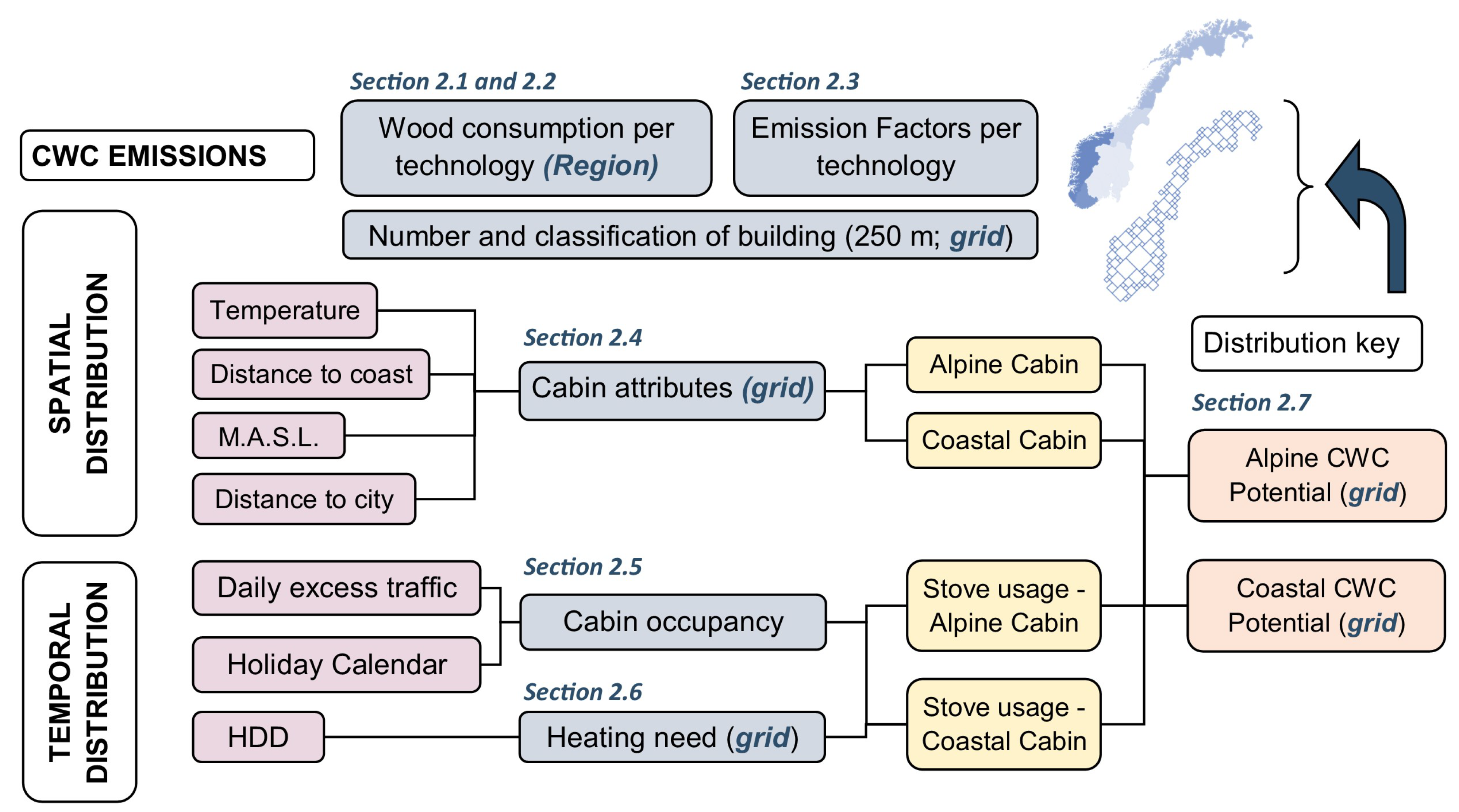
This section presents and analyses the input data used to estimate emissions and distribute them at high spatio-temporal resolution, along with the proxies to determine cabin occupancy and heating needs to, thereafter, estimate emissions. As the methodology to estimate high-resolution emissions from RWC is described in detail in [17], this section has a stronger focus on the methodological aspects concerning high-resolution emissions from CWC, also simplified in Figure 1).

2.1. Wood Consumption for Heating

The amount of wood consumed each year is estimated based on the responses to the Travel and Holiday Surveys run by Statistics Norway on a quarterly basis, where each survey covers the preceding 12 months. The annual wood consumption for heating is then obtained by the average of five consecutive quarterly surveys [14]. The sampling of the survey is drawn at a nationwide level and is considered representative for all 11 Norwegian counties. 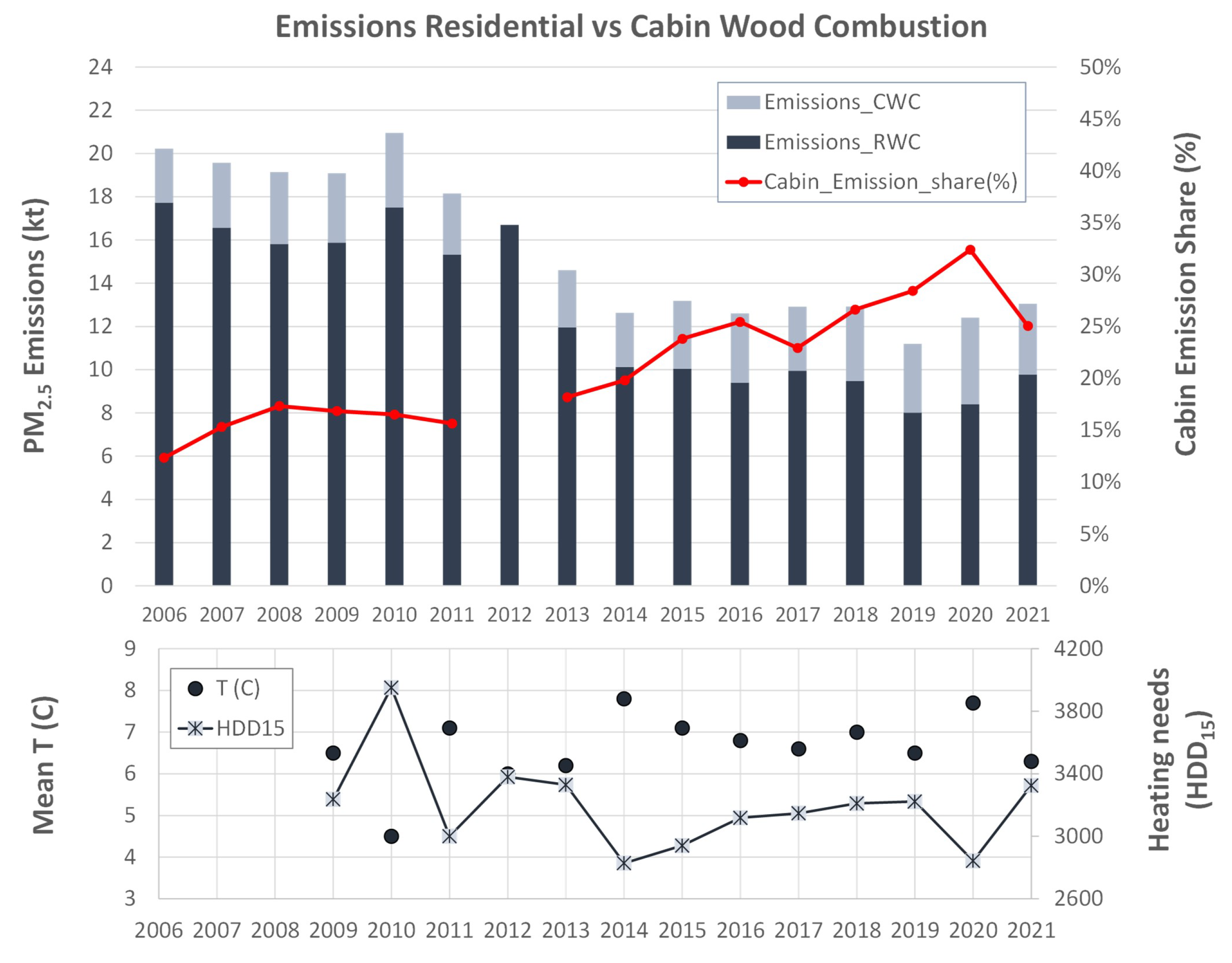The sampling error is estimated to be 3% on the national scale, and there are separate questions for other properties (for details, see [17]). As there is no other available source of wood consumption for heating in residences or cabins at national scale, this data source represents the main input data to estimate wood combustion for heating. However, the annual total number of heating degree days (HDD) was found to explain ($\mathrm{r}2=0.8$) the inter-annual variations in consumption between 2005 and 2018, indicating that wintertime temperatures can also be a good indicator for RWC [17].

Wood consumption for residential and cabin heating are available on a yearly basis and split into consumption in old stoves (manufactured before 1998), new stoves (manufactured after 1998) and open fireplaces. While for residential heating, wood combustion per technology is provided at the county level, in the case of cabin heating, the wood consumption is reported for 5 regions, where each region contains several counties, and the split in technology is only available at national level (for more detail see Section 2.2).

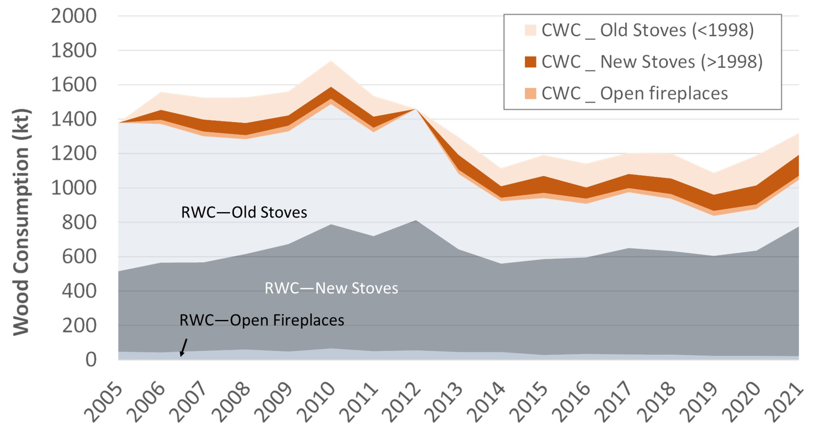
The trend of wood consumption for residential and cabin heating have been analyzed for the period between 2005 and 2021 (Figure 2), and a declining trend in RWC is found from 2005 to 2019. This decline is related to more energy efficient buildings, lower shares of wood as a heating source and more efficient stoves, despite more and larger residential buildings. In 2020, the decline was interrupted when, even experiencing the warmest winter season, COVID-19 and the imposed lockdowns affected human activity and increased time at residences, which is related to higher residential wood burning activity. The increase in 2021 regarding preceding years may resemble the still higher activity at residences due to COVID-19 (e.g., home office), in addition to the increase in electricity prices from September 2021. Conversely to RWC, wood consumption in cabins experiences few changes over time or even a slight increase from 2014 (Figure 2).

2.2. Cabin Stoves

There are estimated 820,000 stoves in the roughly 450,000 cabins in Norway according to “Norsk Varme”, an association of wood burning stove producers. Due to the type of input data available, the stove technology is linked to the wood consumption as it is reported per technology class installation. In the case of CWC, we use the national split of wood consumption per technology for all regions [14]. For instance, national wood consumption in cabins in 2019 was registered to be 51% old stoves, 37% new stoves and 12% open fireplaces [14]. Wood consumption per technology may have geographical differences, however, additional available data support this assumption. The MetVed emission model includes data from the Fire and Rescue agencies, which are responsible for inspecting and assessing all firing installations. This data-set contains the complete information from around 100 municipalities, covering 1 million of the 2.5 million dwellings in Norway. Within those buildings classified as cabins, 26% of the wood installations are classified as new stoves, 61% are old stoves, and 13% are open fireplaces. These data support the assumption concerning the wood consumption split, and the data-set does not show strong regional differences. The Fire and Rescue agencies data-set also confirms the number of wood stoves in cabins in Norway (i.e., 820,000 stoves), where, even for coastal cabins, over 1.5 installations per cabin are estimated.

2.3. Emission Factors

The emissions factors (EFs) used in MetVed are the same as those used by Norway for the reporting of emissions to the CLRTAP [19], and are used to calculate emissions from both RWC and CWC. The EFs per technology are obtained via particle sampling in a dilution tunnel, mimicking the dilution and cooling effects after the smoke exits the chimney, and accounting for the formed condensable matter [6]. These EFs also take into account that emissions depend on how the stove is operated. Hereby, EFs are provided for part-load and nominal-load operating conditions for each stove technology. Our study considers 65% part-load and 35% nominal-load split for old stoves, and 70% part-load and 30% nominal-load operating conditions for new stoves [6]. The EFs for PM${}_{2.5}$ are 7.85, 20.86 and 16.40 g kg${}^{-1}$ of dried wood, for new stoves, old stoves and open fireplaces, respectively. The EF for $\mathrm{P}{\mathrm{M}}_{2.5}$ emissions from RWC in Norway is steadily going down due to the renewal of stoves [20]. However, the reduction is slower for CWC (for more detail, see Section 3).

2.4. Location and Classification of Cabins

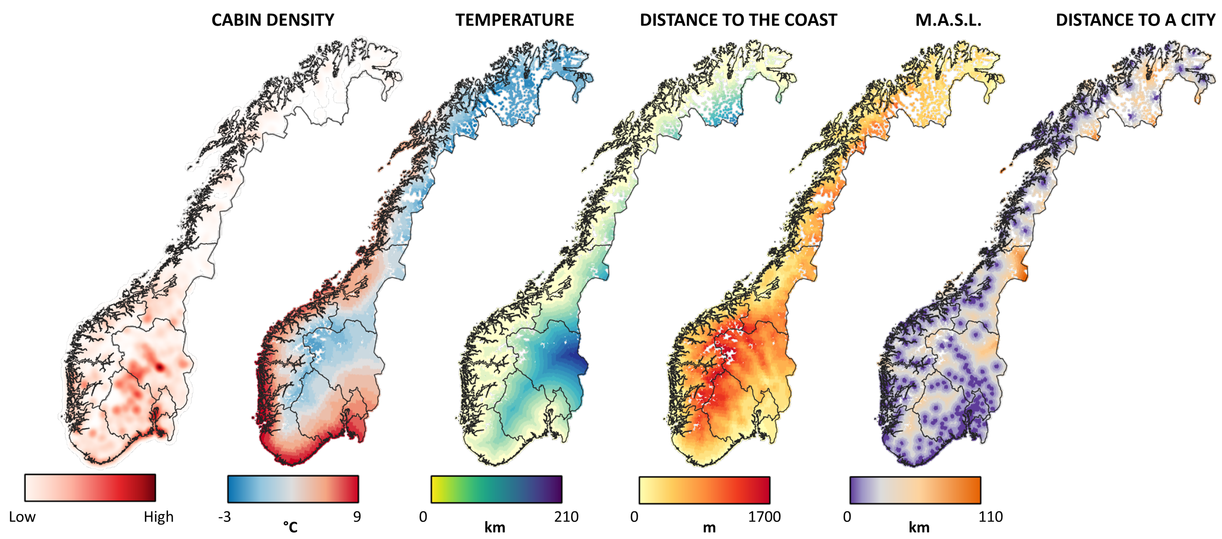
The number of all the buildings in Norway, including residential and cabins, are openly available from Statistics Norway on a 250, 1000 and 2000 m grid since 2008 to 2021. This information represents the basis for the distribution of emissions. Cabins are geographically distributed to serve several purposes, and the highest density of cabins is along the coast (Figure 3). Coastal leisure activities are for the most part limited to summer, whereas cabins in the mountains are considered to be more of a full year destination. In order to estimate emissions, the consumption of wood needs to be determined by the heating need and presence of other heating sources. The heating need depends on the buildings heat efficiency and the difference between ambient outdoor temperature and the desired indoor temperature, which is largely determined by the season the cabin is used.

To differentiate cabin types, we made a set of parameters to classify each cabin (grid) as either “alpine” or “coastal”, as the occupancy of these cabins will have very different seasonal profiles (see Section 2.5) and presumably different qualities. This method represents an advancement regarding other studies in the literature. For instance, Plejdrup et al. [18] discriminate between residential dwellings and holiday houses in their RWC emission model for Denmark by applying different weighting factors. However, they do not discriminate between a holiday usage in summer or winter as it is necessary in the case of Norway.

We assigned different attributes to each cabin grid in the emission model to classify type/usage of cabins. The distribution of such properties or attributes and the cabin density are shown in Figure 3. The attributes are (i) the distance to the coastline; (ii) the distance to a city center; (iii) the altitude of the cabin grid; and (iv) the annual mean temperature of the grid where the cabin is located. The distances to the coast and to the nearest urban center are calculated for each grid as the shortest straight line to the coastline and to the nearest urban center centroid, respectively (Figure 3). These distances are static parameters for the time series as the locations, e.g., city centers, barely changes on our timescale. The mean annual temperature of the cabin grid (Figure 3) is taken from ECMWF (the European Centre for Medium-Range Weather Forecasts) reanalysis fields at a 0.1° × 0.1° resolution. This resolution (approximately 10 × 6 km) is probably too coarse to pick up local effects, such as fjords or valleys; still, it gives an overall description of the climatic features of each cabin grid. The cabin grid surface elevation to establish the cabin altitude relies on ECMWF data, specifically on the surface average geopotential (m s${}^{-2}$) divided by the gravitational constant. The above mention properties, i.e., altitude (m) and temperature (°C), are bilinearly re-gridded to the cabin grid and added to the cabin properties. Together, these cabin properties provide the necessary additional information to classify each cabin as alpine or coastal.

In order to classify the cabins in the two categories, different thresholds were evaluated by visual inspection and the comparison of the locations of cabins classified as alpines or coastal. Based on this analysis, when a cabin is located above 400 m.a.s.l, more than 15 km from the coast, or the grid annual average temperature is below 2 °C, this cabin is classified as alpine. The latter criteria are only relevant in Northern Norway.

2.5. Cabin Occupancy

In addition to having a stove installed, heating by wood requires the presence of people to start and feed the fire. Therefore, the residence time or occupancy of cabins needs to be determined to temporally resolve wood consumption in cabins. Even though cabins are mainly used for leisure activities or holidays, information on the time spent in privately owned accommodations is not reported in the way international travel and stays in commercial institutions are. It is, therefore, much less data to base calculations on, and a parametrization was developed to determine cabin usage.

Based on previous analysis of national travel surveys and additional documentations (e.g., 36% of Norwegians have access to a cabin), people who owned a cabin spend on average 30 nights per year distributed over 12.5 trips [21]. Other investigations have also shown that longer time is spent on the cabin if the cabin is closer to the place of residence. The primary assumption for our parametrization is that the relative amount of people in a specific area generate local traffic. This is supported by the fact that over 90% of people select the car as a transport mode for visiting the cabins. An increase in traffic counts was previously suggested as a data source to determine the amount of cabin visits [22,23]. Therefore, an ancillary data source that represents when people are at cabins is the additional road traffic created by them.

The Norwegian Public Roads Administration (NPRA) database is available through an API of approximately 12,000 automatic traffic loops. The NRPA has national responsibilities and cover national roads, whereas regional and local roads are administrated by local authorities. As a consequence, most of the counting points are on main roads. To obtain a clear signal of the traffic activity associated with cabin visits, two automatic traffic counting stations were selected based on their locations. The priority was given to stations that represent areas with a high number of cabins, and additionally, that the roads where the counting is located do not have a large amount of transitional traffic. Few suited traffic stations were found for the analysis, and the two selected stations are in Hvaler and Trysil. Both traffic counting stations share that they do not have much transitional traffic and both have a large cabins to residential buildings ratio. Trysil is located at Kirkebrua in the mountains, has a skiing resort and is the municipality in Norway with the second highest number of cabins [14] (i.e., 6530 cabins). Hvaler station is located at the Bukkholmen bridge, which connects the mainland with an archipelago in south east Norway resulting on a dead end road, and is in the top ten municipalities concerning number of cabins (i.e., 4310 cabins), which are commonly used in summer.

Hourly two-directional traffic data of short vehicles (<5.6 m) in 2019 was used in this analysis. For each weekday, the daily “excess traffic” was calculated as the traffic volume above the 25th percentile for each weekday (Figure 4A, for coastal cabin and B for alpine cabin), and thereafter combined with the Norwegian Calendar that defines holidays. This gives the increase in the traffic volume for each holiday. Days were categorized as full or half holiday. Hereby, days with a holidays before and after were set as full holidays, whereas the opposite for half holidays. In that way, and for weekends, Saturdays are defined as full holidays, whereas Fridays and Sundays are half holidays. This is due to the fact that Fridays and Sundays are traveling days involving traffic increases. For longer holidays, the traveling day is the day before the holiday and the last day of holiday. Christmas Eve and New Year’s Eve were treated as full holidays for every year.

An excess of traffic was defined for the traffic counting data-set from NPRA for 2019. The excess traffic was defined as traffic above the 25 percentile daily traffic for each individual counting point. The excess traffic was then used to define days with increased traffic. When compared to the holiday calendar, the two counting points showed on average 5.4 times more excess traffic relative to workdays. The excess traffic was then used to set the usage ratio between holidays and working days for each type of cabins. On any given day, the cabin usage was assumed proportional to the increase in excess traffic. To make this approach applicable to any year, the usage rate for each day of the year was associated with the type of day it was, where type was defined by moving and stationary holidays, and weekdays. The traffic variability is combined with the number of nights on average spent in cabins to obtain an occupancy fraction throughout the year. The result is a parameterized week number, weekday and holiday weight used in the model as a .csv file. The moving holidays summer, autumn and winter are defined by their week-number, whereas a function to calculate Easter day is used to place the Easter holiday. Figure 4 shows the fit of data to 2019, where the usage rates of the two different cabin areas (C and D, coastal and alpine cabin, respectively, Figure 4). The coastal cabins (Hvaler) show a much clearer seasonal pattern than the alpine cabin (Trysil). From November to March, the usage of coastal cabins is negligible, with the first peak occurring in Easter. The highest usage of coastal cabins is in July and summer weekends, with a very small peak in Autumn school holidays. The usage of alpine cabins is more evenly distributed in weekends and holidays throughout the year, with the most marked peaks around Winter, Easter, Autumn holiday weeks and Christmas/New Year.

2.6. Cabin Heating Needs

In Norway, almost all cabins have a stove or fireplace, and the need to heat the cabin is linked to the outdoor temperature. In the case of cabins, wood consumption for heating depends on the occupancy and the season when the cabin is used. This is for the most part relevant for coastal cabins, as they have shown a strong seasonality in occupancy (Figure 4). A common method to describe the heating needs is the heating degree day (HDD), which in our study is also connected to annual average temperature. The HDD for both coastal and alpine cabins is only estimated for the period when the cabins are occupied (Figure 4). The difference in total HDD in 2019 between both locations was estimated to be a factor of 2, i.e., Hvaler, 2600 HDD${}_{15}$; Trysil 5300 HDD${}_{15}$, considering a threshold for using wood for heating of 15 °C as it was considered for residential heating emissions [17]. Considering that the difference in annual average temperature between Hvaler and Trysil in 2019 was estimated to be about 3.2, the relationship between annual temperature and HDD was establish to be at 0.62 HDD °C${}^{-1}$. This relationship, and ignoring other influencing factors, predicts a difference in the heating demand of 2 based on the annual average temperature at cabin locations defined as alpine and coastal. This difference is in agreement with the relationship between the two locations of the traffic counting station, i.e., Hvaler and Trysil, and verifies the representativeness of these two locations. Taking into account the difference in cabin usage between alpine and coastal cabins, this factor increases to 6.4 (2019) as the usage of alpine cabins is enlarged in colder periods, and therefore during heating season, in contrast to the usage of coastal cabins.

Alone, the grid average temperature in a region is not very predictive of the wood consumption in an average cabin. As total wood consumed is prescribed to a region, normalized temperature was used for each separate region. A benefit of this is that the normalization reduces potential regional border effects. A weighting factor of 0.8 was applied to temperature to account for the assumed lower heating need of a cabin in colder area. The reasoning behind this is that we assume cabins are somewhat adapted to their location, and that cabins in colder regions will have better isolation.

2.7. Emissions from Wood Combustion in Cabins

In order to determine the spatial and temporal distribution of emissions from CWC, cabin occupancy and a developed wood burning potential from cabins were used as distribution key. The wood burning potential of a cabin is determined in relation to the other cabins of each region, and then used to spatially allocate wood consumption in a geographical region. The wood burning potential ($WP$) is calculated at the grid level (g) based on the number buildings classified as cabins in the grid (C), the cabin type weight ($C{T}_w$) and HDD weight ($HD{D}_w$) as:

$$W{P}_g=C\times C{T}_w\times HD{D}_w$$

(1)

where the $HD{D}_w$ is defined to reduce the effects temperature has on consumption by multiplying the regional temperature z-score by 0.2. In order to obtain wood consumption at the grid level, the normalized wood potential is multiplied with the total wood consumption per technology in the region where the grid is located and the local EFs per technology to arrive at annual emissions from CWC.

3. Results

3.1. Residential Wood Combustion Emissions Trends

Figure 5 shows total PM${}_{2.5}$ emissions from residential heating, including both RWC and CWC since 2006 to 2021, along with mean temperature and total heating needs. The mean temperature represents the average overall dwellings, where temperature is given as the value from the geographically closest measurement station with valid observations. The total heating need is estimated as the total number of HDD${}_{15}$ averaged over all dwellings in Norway.

While total emissions show a clear downwards trend up to 2019, the trend is reversed in the last two years. Whereas, emissions from RWC have been reduced (from 2006 to 2019), CWC emissions has been kept constant or even slightly increased (Figure 5). This opposite trend implies that cabin emissions shares to total emissions increase overtime from around 12% in 2006 up to 25–35% in the last years.

The reduction in emissions from residential heating has been mainly driven by a reduced trend in the consumption of wood, but also by a shift to newer and cleaner stoves. The stove replacement to cleaner installations has mainly been observed in residential buildings, whereas this process is slower in cabins. The reason behind may be linked to regulation of RWC emissions, in which policy instruments have a stronger focus on urban residential areas [5]. The technology replacement mainly acts to reduce EFs, i.e., the emissions per consumed dry wood, but also newer stoves are reported to be more efficient, producing more heat from the same amount of wood. The long-term decline in consumption has previously been studied [17], and influencing factors were found to be; (i) increased share of other heating technologies, especially heat pumps and district heating; (ii) more energy efficient buildings; and (iii) lower winter outdoor temperature reducing the demand for heating.

While 2020 was the warmest year on record, and the total heating need dropped from 2019 by 12% (Figure 5), emissions increased. There are diverse reason for the reversal of the trend, which shows increased emissions over to 2021. There is a probable influence on wood burning emissions by the COVID-19 pandemic. The two most prominent COVID effects are: (i) time spent at home increased, especially during lockdowns, and (ii) travel restrictions affecting the time spent in Norwegian cabins. Both of these changes in activity act to a net increase in consumption and subsequently emissions. Similarly, increased usage of cabins increases the expected consumption there. The latter, in addition, has the overall effect that it acts to increase the average age of stoves, and thus the emission factor, as cabins have significantly older stoves than those in residencies. Our results are in line with reported changes in emissions due to the COVID-19 pandemic, where a slight increase in $\mathrm{P}{\mathrm{M}}_{2.5}$ emissions from residential wood combustion at European level was reported [24]. Opposite to 2020, 2021 was the coldest year since 2013, and thus the total heating need increased from the previous year (Figure 5), driving wood consumption up. In addition, still COVID restrictions and higher flexibility of home office can possibly explain the increase in wood burning emissions. Moreover, since September 2021, a marked increase in electricity prices in Norway occurred, which resulted in record sales of wood.

3.2. Spatial and Temporal Distribution of Emissions

Heating activity occurs differently in space and time in residences and cabins, based on where cabins and residences are located and when they are vacant. To highlight the difference, Figure 6 shows emissions produced for residential (left) and cabin (right) PM${}_{2.5}$ wood combustion for heating as heat maps. The largest hotspot of emissions from RWC occurs in and around the main cities in Norway, and most pronounced around Oslo. Hotspots of CWC are found in central Norway, mostly in areas with cabin agglomerations around ski resorts. While much of the cabins are along the coast (Figure 3), these areas are not identified as areas of high emissions. This is a result of the proxies applied in our study to account for differences in occupancy between alpine and coastal cabins, which gives the time spent in coastal cabins, mainly summer, a very low heating demand compared to alpine cabins. This also results in a different temporal distribution of emissions between residencies, alpine and and coastal cabins. Occupancy of cabins, and consequently use of wood stoves, varies strongly throughout the year and week. Figure 7 shows the time variation of emissions for RWC (Residential) and CWC (coastal and alpine cabins). RWC emissions occurs mainly during the winter months, at weekends and during the evenings. The monthly variation shows the “U-shape” characteristic of residential heating with a minimum during summer. While the same heating demand influences time variation of emissions from CWC, their emissions follow more strongly their occupancy during the year. Coastal cabins have the highest peak in spring due to the combination of occupancy and $HDD$. There is also an emission peak in July, when coastal cabin has their peak occupancy, mainly evident in colder parts of the country. Alpine cabins have their highest activity in the holidays in winter and spring, which results on emission peaks due to the substantial heating demand in this period. Whereas Christmas and Easter is the same all over Norway, the week of autumn and winter holiday varies across the country, and the national emissions peaks are therefore less pronounced. Furthermore, Easter day, which determines the holidays of Easter, can make the holiday fall in either March or April from year to year.

4. Discussion

The use of common proxies in the development of regional emissions from heating, which are more representative of residential emissions, involve errors with consequences for modeling the transport and deposition of air pollutants, and assessing local and regional air quality plan. Our study shows, with the example of Norway, the complexity of distributing emissions from residential heating at high spatial and temporal resolutions. Our study considers a factor that has not received significant attention in the literature, which is the distinction of primary and secondary homes. In Norway, about 20–30% of the residential wood combustion takes place in second homes or cabins (CWC), and considering that occupancy has been reported to be around 30 days per year, involves that CWC is 13 times more intense than wood combustion in permanent residential addresses (RWC). Moreover, as cabins can be classified as coastal and alpine, mainly used in summer and winter, respectively, wood burning will be even more intense due to the seasonal differences in heating needs.

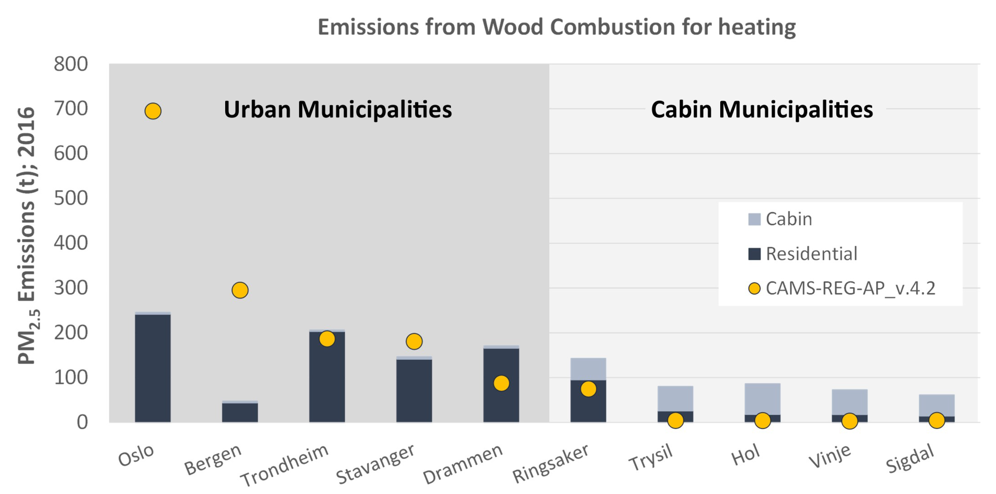
Emissions obtained in our study have been compared for specific municipalities with emissions from residential heating (NRF Sector: Residential Stationary) available through Copernicus Atmosphere Monitoring Services (CAMs [25]). For our comparison, the most populated urban municipalities were selected, i.e., Oslo, Bergen, Thondheim, Stavanger and Drammen, representing around 24% of Norway’s population. Moreover, the five municipalities with the highest density of cabins were chosen, i.e., Ringsaker, Trysil, Hol, Vinje and Sigdal, representing around 7% of the cabin stock in Norway. Figure 8 shows the comparison of emissions produced in our study for the mentioned municipalities with the same sector from CAMS-REG-AP [7]. While our emissions for the two biggest municipalities (Oslo and Bergen) are much lower than those produced by CAMS-REG-AP, the proxies behind CAMS-REG-AP do not allocate emissions in most of the cabins municipalities showing a clear correlation with population. The reason is that the regional emission inventory distribute emissions from residential stationary as exclusively from residences, and does not consider a different proxies for the use of wood consumption for heating in cabins, which represents a large part of the emissions reported as residential stationary. As a consequence, the gradient in heating emissions from rural to urban is much larger in CAMS emissions than in our study. Considering that residential emissions produced in our study have been extensively validated for Norwegian cities by comparing modeling results with observations [17,26,27], the gradient obtained in our study better represents local emissions in rural and urban areas than those provided by CAMs.

Our study shows the relevance of discriminating between primary and secondary homes in Norway to avoid an overallocation of emissions in urban areas and underestimation in densely populated cabins areas. This aspect can be relevant for other countries, where having second homes is very extended, such as other Nordic countries, and partly explained by wealth and availability of space (e.g., [28]). For instance, in Finland, with a similar population to Norway, there are approximately 500,000 recreational houses, where wood is used for heating [29]. In Denmark, the total wood consumption in holiday houses, even though assumed to be mostly used in summer, is approximately half of the consumption in permanent residences [18]. In the Alpine Region, second homes are estimated to be around 1,850,000, around 25% of the housing stock, and are expected to grow in the future [30]. Taking into account that the occupancy of holiday houses is much lower than that in primary houses, wood combustion for heating represents an intensive activity in short periods of time. In mountain areas for instance, and those affected by intense tourism activities, it represents the largest energy source for heating, the emissions of which, intensified by temperature inversions and topography, result in high pollution episodes and additional environmental impacts (e.g., [31,32,33]). Moreover, wood burning is one of the largest sources of black carbon [34], and its deposition in snow, along with dust, has been estimated to be responsible for advanced snowmelt of around 17 days on average in mountain areas such as the Alps and Pyrenees [35], with subsequent impacts on mountain ecosystems, water resources and society.

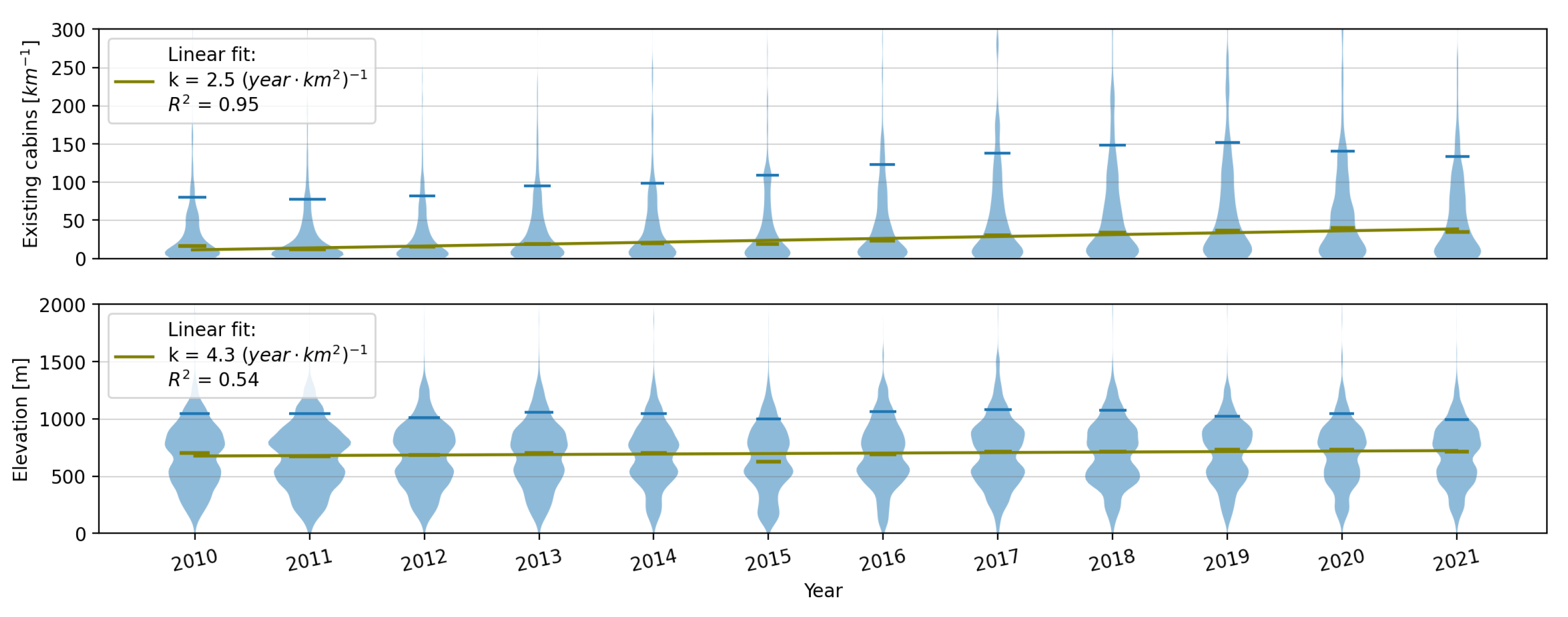
Wood burning for heating of secondary homes or cabins is an aspect that also needs to be considered for future assessments of cabin development plans in rural areas. We have analyzed webcrawled data from the state market portal in Norway ([36]) in combination with the annual gridded building data, and the results indicate that new cabins are mostly built in areas with existing cabins, creating cabin settlements. Moreover, the share of newly built alpine cabins has increased over time from 60% in 2010 to 70% in 2021. Figure 9 shows the alpine cabin distribution based on the building year (x-axis) and the location where they are built based on the number of existing cabins (km${}^{-2}$; y-axis), along with the median (green line) and the 90th percentile (blue line). While in 2010, the median number of existing cabins per square kilometre for newly built alpine cabins was estimated to be 12 km${}^{-2}$, it increased to 40 km${}^{-2}$ by 2021, with a trend of 2.5 per year (Figure 9). Moreover, from 2015 to 2021, 10% of the new cabins were built in areas where there were already 100 or more existing alpine cabins. New cabins are being built at higher elevations, with median rising from 630 m in 2010 to 730 m in 2021. The new cabin development is, therefore, resulting in the creation of cabin settlements and higher densification at high altitude. The strong periodicity in emissions, following the holiday calendar, further suggests this episode of extreme emission intensity. This can also be exacerbated in 2022 due to the increase in electricity prices. Hereby, subsides are in place in Norway to support the high electricity prices that started in September 2021, and have continued upwards over 2022. However, the subsidies only apply to residential buildings, and second homes are excluded, therefore the incentives are to rely on alternative heating sources, mainly wood. Moreover, land use changes associated with cabin development has been highlighted along with the need for stricter land use and building regulation [37]. Second homes, such as cabins, and the tourism associated with are increasing worldwide [38,39]. Therefore, emissions from CWC may become an increasing concern, which needs to be capture in regional emission inventories to assess potential environmental implications, and avoid the allocation of such emissions in urban areas.

5. Conclusions

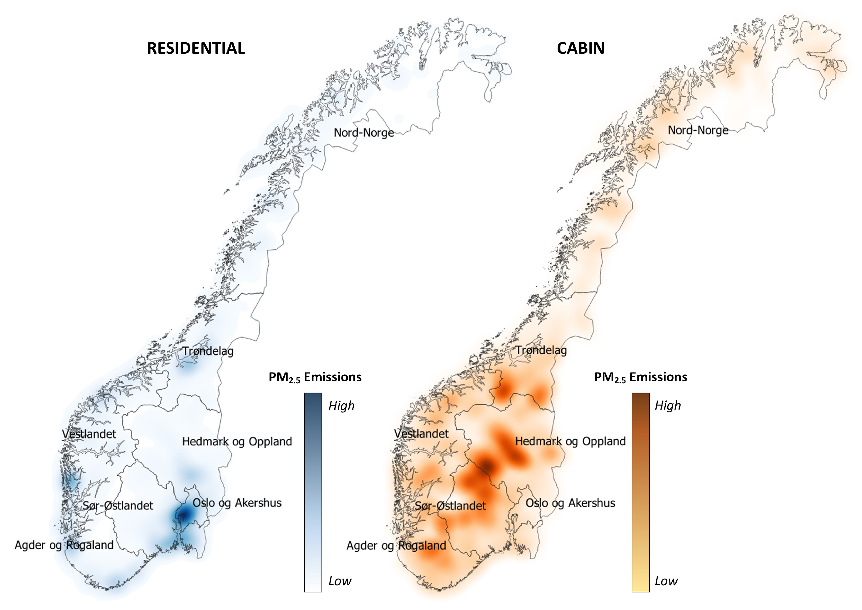
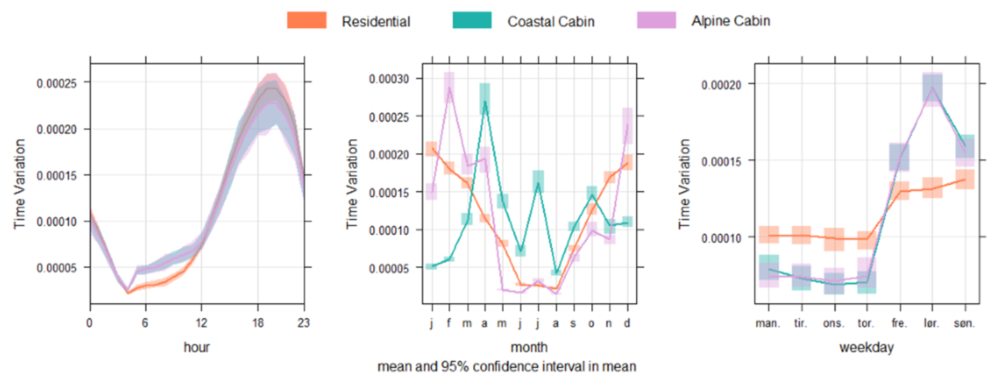
High-resolution emissions are essential for air quality assessment and management. Our study takes into account an aspect beyond the spatial and temporal distribution of emissions, which is the use of wood burning for heating in secondary homes or cabins. Norway, with a population of around 5.5 million, has ca. 450,000 cabins, and even though 2% of the time is estimated to be spent at cabins, around 20% of the wood consumed and 30% of the emissions for heating occurs there. Our study has first presented a novel method to estimate emissions from cabins at high resolution based on the analysis of traffic data and, thereafter, determining cabin occupancy for coastal and alpine cabins. By combining wood burning emissions in permanent residences (RWC) and cabins (CWC), our results show that while emissions from RWC are distributed mainly around cities and townships, emissions from CWC are more spread in the geography with large hotspots in mountain areas with high densities of cabins, even though the highest cabin density is along the coast. When analyzing the temporal variation of emissions, RWC emissions show a characteristic “U-Shape” with high emissions in winter and low or zero emissions in summer, whereas coastal cabins show high activity in Easter week, July and Autumn holidays, and alpine cabins show peak emissions in winter holidays and Christmas holidays. The spatial and temporal analysis indicates that a temporally “cabin population” can in areas be orders of magnitude larger than the registered population, and emissions are specially intense in holidays.

The emissions estimated in our study have been compared with a regional emission inventory commonly used to model transport and deposition of air pollutants (i.e., CAMS-REG-AP). The comparison shows large discrepancies between municipalities that contain the biggest cities, and municipalities with the highest density of cabins. While the regional inventory does not allocate emissions in the cabin municipalities, much larger emissions are allocated in urban municipalities than those obtained in our study. The CAMS-REG-AP spatial distribution results in a stronger gradient in emissions from more rural to urban areas than that obtained in our study. This discrepancy can occur in other countries or regions also characterized by intense wood burning activity for heating, and a large share of second homes. Some of these regions are mountain areas, where additional temperature inversions, topography and the fact that heating is the prominent local emission sources, will involve local pollution episodes, and for instance the deposition of black carbon with subsequent snowmelting effects.

Cabins are an increasingly important consumer of energy, and wood is the primary heating source, which is not expected to change in the future. Our study shows an increasing trend in the cabin stock in Norway along with a higher densification in mountain areas. The nexus between cabin development, energy use and emissions needs to be considered in future assessments and in the context of rural development and building regulation in areas such as mountain areas.