A Study on the Development of a Novel ESS Simulation Model for Transmission-Level Power-System Analysis

Abstract

Thanks to technological advances, the number of large-scale ESS applications is increasing in power systems. Therefore, the need for an ESS model to analyze the effect through simulation has also increased. In this study, an ESS analysis model was developed for transmission-level power-system analysis. The developed model has a relatively uncomplicated configuration compared to the previous model. The ESS model was developed in a form that can be exploited in the PSS^®E, commercial power-system analysis program. The programming language FORTRAN was used for model development. A detailed process and necessary data for the model development are described. The operation of the developed ESS model was verified through simulation using two test systems. The results of this study can be used for power-system analysis and as reference material for model development.

1. Introduction

Power-balance and power-quality problems are caused by the difference between power supply and demand. An energy storage system (ESS) can be used to reduce the difference between the supply and demand of electricity. Moreover, utilizing ESS, it is feasible to enhance power quality and respond to a power supply and demand crisis. The number of ESS applications in the power industry is increasing. ESS can play a role in managing peak load, stabilizing the output of renewable energy sources [1] and regulating system frequency. Various demonstrations of ESS in connection with renewable energy sources are in progress through international efforts to reduce greenhouse-gas emissions. ESS is considered a countermeasure for supply shortage due to aging power facilities. The detailed ESS applications in the power system are described in Section 2.1.

Currently, the ESS industry mainly focuses on batteries of a scale used for electric vehicles. However, the utilization of large-capacity ESS in the power system is also increasing [2]. Batteries [3,4], flywheel energy storage [5,6], supercapacitors [7,8,9], compressed air energy storage (CAES) [10,11] and superconducting magnetic energy storage (SMES) [12] are the most popular items. In addition, various studies on hybrid types combining two or more ESSs are being conducted [13,14,15,16,17,18].

The installation of ESS affects the power quality of nearby systems [19,20,21,22]. Therefore, an analysis procedure that can investigate the impact before installation is required for a system’s stability. Depending on the capacity of the ESS, the effect on the power system is different, and the input of a large-capacity ESS may require a transmission-level system analysis [4]. Therefore, an ESS analysis model has to include the proper characteristics for the simulation [23]. The “CBEST” model is one of the ESS analysis models in commercial analysis programs. In transmission-level analysis, the “CBEST” model is widely used because its configuration is simple and easy-to-use. However, this model has limitations because it reflects only the fundamental characteristics of ESS. The characteristics of the already developed and popularly used ESS analysis model, including “CBEST”, are summarized in Section 2.2.

In this study, an ESS analysis model was developed for transmission-level power-system analysis. The developed model is not simply a test model for research but is usable in PSS^®E, a commercial power-system analysis program. In addition, it is not complicated because it has only essential parts for the simulation.

PSS^®E uses the programming language FORTRAN for modeling. The modeling process and detailed configuration of the developed model was described in this study. Two test systems were used to validate the model. First, some simulations were performed to verify the developed model in the simple test system. Second, in order to verify that the developed model operates properly in a general system, a simulation was performed in the IEEE 14-bus power system, and the result was confirmed.

The rest of the paper is organized as follows: In Section 2, this work briefly explains the background of this study, such as ESS application in a power system or ESS models in transmission-level analysis. In addition, this study describes the user modeling overview in PSS^®E. In Section 3, the developed ESS analysis model is presented. The description of the overall model and each part are described in detail. In Section 4, the developed ESS model is verified by simulation. Finally, the conclusion is drawn in Section 5.

2. Background

2.1. ESS Applications in a Power System

ESS is able to play various roles in a power system. As a technology to increase the balance of power supply and demand, price competitiveness, and energy efficiency, it secures the operating reserve to effectively respond to peak load and blackout. This paper targets a relatively large ESS analysis model, some utility-scale-level applications are summarized in this section [24,25,26,27].

• Peak shaving: The most well-known feature is storing energy in low-demand situations for high-demand use. This function is known as peak shaving/load shifting/load leveling, and is one of the essential functions of ESS.
• Reduction in congestion: Congestion on the line can be reduced using ESS. Proper ESS installation can avoid network expansion, which incurs high costs.
• Frequency regulation (FR): If an imbalance occurs in the power supply and demand, the power quality cannot be maintained due to frequency fluctuation. Frequency fluctuation appears throughout the whole power system. Using ESS for FR can be helpful to maintain the rated frequency [28].
• Voltage regulation: Voltage regulation is closely related to the reactive power supply and has a local characteristic. An ESS installed in an appropriate location helps with voltage regulation: to maintain the voltage within normal operating ranges [29].
• Operation reserve: ESS can provide a spinning reserve to the power system.
• Renewable energy utilization: Renewable energy sources such as photovoltaics (PV) or wind power put a burden on the power system’s operation due to its high output variability. If ESS is used together with renewables, the output can be stable, which helps increase the amount of renewable installation and power system stabilization [30].

2.2. ESS Analysis Models in Transmission Level

2.2.1. “CBEST” Model

When performing system analysis, an analysis model of battery energy storage systems (BESS) is needed. The “CBEST” model is one of the ESS analysis models for BESS simulation, which is frequently used in power-system simulation. In commercial programs such as PSS^®E or PowerWorld simulator, the “CBEST” is in the model library [31,32]. This model is developed by EPRI and has an uncomplicated structure, so it is often used for power-system analysis. Each control of active and reactive power is possible using the “CBEST” model. This model shows BESS characteristics using appropriate limits. Since it supplies power to the system directly, it is classified as a generator model in the model library.

When the BESS capacity is small or other factors are relatively dominant in active power supply, its effect is limited in a power-system simulation. In this case, there is no problem in simulating with the basic control characteristics and the input/output characteristics of active and reactive power. However, there are some limitations in the “CBEST” model when performing a simulation in which the characteristics of BESS must be shown in detail. For example, it may be difficult to use the “CBEST” when generator-level control is required for active and reactive power or for parts that require control related to the state of charge (SOC).

2.2.2. ESS Models in Power-System Analysis

The ESS analysis model has been developed from the development of a model which converts, for example, wind power or solar power to the form of the ESS generic model currently used. The Western Electricity Coordinating Council (WECC) has released a library for power-system analysis, and related models are also provided in the PSS^®E program.

Table 1. ESS analysis model comparison.

Type	PSS®E	WECC	Note
Control	REECA1	REEC_A	Renewable energy electrical control model
	REECB1	REEC_B	Renewable-energy electrical control model for large PV
	REECCU1	REEC_C	Renewable-energy electrical control model for ESS
Machine	REGCA1	REGC_A	Machine model (generator/ converter)

summarizes the models related to renewables and ESS.

In Table 1, WECC models and PSS^®E models are described. As the PSS^®E program accepts the model released by WECC, even though some changes suit the program’s characteristics, most of them show similar forms. The ESS analysis model currently used for power-system analysis consists of electrical control and machine models. The schematic diagram of those models basis is shown in Figure 1.

The control model receives the feedback signal of the terminal voltage. It performs the necessary control operation and then transmits current commands to the generator model. Most of the various control tasks of ESS are carried out inside the control model, and the generated current command is related to controlling active and reactive power. After receiving a signal from the control model in the machine model, a current is generated and injected into the power-system network. Even though there are some differences between the ESS model and the renewable model in detail, the type-four wind generator and PV analysis models also have a similar configuration.

2.2.3. User Modeling in PSS^®E [33,34]

PSS^®E is a widely used program worldwide, and it is able to analyze the general area of the power system. The program provides a wide range of functions, such as power flow, dynamics, short circuit, contingency analysis, optimal power flow, voltage stability, and transient-stability simulation. As mentioned above, this paper aims to develop a user model which can be used for dynamic simulation in PSS^®E.

The dynamic simulation aims to simulate a transient response in a designated time frame when an accident occurs. Therefore, each power-system’s facilities have to be expressed as an analysis model which accurately shows its transient section characteristics. PSS^®E has various model libraries, so users can simulate the transient state by setting parameters after selecting a model. However, even though there are various types of built-in models, in some cases, there may be cases where there is no analysis model of the facility required for analysis. In preparation for such a case, PSS^®E provides a model writing technique so that users can directly create a model of necessary facilities. The model developed is named the user-defined model (UDM).

For a user to implement a specific facility with a UDM, it is necessary to understand the program structure. In Figure 2, each element’s characteristics are schematically expressed when the analysis is performed by inserting the user model in PSS^®E. Data input/output and most of the analysis tasks are performed in the main skeleton part. When the user uses UDM, the simulation proceeds by exchanging necessary information with the main skeleton part and working-arrays part. The working-array part is responsible for storing data during the dynamic simulation and uses the following four memory arrays.

• CON: contains constants (not varied during the simulation).
• STATE: contains state variables (determined by differential equations).
• VAR: contains algebraic variables.
• ICON: contains integer quantities (specified by logic).

Figure 2. Schematic diagram of PSS^®E simulation.

Figure 2. Schematic diagram of PSS^®E simulation.

3. ESS Model Development

3.1. Model Overview

As mentioned earlier, most analysis models for power-system simulations are divided into control and generator parts. However, this study aims to construct a simple model which contains only essential functions for transmission-level analysis. For this reason, the ESS analysis model was developed as a single generator model, and the schematic form is shown in Figure 3.

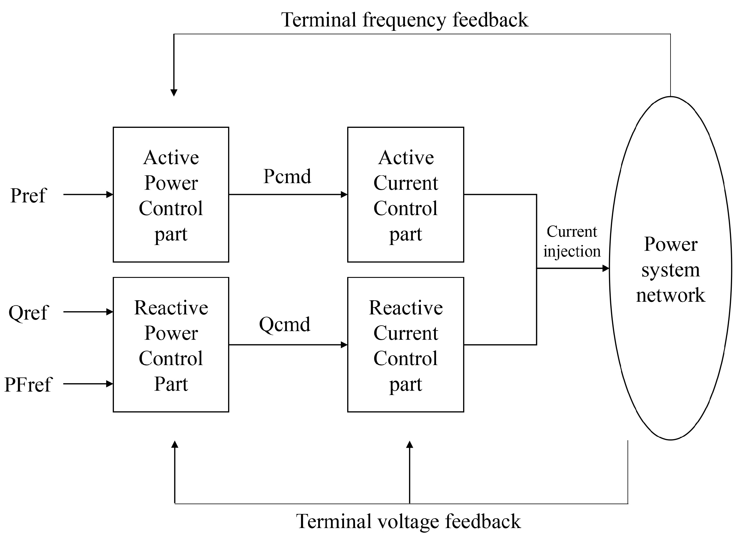
Figure 3 shows a schematic diagram of the developed ESS analysis model. In order to inject electricity into the power system in the PSS^®E program, a form of a current injection model is required. Therefore, the developed ESS model was also implemented as a current injection model. Considering the current ESS characteristics, the active/reactive power can be controlled independently, so each part was developed separately. Figure 3 shows that the control part generates two control signals by receiving active/reactive power reference, power-factor reference, terminal voltage, and system frequency as inputs. In the control signal generation process, various processes for control are performed as needed. The generated control signal is transmitted to the current control part, and a signal for current infection is generated through appropriate conversion. The current output control that meets the device’s specifications is also applied in this part. Figure 3 shows the schematic configuration, and detailed information, including block diagrams for each part, is described in the following sections.

3.2. Active-Power-Control Part

In Section 3.1, it was described that there is an active-power-control part which creates a control signal by receiving a system-frequency and active-power reference. The specific form of this part is shown in Figure 4 and its components are described in

Table 2. Components in active-power-control part.

Pref [p.u.]	Active-power reference
Pcmd [p.u.]	Active-power control signal to current control part
FREQ [p.u.]	Frequency deviations from grid
Tf [s]	Frequency measurement filter time constant
STATE (K)	State variable for frequency filter
ICON (M)	PdroopFLAG

.

In PSS^®E simulation, STATE is a kind of dynamic simulation array and contains state variables. Instantaneous values of state variables are determined by differential equations. In this model, STATE(K) means a simple filter that receives a frequency, and FREQ means deviations between the base and current frequencies.

Most facilities require analysis to understand the impact before installing them in the power system. Similarly, for ESS, such power-system analysis is required before actual installation. The power-system operator may request an analysis model suitable for the vendor who wants to install the ESS into the power system based on the grid code of the system. For example, the Australian Energy Market Operator (AEMO) defines an analytical model’s requirements for power-system facilities such as ESS. In [35], the requirements for parts such as deadbands, saturation characteristics, limits, and mathematical functions are described. This study constructed a model by appropriately inserting a deadband and a limiter part to suit these contents.

ICON means integer quantities which may be either constants or algebraic variables. Some important matters that the user has to decide when performing simulation are marked with ICON. In this part, whether the active-power-control model reads the frequency and reflects it in the control signal can be selected using ICON(M). If the ICON(M) value is 1 (frequency part is considered), a signal is generated which is combined with the reference value input by the user. If the value is 0, the signal reflecting the active-power reference value is generated regardless of the frequency. As the control range of active power is determined due to the characteristics of the facility, the limiter is necessary so that the generated signal can pass through it. Through this process, Pcmd considering essential control elements can be generated, and this signal is sent to the current control part.

3.3. Reactive-Power-Control Part

This part receives reactive power reference, RMS value of voltage, Pord (the output of active power control part), power factor reference, etc. A control signal related to reactive power is generated in this part. Details are shown in Figure 5, and each element is shown in

Table 3. Components in reactive-power-control part.

Qref [p.u.]	Reactive power reference
Qcmd [p.u.]	Reactive power control signal to current control part
Qmaxcmd [p.u.]	Maximum reactive power
Qmincmd [p.u.]	Minimum reactive power
Tv [s]	Voltage measurement filter time constant
Vrms [p.u.]	Voltage RMS value from grid
PFref	Power factor reference
Pcmd [p.u.]	Signal from active-power-control part
STATE (K + 1)	State variable for voltage filter
ICON (M + 1)	QdroopFLAG
ICON (M + 2)	PFFLAG

.

This control part aims to generate a reactive-power-control signal, Qcmd. Firstly, Qcmd can be generated with a value reflecting the received Qref. In this case, the externally designated reactive-power value is maintained as an output. There is a method of purely outputting Qref, and a method of generating Qcmd by mixing Qref with feedback considering the voltage value of the system. For considering voltage, read the RMS voltage of the bus to which the device is connected and pass it through the filter. After calculating the difference from the reference value of 1.0 (p.u.) to derive the voltage deviation, a signal is generated through the deadband composed of an appropriate value. When the value of ICON (M + 1) is equal to 1, the generated signal is added to Qref to generate Qcmd. For the deadband section, the user specifies all four necessary values. Secondly, reactive power can be controlled by a specified power factor. The required power-factor value is in the form of receiving an input from the user, and it is composed of a form in which reactive power is calculated by applying power factor to Pcmd, an output signal of the active-power control introduced above. When the ICON (M + 2) value is equal to 0, Qcmd is generated using the signal generated from the Qref side, and when it is equal to 1, Qcmd is generated using the value calculated by the PF. The generated Qcmd passes through the limiter considering the device’s actual performance and is then sent to the current control part.

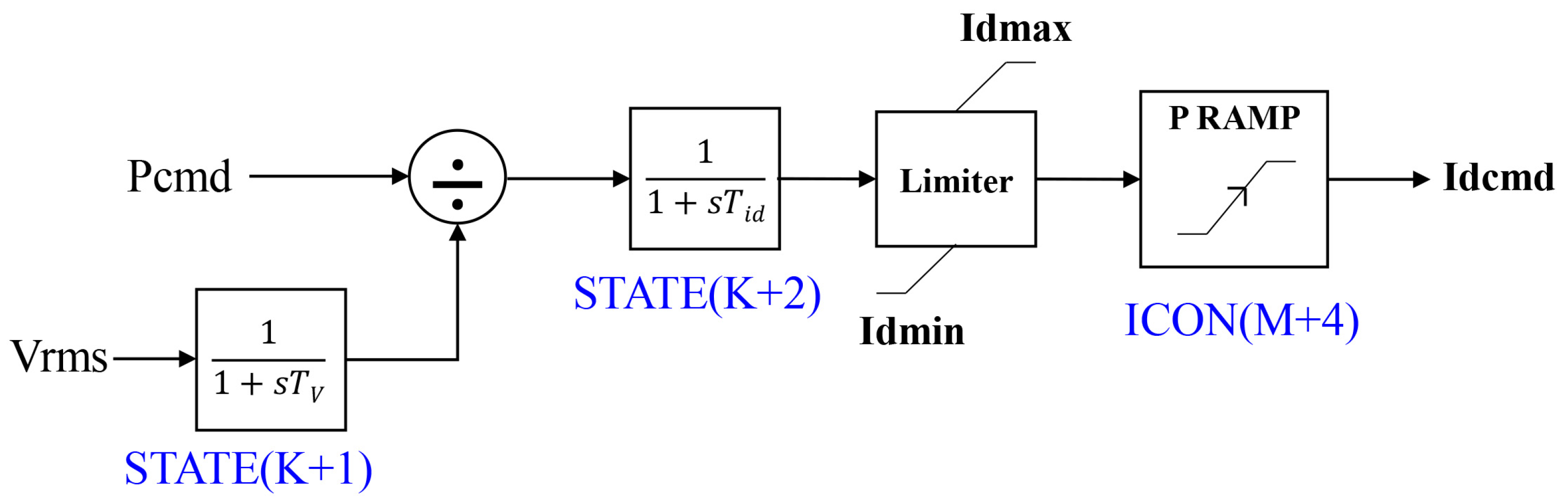
3.4. Active-Current-Control Part

The form and components of the active-current-control part are described in Figure 6 and

Table 4. Components in active-current-control part.

Pcmd [p.u.]	Active-power-control signal
Tv [s]	Voltage measurement filter time constant
Tf [s]	Frequency measurement filter time constant
Tid [s]	Active current filter time constant
Vrms [p.u.]	Voltage RMS value from grid
PFref	Power factor reference
STATE (K)	State variable for frequency filter
STATE (K + 1)	State variable for voltage filter
STATE (K + 2)	State variable for active current filter
Id_meas [p.u.]	Machine active-current output
Idmax [p.u.]	Maximum current for id
Idmin [p.u.]	Minimum current for id
Idcmd [p.u.]	Active current control signal to grid
Pramp [p.u.]/[s]	Ramp rate for power output
ICON (M + 4)	RAMPRATE_FLAG

. The primary function of this part is to convert the Pcmd received from the active-power-control part into Idcmd, the current injection signal. The current limiter and RAMP rate control in consideration of device performance belong to this part. A current output signal is generated using the received Pcmd and system voltage. After that, the limiter and ramp-rate control reflecting the device’s characteristics is performed, and the final Idcmd is generated after this process.

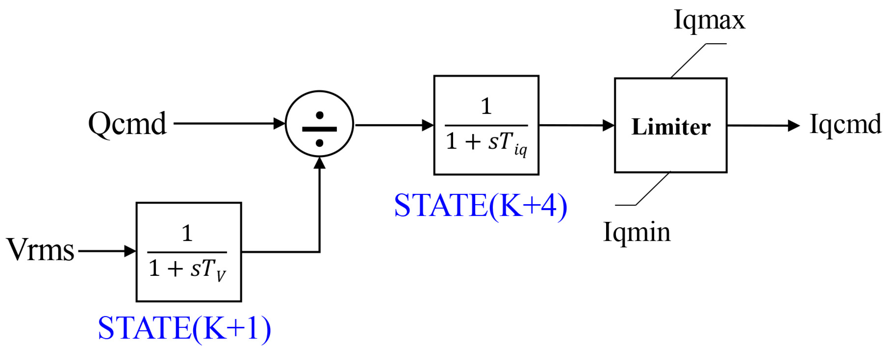
3.5. Reactive-Current-Control Part

The part that generates the reactive-current-control signal is described in Figure 7 and

Table 5. Components in reactive-current-control part.

Qcmd [p.u.]	Reactive-power-control signal
Tv [s]	Voltage measurement filter time constant
Tiq [s]	Reactive current filter time constant
Vrms [p.u.]	Voltage RMS value from grid
STATE (K + 1)	State variable for voltage filter
STATE (K + 4)	State variable for reactive current filter
Iq_meas [p.u.]	Machine reactive current output
Iqmax [p.u.]	Maximum current for iq
Iqmin [p.u.]	Minimum current for iq
Iqcmd [p.u.]	Reactive current control signal to grid

. The overall configuration is similar to the part that generates the active-current-control signal in Section 3.4. The main function of this part is to receive the signal from the reactive-power-control part and generate the reactive-power-current injection signal, Iqcmd. The previous part dealt with frequency and active power, but this part is different in that it is composed mainly of voltage and reactive power. Additional functions, such as the current limiter, are included in this part, so simulations can be performed by adding the necessary parameters to the dyr file.

4. Case Study

In this section, two case studies were performed for model validation. First, a test power system was used to verify the model’s characteristics. Afterward, to check whether the model operates normally in the general system, the developed model was put into the IEEE 14-bus system, and verification was attempted.

4.1. Model Validation in the Test System

4.1.1. Loadflow Simulation

Loadflow calculation is required before proceeding with dynamic simulation. For the developed ESS model test, loadflow calculation was performed in the test power system shown in Figure 8. The capacity of the ESS model used in the simulation was set to 1 (MVA). The test system is a small system consisting of five buses, two substations, and a single large machine.

4.1.2. Power-Control Mode

Each function included in the developed model was validated in this part. First, the active and reactive power output by power reference was checked. Simulations were performed using the settings and scenario described in

Table 6. Simulation settings for active-power control.

Function On/Off
All Switch	off
Initial Setting
Parameter	Value
P_ref [p.u.]	0.0
Q_ref [p.u.]	0.0
Scenario
Time [s]	Active-Power Reference [p.u.]
3	0 → 0.25
6	0.25 → 0.5
9	0.5 → 0.25
Time [s]	Rective-Power Reference [p.u.]
2	0 → 0.2
5	0.2 → 0.4
8	0.4 → 0.2

. If every function is turned off in the developed model, active- and reactive-power output is fixed according to the power reference value. Each function can be set using the ICON value. In PSS^®E, the electrical output of the machine is measured in units of p.u. The simulation was performed for 10 s, and the simulation results are shown in Figure 9. Simulation results show that the active and reactive power can be controlled independently.

4.1.3. Ramp-Rate-Control Mode

The output of ESS can be changed considering the ramp rate depending on the device’s characteristics. Therefore, the ESS simulation model that considers these characteristics is necessary for the transmission-level analysis. The developed ESS model in this paper can also handle ramp-rate control, and detailed references are given in Section 3.4. It is possible to select whether to apply the ramp-rate function using the ICON (M + 4) value in the developed model. The simulation settings for testing the ramp-rate control are described in

Table 7. Simulation settings for ramp-rate control.

Function On/Off
Ramp-Rate Switch	on
Initial Setting
Parameter	Value
P_ref [p.u.]	0.0
Pramp [p.u.]/[s]	0.25
Scenario
Time [s]	Active-Power Reference [p.u.]
1.0	0.0 → 1.0
6.0	1.0 → 0.0

, and the results can be seen in Figure 10. Since the output variation per second can be changed according to the ESS characteristics, the developed model allows this value to be set as a Pramp value. This simulation assumes that active-power output can change by 0.25 (p.u.) per second.

4.1.4. Power-Factor-Control Mode

There is a control method by the power factor in the ESS control requirements. It controls the ESS’s active and reactive power output by the power factor value at a constant ratio. This control method can also be used in our developed model, and the verification was carried out by setting it as shown in

Table 8. Simulation settings for pf control.

Function On/Off
Power-factor Switch	on
Initial Setting
Parameter	Value
P_ref [p.u.]	0.5
Q_ref [p.u.]	0.0
PF_ref	1.0
Scenario
Time [s]	Power-Factor Reference
1.0	1.0 → 0.8
5.0	0.8 → 1.0
8.0	1.0 → −0.8

. If the function is set as in Table 8, the reactive-power output is determined by the power factor based on the active-power value. Since the power factor has to consider both leading and lagging situations, negative power factors were also tested in the scenario. The simulation results are seen in Figure 11.

4.1.5. Deadband-Control Mode

The ESS can sense the system voltage and adjust the reactive-power output accordingly. When the system voltage fluctuates in a specific band based on the nominal voltage, the ESS does not respond to it. Therefore, it is necessary to set the deadband by reflecting these characteristics in simulations. The developed ESS simulation model includes a function that allows the user to set the deadband directly. The concept of the deadband is described in Figure 12.

The size of the deadband can be set using the Qdbd1 and Qdbd2 parameters. The numerical values used for the simulation and the scenario are shown in

Table 9. Simulation settings for deadband control.

Function On/Off
Pdroop Switch	on
Initial Setting
Parameter	Value
P_ref [p.u.]	0.5
Q_ref [p.u.]	0.0
Qdbd1, Qdbd2	0.01
Scenario
Time [s]	PCC voltage [p.u.]
0.0~1.0	1.001
1.0~2.0	0.998
2.0~3.0	0.995
3.0~4.0	0.993
4.0~5.0	0.990
5.0~6.0	0.987
6.0~7.0	0.985
7.0~8.0	0.983
8.0~9.0	0.980
9.0~10.0	0.977

, and the simulation results are seen in Figure 13. The ESS does not respond to system voltage when the voltage is between 1.0 and 0.99 (p.u.). However, when the voltage is out of the band, the reactive power output of the developed model changes accordingly.

4.2. Model Verification in the IEEE 14-Bus System

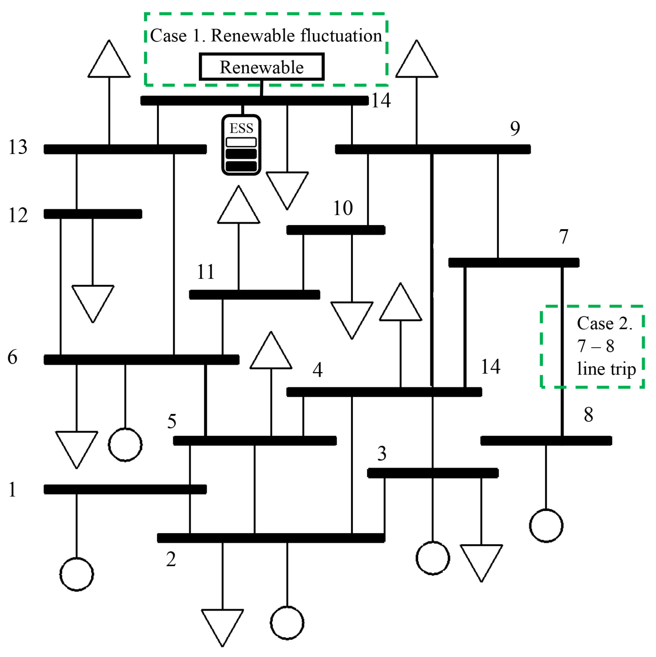
As mentioned earlier, in Section 2.1, some applications exploit ESS in the power system. In this section, the developed ESS model is verified after setting up the system conditions assuming two situations in the power system. In the previous case, Section 4.1, the regular operation of the developed ESS analysis model was verified by testing in the simple power system. In this section, the developed model was put into the IEEE 14-bus system to check whether it operates well in a general power system. The IEEE 14-bus system is a verified system which has been used in power system analysis for a long time. In addition this system is not too large, so it is suitable to see the response of the ESS. The form of the IEEE 14-bus system with information on each case is shown in Figure 14.

4.2.1. Loadflow Simulation

Since the IEEE 14-bus system is a kind of proven power system, there is no doubt about the loadflow calculation of this system. In this study, the system was modified by inputting additional elements, such as a renewable plant. After setting each element of the system properly for the convergence of the loadflow calculation, those results were used for dynamic simulation for each scenario.

4.2.2. Case 1. Mitigation of Power Fluctuations

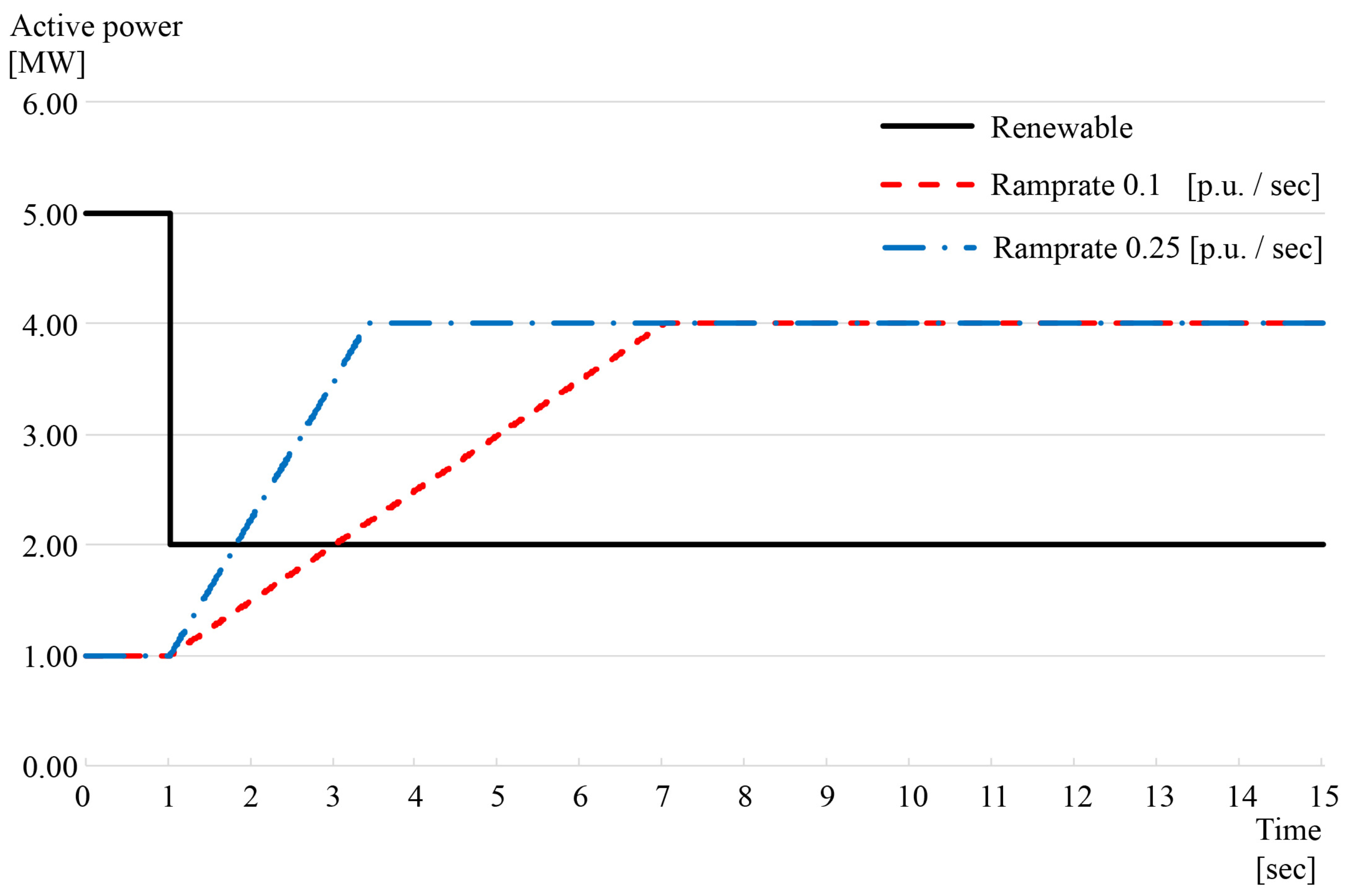
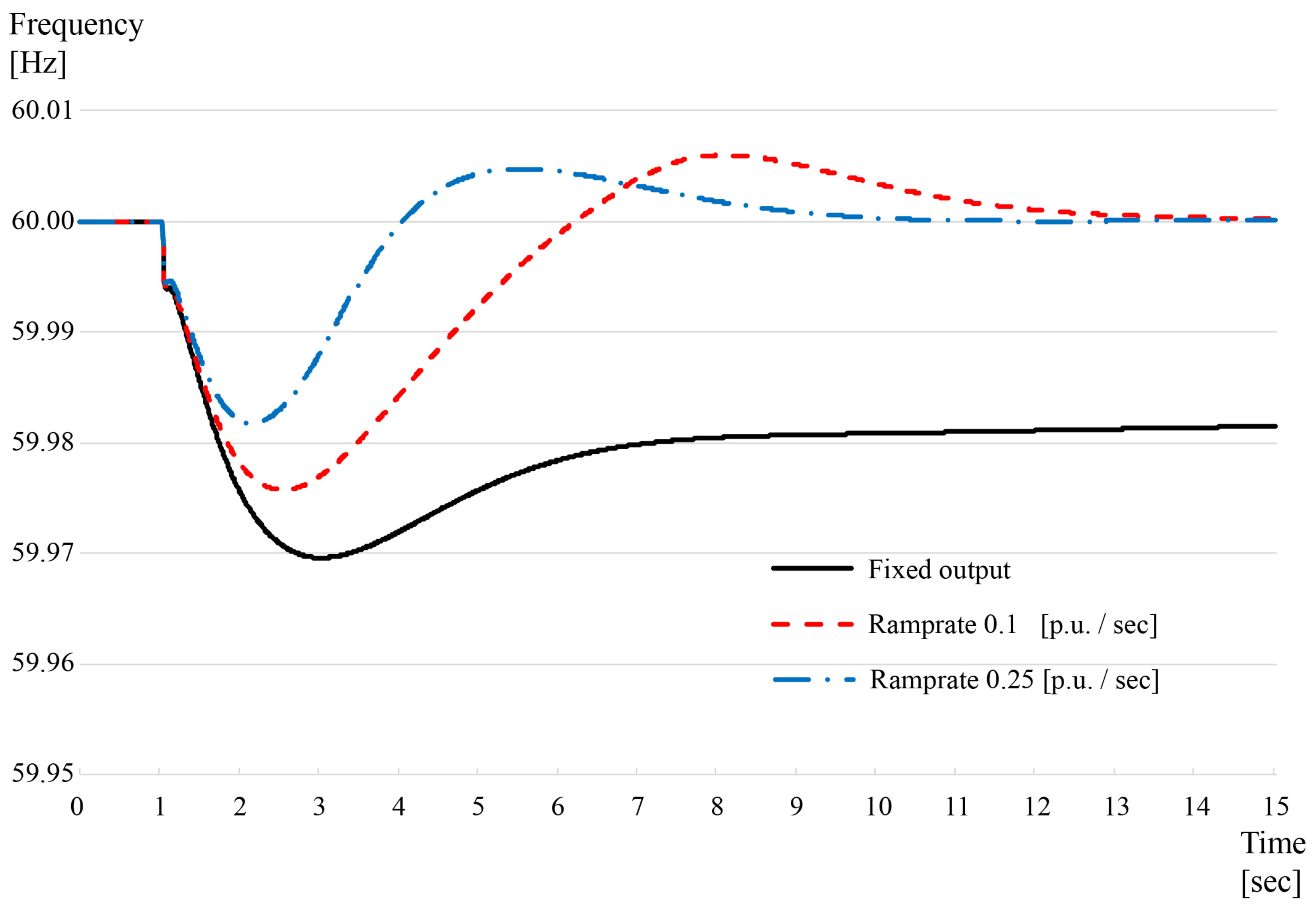
Case 1 uses a scenario in which the system is affected by power fluctuations in a renewable power plant. This scenario assumes that the renewable power plant and ESS are integrated on bus 14, relatively far from the other generators. When renewable power fluctuates, ESS plays a role in mitigating the fluctuation. The details of the scenario are as follows. In the simulation, the initial output of the ESS was 1 (MW), and the output of the renewable plant decreased by 3 (MW) at 1 (s). After that, the ESS was set to increase the power output up to 4 (MW). The total capacity of the ESS was set to 5 (MVA), slightly larger than the fluctuation amount so that it could sufficiently respond to the change amount. The simulation was performed for 15 (s), and the reactive power output of the ESS was fixed during this process. Since the power capacity of each ESS is different in reality, the analysis model should be able to set the ramp rate differently. In the simulation, the ramp rate was set to 0.1 and 0.25, respectively, and the developed model was checked to confirm if it worked properly. Figure 15 shows the change in the active-power output of the renewable power plant and ESS. There are some variations in the output according to the ramp-rate setting in Figure 15. Figure 16 shows the frequency fluctuations measured on bus 14 under the same conditions. Since the active-power output in the renewable plant and ESS is not large, the absolute frequency value is not significant in this case. However, there are some positive effects of ESS in Figure 16, clearly.

4.2.3. Case 2. Frequency Regulation

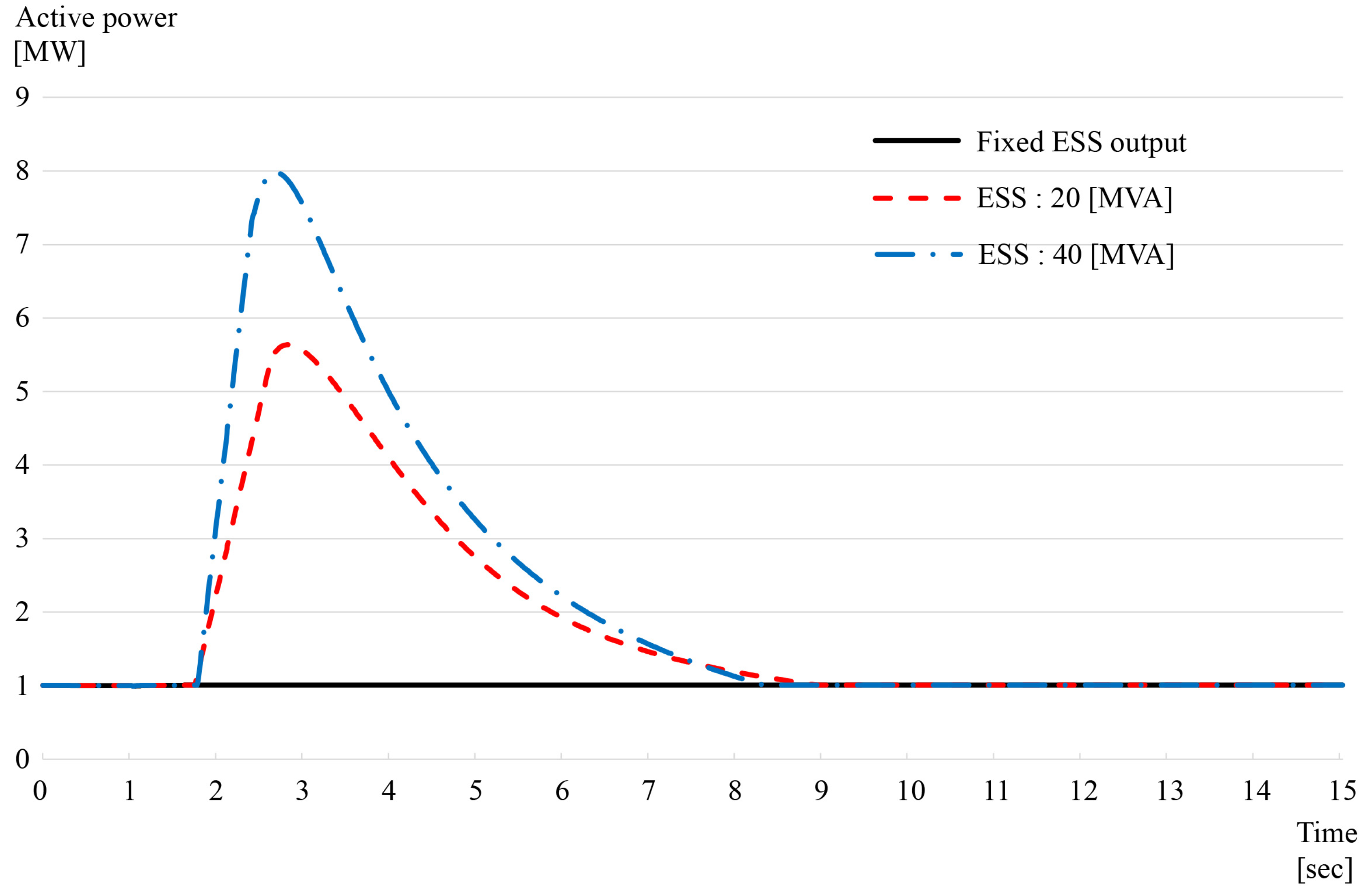
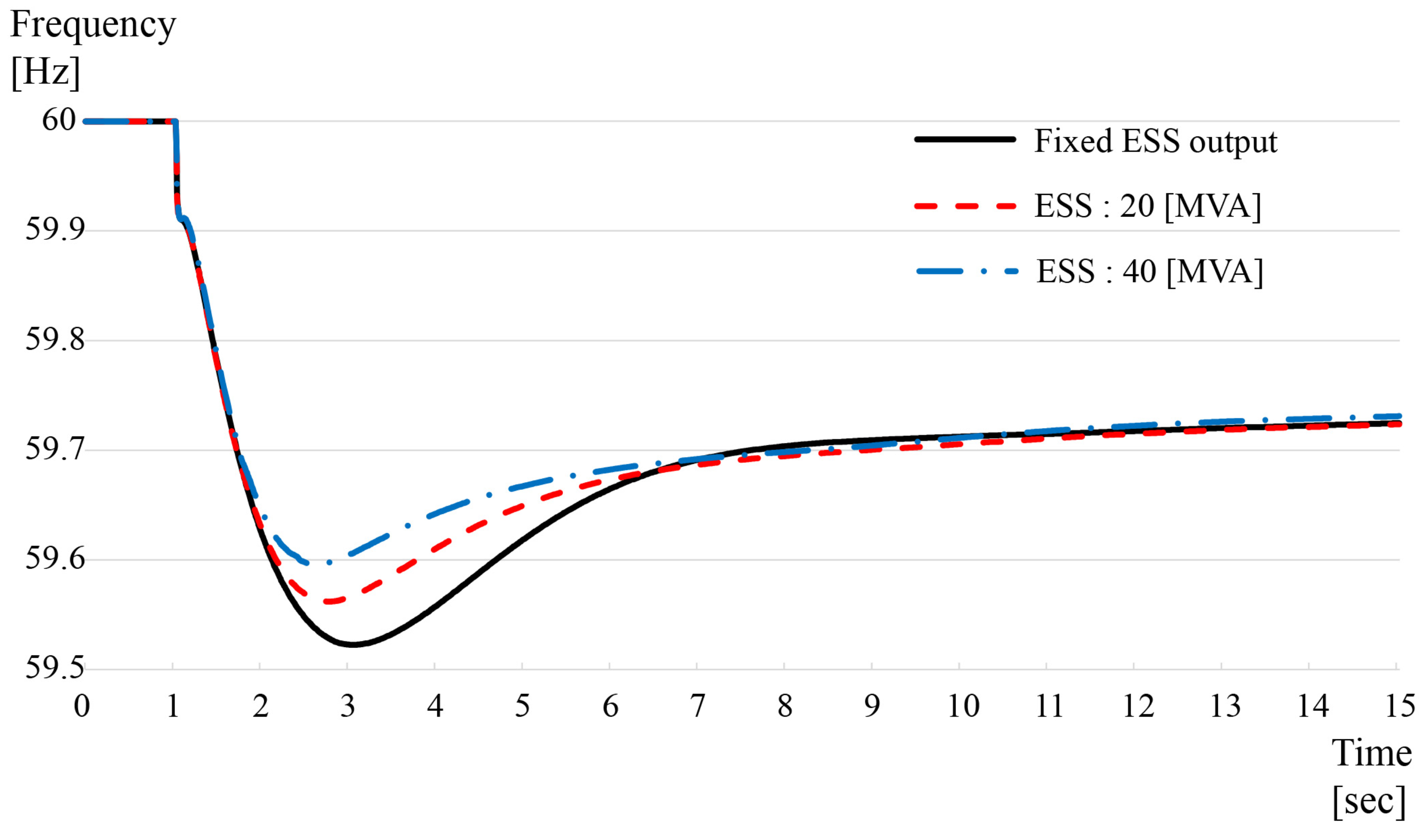
FR function of the developed ESS model is verified in case 2. When a fault occurs in a system, the frequency may fluctuate significantly. In this case, it was confirmed whether the ESS could normally regulate the frequency fluctuations. Case 2 used the same IEEE14-bus system as case 1, and the line-trip contingency (between bus 7 and 8) was selected as a simulation scenario. Figure 14 shows that this accident dramatically affects the system because the fault also trips the generator. The power output of the generator are 35 (MW) and 10 (MVAr), repectively. In order to cope with the loss of power, the output of other generators and ESS in the system is increased. In general, the frequency tends to fluctuate throughout the whole power system. Therefore, it is difficult to see the effect on the frequency with a small variation in active power output. Therefore, case-2 simulations were conducted by setting the ESS capacity to 20 and 40 (MVA), respectively. The active power with which the ESS responds to the fault is shown in Figure 17. When the ESS model detects a decrease in frequency, the 20 (MVA) ESS outputs up to 5.7 (MW), and the 40 (MVA) capacity ESS outputs up to 8 (MW) instantaneously. The fluctuation in the frequency measured on bus 14 can be seen in Figure 18. If the output of the ESS was fixed, the frequency dropped to 59.52 (Hz), and the FR function worked clearly as the input capacity of the ESS increased.

5. Conclusions

Although various ESS models have been proposed in previous studies, there are some non-critical elements for transmission-level power-system analysis. This research developed an ESS analysis model that can be used in commercial programs. The developed model is suitable for transmission-level analysis, and it is easy to use because it shows a relatively uncomplicated configuration compared to the previous models. The programming language Fortran is used to compile the analysis model code. The detailed configuration of the developed model was described using block diagrams and tables. Simulations were performed for four modes to verify the developed model in the test system. In order to verify that the developed model operates properly in a general system, a simulation was performed in the IEEE 14-bus power system, and the result was confirmed. The developed ESS model can be used for power-system analysis, and it can be used as reference material for model development. In future work, the detailed aspects of the ESS analysis model will be upgraded, and it will be used for various case studies, including stability analysis.

References

- Zhao, H.; Wu, Q.; Hu, S.; Xu, H.; Rasmussen, C.N. Review of energy storage system for wind power integration support. Appl. Energy 2015, 137, 545–553. [Google Scholar] [CrossRef]
- Tian, Y.; Bera, A.; Benidris, M.; Mitra, J. Stacked revenue and technical benefits of a grid-connected energy storage system. IEEE Trans. Ind. Appl. 2018, 54, 3034–3043. [Google Scholar] [CrossRef]
- Faisal, M.; Hannan, M.A.; Ker, P.J.; Hussain, A.; Mansor, M.B.; Blaabjerg, F. Review of energy storage system technologies in microgrid applications: Issues and challenges. IEEE Access 2018, 6, 35143–35164. [Google Scholar] [CrossRef]
- Wong, L.A.; Ramachandaramurthy, V.K.; Taylor, P.; Ekanayake, J.; Walker, S.L.; Padmanaban, S. Review on the optimal placement, sizing and control of an energy storage system in the distribution network. J. Energy Storage 2019, 21, 489–504. [Google Scholar] [CrossRef]
- Arani, A.K.; Karami, H.; Gharehpetian, G.; Hejazi, M. Review of Flywheel Energy Storage Systems structures and applications in power systems and microgrids. Renew. Sustain. Energy Rev. 2017, 69, 9–18. [Google Scholar] [CrossRef]
- Faraji, F.; Majazi, A.; Al-Haddad, K. A comprehensive review of flywheel energy storage system technology. Renew. Sustain. Energy Rev. 2017, 67, 477–490. [Google Scholar]
- Sharma, P.; Kumar, V. Current technology of supercapacitors: A review. J. Electron. Mater. 2020, 49, 3520–3532. [Google Scholar] [CrossRef]
- Liu, S.; Wei, L.; Wang, H. Review on reliability of supercapacitors in energy storage applications. Appl. Energy 2020, 278, 115436. [Google Scholar] [CrossRef]
- Hu, Z. Energy Storage for Power System Planning and Operation; John Wiley & Sons: Hoboken, NJ, USA, 2020. [Google Scholar]
- Budt, M.; Wolf, D.; Span, R.; Yan, J. A review on compressed air energy storage: Basic principles, past milestones and recent developments. Appl. Energy 2016, 170, 250–268. [Google Scholar] [CrossRef]
- Olabi, A.; Wilberforce, T.; Ramadan, M.; Abdelkareem, M.A.; Alami, A.H. Compressed air energy storage systems: Components and operating parameters—A review. J. Energy Storage 2021, 34, 102000. [Google Scholar] [CrossRef]
- Sutanto, D.; Cheng, K.W.E. Superconducting magnetic energy storage systems for power system applications. In Proceedings of the 2009 International Conference on Applied Superconductivity and Electromagnetic Devices, Chengdu, China, 25–27 September 2009; pp. 377–380. [Google Scholar]
- Xu, N.; Li, X.; Zhao, X.; Goodenough, J.B.; Huang, K. A novel solid oxide redox flow battery for grid energy storage. Energy Environ. Sci. 2011, 4, 4942–4946. [Google Scholar] [CrossRef]
- Winsberg, J.; Janoschka, T.; Morgenstern, S.; Hagemann, T.; Muench, S.; Hauffman, G.; Gohy, J.F.; Hager, M.D.; Schubert, U.S. Poly (TEMPO)/Zinc Hybrid-Flow Battery: A Novel, “Green”, High Voltage, and Safe Energy Storage System. Adv. Mater. 2016, 28, 2238–2243. [Google Scholar] [CrossRef] [PubMed]
- Cao, J.; Emadi, A. A new battery/ultracapacitor hybrid energy storage system for electric, hybrid, and plug-in hybrid electric vehicles. IEEE Trans. Power Electron. 2011, 27, 122–132. [Google Scholar]
- Zhang, L.; Hu, X.; Wang, Z.; Sun, F.; Deng, J.; Dorrell, D.G. Multiobjective optimal sizing of hybrid energy storage system for electric vehicles. IEEE Trans. Veh. Technol. 2017, 67, 1027–1035. [Google Scholar] [CrossRef]
- Babu, T.S.; Vasudevan, K.R.; Ramachandaramurthy, V.K.; Sani, S.B.; Chemud, S.; Lajim, R.M. A comprehensive review of hybrid energy storage systems: Converter topologies, control strategies and future prospects. IEEE Access 2020, 8, 148702–148721. [Google Scholar] [CrossRef]
- Leon, J.I.; Dominguez, E.; Wu, L.; Alcaide, A.M.; Reyes, M.; Liu, J. Hybrid energy storage systems: Concepts, advantages, and applications. IEEE Ind. Electron. Mag. 2020, 15, 74–88. [Google Scholar] [CrossRef]
- Mohamad, F.; Teh, J.; Lai, C.M.; Chen, L.R. Development of energy storage systems for power network reliability: A review. Energies 2018, 11, 2278. [Google Scholar] [CrossRef] [Green Version]
- Poolla, B.K.; Bolognani, S.; Dörfler, F. Optimal placement of virtual inertia in power grids. IEEE Trans. Autom. Control 2017, 62, 6209–6220. [Google Scholar] [CrossRef] [Green Version]
- Golpîra, H.; Atarodi, A.; Amini, S.; Messina, A.R.; Francois, B.; Bevrani, H. Optimal energy storage system-based virtual inertia placement: A frequency stability point of view. IEEE Trans. Power Syst. 2020, 35, 4824–4835. [Google Scholar] [CrossRef]
- Adewumi, O.B.; Fotis, G.; Vita, V.; Nankoo, D.; Ekonomou, L. The Impact of Distributed Energy Storage on Distribution and Transmission Networks’ Power Quality. Appl. Sci. 2022, 12, 6466. [Google Scholar] [CrossRef]
- Calero, F.; Cañizares, C.A.; Bhattacharya, K.; Anierobi, C.; Calero, I.; de Souza, M.F.Z.; Farrokhabadi, M.; Guzman, N.S.; Mendieta, W.; Peralta, D.; et al. A Review of Modeling and Applications of Energy Storage Systems in Power Grids. Proc. IEEE 2022. [Google Scholar] [CrossRef]
- Carnegie, R.; Gotham, D.; Nderitu, D.; Preckel, P.V. Utility Scale Energy Storage Systems: Benefits, Applications, and Technologies. State Utility Forecasting Group. Technical Report. 2013. Available online: https://www.purdue.edu/discoverypark/energy/assets/pdfs/SUFG/publications/SUFG%20Energy%20Storage%20Report.pdf (accessed on 4 November 2022).
- Koohi-Kamali, S.; Tyagi, V.; Rahim, N.; Panwar, N.; Mokhlis, H. Emergence of energy storage technologies as the solution for reliable operation of smart power systems: A review. Renew. Sustain. Energy Rev. 2013, 25, 135–165. [Google Scholar] [CrossRef]
- Vazquez, S.; Lukic, S.M.; Galvan, E.; Franquelo, L.G.; Carrasco, J.M. Energy storage systems for transport and grid applications. IEEE Trans. Ind. Electron. 2010, 57, 3881–3895. [Google Scholar] [CrossRef] [Green Version]
- Roberts, B.P.; Sandberg, C. The role of energy storage in development of smart grids. Proc. IEEE 2011, 99, 1139–1144. [Google Scholar] [CrossRef]
- Cañizares, C.A.; Bhattacharya, K.; Sohm, D. Frequency regulation model of bulk power systems with energy storage. IEEE Trans. Power Syst. 2021, 37, 913–926. [Google Scholar]
- Nasrazadani, H.; Sedighi, A.; Seifi, H. Enhancing long-term voltage stability of a power system integrated with large-scale photovoltaic plants using a battery energy storage control scheme. Int. J. Electr. Power Energy Syst. 2021, 131, 107059. [Google Scholar] [CrossRef]
- Beaudin, M.; Zareipour, H.; Schellenberglabe, A.; Rosehart, W. Energy storage for mitigating the variability of renewable electricity sources: An updated review. Energy Sustain. Dev. 2010, 14, 302–314. [Google Scholar] [CrossRef]
- Siemens PTI. PSS®E 34 Model Library; Siemens PTI: Schenectady, NY, USA, 2015. [Google Scholar]
- PowerWorld Simulator. Available online: https://www.powerworld.com/files/Block-Diagrams-18.pdf (accessed on 18 March 2021).
- Siemens PTI. PSS®E 34 Program Operation Manual; Siemens PTI: Schenectady, NY, USA, 2015. [Google Scholar]
- Siemens PTI. PSS®E 34 Program Application Guide; Siemens PTI: Schenectady, NY, USA, 2015. [Google Scholar]
- Operational Analysis and Engineering, AEMO. Power System Model Guidelines. 2018. Available online: https://aemo.com.au/-/media/Files/Electricity/NEM/Security_and_Reliability/System-Security-Market-Frameworks-Review/2018/Power_Systems_Model_Guidelines_PUBLISHED.pdf (accessed on 18 March 2021).
- IEEE 14-Bus System. Available online: https://icseg.iti.illinois.edu/ieee-14-bus-system (accessed on 27 November 2022).
Figure 1.
Schematic diagram of ESS analysis model.
Figure 3.
Schematic diagram of the developed ESS analysis model.
Figure 4.
Diagram of active-power-control part.
Figure 5.
Diagram of reactive-power-control part.
Figure 6.
Diagram of active-current-control part.
Figure 7.
Diagram of reactive-current-control part.
Figure 8.
Test system for the developed ESS model.
Figure 9.
Simulation results: power reference.
Figure 10.
Simulation results: ramp rate.
Figure 11.
Simulation results: power factor.
Figure 12.
Deadband concept in the developed model.
Figure 13.
Simulation results: deadband.
Figure 14.
IEEE 14-bus system with case-study scenario information.
Figure 15.
Results (case. 1: renewable variation): active-power fluctuations.
Figure 16.
Results (case. 1: renewable variation): frequency fluctuations.
Figure 17.
Results (case. 2: line trip): active-power fluctuations.
Figure 18.
Results (case. 2: line trip): frequency fluctuations.