Article

Feasibility of Photovoltaic Module Single-Diode Model Fitting to the Current–Voltage Curves Measured in the Vicinity of the Maximum Power Point for Online Condition Monitoring Purposes

by
Heidi Kalliojärvi
*,
Kari Lappalainen
and
Seppo Valkealahti
Electrical Engineering Unit, Tampere University, P.O. Box 692, 33101 Tampere, Finland
*
Author to whom correspondence should be addressed.
Energies 2022, 15(23), 9079; https://doi.org/10.3390/en15239079
Submission received: 5 November 2022 / Revised: 23 November 2022 / Accepted: 26 November 2022 / Published: 30 November 2022

Abstract

:

Highlights

What are the main findings?
  • Single-diode model fitting to partial IU curves was systematically investigated.
  • The IU curves were measured in the vicinity of the MPP.
  • The IU curve region selected for fitting had a significant effect on the fit accuracy.
What is the implication of the main finding?
  • Suitably constructed partial IU curves can be used in online condition monitoring.
  • PV module aging can be detected and quantified using partial IU curves.

Abstract

Photovoltaic system condition monitoring can be performed via single-diode model fitting to measured current–voltage curves. Model parameters can reveal cell aging and degradation. Conventional parameter identification methods require the measurement of entire current–voltage curves, causing interruptions in energy production. Instead, partial curves measured near the maximum power point offer a promising option for online condition monitoring. Unfortunately, measurement data reduction affects fitting and diagnosis accuracy. Thus, the optimal selection of maximum power point neighbourhoods used for fitting requires a systematic analysis of the effect of data selection on the fitted parameters. To date, only one published article has addressed this issue with a small number of measured curves using symmetrically chosen neighbourhoods with respect to the maximum power. Moreover, no study has determined single-diode fit quality to partial curves constructed via other principles, e.g., as a percentage of the maximum power point voltage. Such investigation is justified since the voltage is typically the inverter reference quantity. Our work takes the study of this topic to a whole new scientific level by systematically examining how limiting the current–voltage curve measuring range to maximum power point proximity based on both power and voltage affects single-diode model parameters. An extensive dataset with 2400 measured curves was analysed, and statistically credible results were obtained for the first time. We fitted the single-diode model directly to experimental curves without measuring outdoor conditions or using approximations. Our results provide clear guidance on how the choices of partial curves affect the fitting accuracy. A significant finding is that the correct selection of maximum power point neighbourhoods provides promising real-case online aging detection opportunities.

1. Introduction

The photovoltaic (PV) single-diode model applied to the measured current–voltage (IU) curves of the PV module provides a valuable tool for monitoring and diagnosing the condition of a PV system. Every IU curve is characterized by a set of single-diode model parameters. Changes in these parameters can reveal changes in the condition of the PV module. Among the parameters, series resistance is especially useful in the detection of PV module aging and degradation [1,2]. The single-diode model parameters are obtained from measured IU curves using a mathematical fitting procedure. Parameter identification techniques can be divided into offline and online techniques. The conventional offline parameter identification techniques require the measurement of the entire IU curve, including its open-circuit (OC) and short-circuit (SC) ends. Unfortunately, this requires the PV system to be shut down for the period of diagnostic measurements, accompanied with power losses and undesired interruptions in electricity production. In contrast, online identification techniques utilizing only partially measured IU curves are designed to avoid such interruptions. Therefore, online condition monitoring and diagnosis methods are strongly preferred in practical PV systems, and their development needs to be vastly enhanced.
The practical requirement for single-diode model online parameter identification techniques is that the operating point does not need to move too far from the maximum power point (MPP). The reduction in measurement data available for curve fitting implies a compromise in the fit quality; single-diode model parameters obtained from a partial IU curve measured in the vicinity of the MPP tend to suffer from lower accuracy. This holds especially for the series resistance parameter, which is extremely important in aging diagnostics. This issue raises the following yet unanswered questions: (1) how large should the proportion of the IU curve measured for fitting be to maintain the sufficient accuracy of the identified parameters and (2) how should the MPP environment be selected for analysis so that all parameters, especially the series resistance, are identified with sufficient accuracy? For the first time, these questions are answered in a comparative and statistically plausible manner in the present study.
In the literature, some light has been shed on the described problematics. Several authors, having first applied their developed IU curve fitting procedures to the entire curve, also tested the capability of the procedure using partial IU curves. The choice of the used partial IU curves varied from author to author. The authors of [3] showed an example of fitting the model to a partial IU curve obtained by moving 3 V to both sides from the MPP voltage (UMPP) of a PV module. Consequently, the entire OC slope of the IU curve became well repeated, while the SC slope of the fitted curve overshot clearly. Alternatively, the authors suggested choosing the neighbourhood symmetrically with respect to the MPP power (PMPP) and presented an example where the IU curve cutting limit was 90% of PMPP. Such cutting made the fitted series resistance increase and the shunt resistance decrease compared with the values obtained using the entire curve. In [4], partial IU curves were formed by selecting 30% of the measurement points closest to the MPP for fitting. The fitting test performed under high-irradiance conditions (with high irradiance being the optimal operating region to guarantee the proper performance of the single-diode model and especially series resistance identification [1]), revealed that the partial IU curve produced smaller series resistance values than the entire curve. The normalized root mean square errors (nRMSEs) were approximately 2% and 5% for the entire and partial curves in [4], respectively. The authors of [5] also validated their curve fitting method to partial IU curves using 50% of the measurement points, selecting those closest to the MPP. It was found that their curve fitting method performed well also in the case of such partial IU curves. The author of [6] investigated the usability of their model with partial IU curves by choosing measurement points so that the ratio between the highest voltage values of the partially and the fully measured curves was around 90% and the ratio between highest current values of the partial and full curves was around 98%. The fitting was observed to perform acceptably in such cases. However, showing only one or a few examples of constructing partial IU curves is not sufficient to find an optimal way to measure partial IU curves in the vicinity of the MPP for fitting. In order to rectify this shortcoming, the present paper exploits an exactly determined systematic approach for that purpose. Indeed, partial IU curves constructed step by step starting from the full IU curve are used in this study. This approach enables a consistent analysis of the effect of the selection of the measurement region on the fit, which in turn guarantees the usability of the obtained results for further theoretical analyses as well as real practical applications in the condition monitoring of PV systems.
Some studies have compared the effect of the location of special points picked around the MPP for fitting. The authors of [7] picked four points in the vicinity of the MPP for single-diode model fitting and investigated the effect of the location of the selected points on the fit quality. The authors found that the optimal trade-off was obtained by selecting two points from both sides of the MPP. Such a configuration allowed them to capture the exponential curvature around the MPP correctly, resulting in equally good fit qualities in the OC and SC ends of the IU curve. In [8], it was observed that eight measurement points with a spacing of 1 V were sufficient to capture the MPP curvature of a PV module. The authors justified this with two observations. Firstly, a 15% voltage reduction to the left of the MPP voltage was noticed to be usually sufficient to reach the almost linear high-current region of the IU curve. Secondly, test points up to 60–75% of the MPP current (IMPP) were selected on the right side of the MPP as suggested in [2] to properly identify series resistance. The fitting test performed under high-irradiance conditions provided good results, although the power was only reduced by less than 11% of PMPP. In [9,10], six points divided into two three-point blocks were chosen around the MPP. In [10], it was observed that the voltage separation of the points in the same block should not exceed 5% of the first selected voltage point. In addition, the difference between the central points of the two blocks should be less than 20% of the voltage at the central point of the first block. When the voltage steps determining the density of the selected points were chosen as 2% of UMPP [9], the OC end of the fitted curve overshot clearly, and the SC end undershot slightly. However, setting the voltage steps as 2.5% of UMPP significantly improved the fit quality, causing only a slight undershoot at the OC end of the fitted curve and an overshoot at the OC end. The authors of [11] also adopted the principle of the point selection strategy of [9,10], but the location of the six points selected for fitting was sparser. The authors of [12] used four arbitrary points on the IU curve jointly with the slopes of the IU curve at these points. The four points were selected differently for different tests. The presented method worked even when restricting the IU curve in the vicinity of the MPP at voltage limits of about 2–3% of UMPP. However, all the above studies only used some special points picked around the MPP for fitting, and a comprehensive picture and a systematic analysis of the effects of constructing a partial IU curve on fitting accuracy were lacking. In contrast, point selection for fitting is performed in the present study in a manner that is computationally systematic and also comparable on a wider scale.
What all the above studies have in common is that they mainly examined the fitting of the single-diode model only in certain cases of partial IU curves, i.e., by means of examples. To the best of our knowledge, there exists only one published research paper [13] in which the measured IU curve was piecewise cut into a smaller portion and the effects of cutting on the fitted single-diode model parameters were investigated. It was found that the identification of the single-diode model parameters and outdoor conditions performed well even in close vicinity of the MPP. Such an observation is crucial for the online identification of the model parameters. Unfortunately, in [13], the identification of the single-diode model parameters was studied with only a small number of 20 IU curves based on PMPP percentages, and there exists no similar study with a larger number of data that provides statistically plausible results. Moreover, no IU curve cutting methods other than cutting based on PMPP percentages have been investigated in a systematic manner. Both shortcomings are extremely important for the development of the online condition monitoring of photovoltaic systems and are concisely addressed in this work.
The present paper provides a systematic study on how limiting the measurement region to partial IU curves in the vicinity of the MPP affects the accuracy of the fitted single-diode model parameters. The analysis is based on numerous data, with 2400 measured current–voltage curves, thus employing many more data than the analyses in earlier studies; therefore, this study is the only one providing statistically plausible results. The raw measurement data obtained with the I
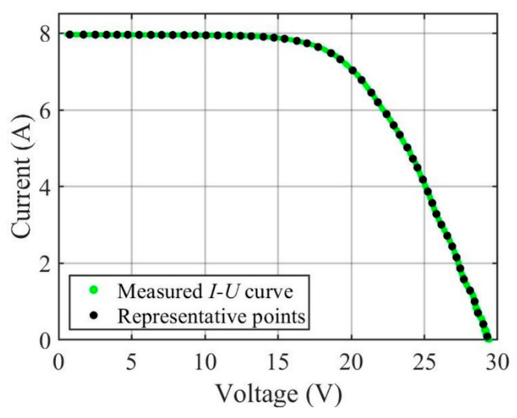
U curve tracer were processed using an advanced procedure: First, we removed abnormal measurement points; then, we distributed a fixed number of IU points evenly along the IU curve, as in [14]. In this way, the correct weight of the different parts of the IU curve was ensured, resulting in comparable results in each case studied. The selection of partial IU curves was made using two alternative methods based on MPP power and MPP voltage. The latter method is systematically studied for the first time in this work. We also developed an advanced theoretical model and a procedure to fit the single-diode model directly to the measured IU curves without the need to measure additional quantities, such as temperature or irradiance, or to use approximative fitting methods. Finally, the parameter values of the single-diode model obtained under certain irradiance and temperature conditions were converted to comparable values under standard test conditions (STCs).
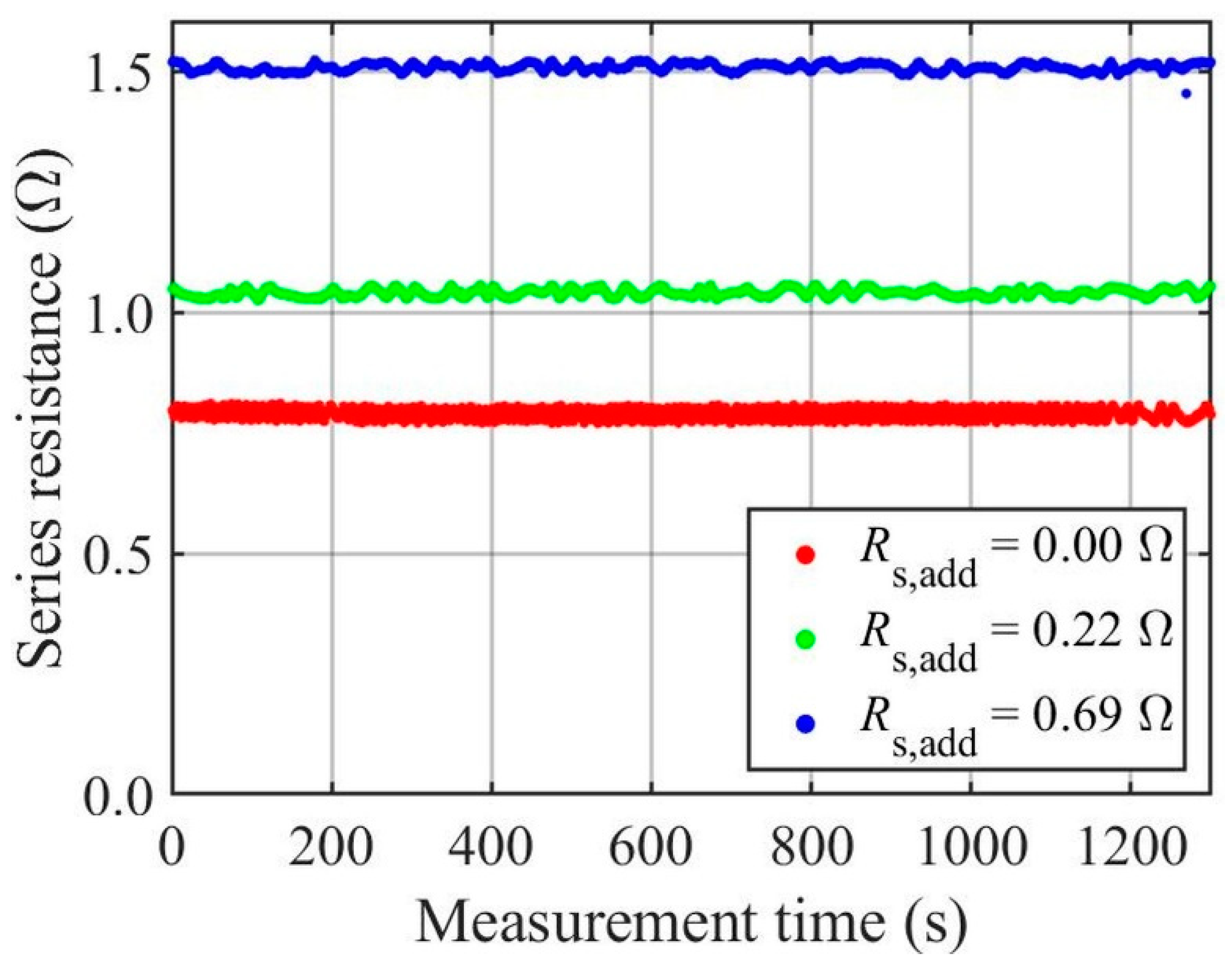
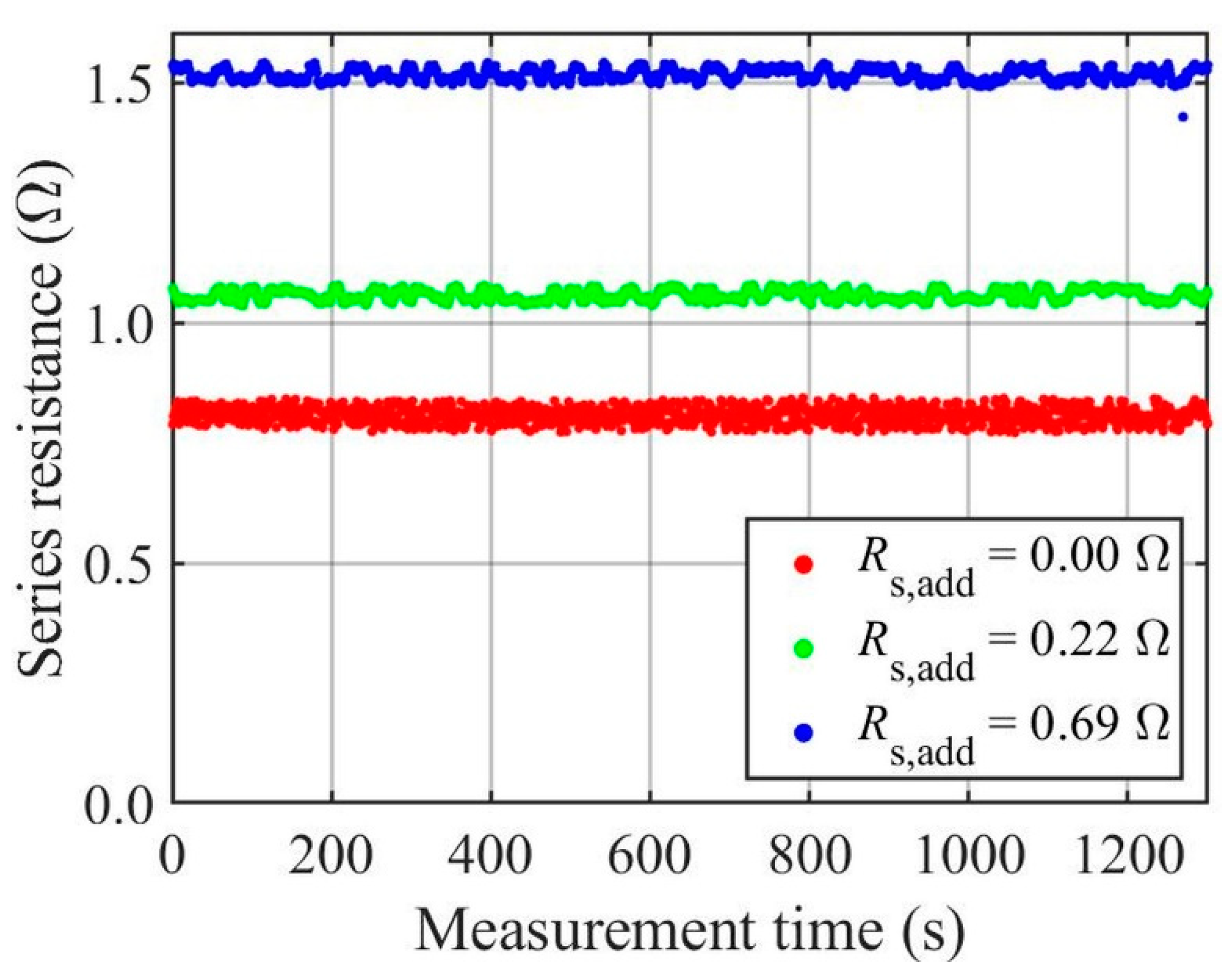
The novelty of this work lies in both its theoretical and practical applicability to the condition monitoring of PV systems. Groundbreakingly, the results of the study provide clear guidance on how the choice of the partial IU curve affects the accuracy of the parameters of the fitted single-diode model. Such relation is investigated in the present study for the first time. A very significant finding is that a correct selection of the vicinity of the maximum power point for fitting provides a promising opportunity to detect aging in real applications. Series resistance is a key quantity for aging detection, and we further investigated how the increase in the number of IU curves used for fitting improves the accuracy of the identified average parameter value. Such information is of practical relevance when designing any IU curve-based condition monitoring approach. As a final step, the suitability of the used single-diode model fitting procedure for PV module aging detection was demonstrated by utilizing full and partial IU curves measured with additional series resistances. The findings clearly outline the correct selection of partial IU curves used for aging detection.
The remainder of the paper is organized as follows: Section 2 provides information about the mathematical single-diode model jointly with the used iterative fitting procedure; then, the used data and their pre-processing procedure are introduced. The presentation of the two different IU curve cutting methods completes Section 2. In Section 3, the experimental results are presented and discussed. Finally, Section 4 closes the paper.

2. Methods and Data

2.1. Used Electrical Model and Fitting Procedure

The single-diode model, which is widely used for describing the IU characteristics of a PV module [15], is also used in this work.
I = I ph I o ( exp ( U + IR s AU T ) 1 ) U + IR s R h ,
where Iph is the photogenerated current, Io is the dark saturation current, and A is the diode ideality factor. As in [16], A is considered constant with a value of 1.1. The two parasitic resistances, series resistance Rs and shunt resistance Rh, account for the different loss mechanisms occurring in the PV cell. UT = NskBT/q is the thermal voltage, where Ns is the number of PV cells connected in series, kB is the Boltzmann constant, T is the PV cell operating temperature, and q is the electron charge.
The fitting procedure utilized in the present work was initially presented in [16]. It takes the measured IU curves and the STC electrical characteristics of the PV module as its inputs. The outputs are the single-diode model parameters (Iph, Io, Rs, and Rh) and the operating conditions (G and T), with G being the irradiance. No preliminary information of the outdoor conditions is needed. The direct output parameters are (Iph, Rs, Rh, and T). Io is calculated inside the fitting function called fit.m in Matlab using the following equation:
I o = I ph U OC R h exp ( AU T U OC ) 1          
derived from (1) in the OC. In (2), the OC voltage is obtained as in [17] as
  U OC = U OC ,   STC + K U ( T T STC ) + AU T ln ( G eff ) ,  
where UOC,STC is the OC voltage in under STCs, KU is the temperature coefficient of UOC, and TSTC is the STC temperature of 25 °C. The efficient irradiance, Geff, is calculated as
  G eff = I SC I SC ,   STC + K I ( T T STC ) ,    
where short-circuit current ISC is approximated to be equal to the photocurrent obtained by the fitting, ISC, STC is the SC current under STCs, and KI is the temperature coefficient of ISC. The irradiance is calculated after the actual fitting as
  G = G STC I SC I SC ,   STC + K I ( T T STC ) ,  
where GSTC is the STC irradiance of 1 kW/m2. The short-circuit current is obtained from the fitted curve as
I SC = I ph 1 + R s R h .
Finally, the investigated model parameter values are converted to STCs using the formulae [18,19]
I ph ,   STC = G STC I ph G K I ( T T STC )  
and
R s ,   STC = R s .
In particular, the choice of Formula (8) was justified in [18], where the temperature dependence of series resistance was also observed, but with minor significance. Other parameters can also be also converted to STCs [18,19,20]. However, this is out of the scope of the present paper, which focuses mainly on aging detection, and they are thus omitted.
The computational costs of the used iterative fitting procedure can be evaluated as the number of iterations jointly with the number of times in which the objective function is evaluated during the fitting. Another issue closely related to the usability of a fitting procedure is the number of IU curves needed for reliable fitting. Indeed, there is always some deviation in the fitted single-diode model parameter values with respect to the measured curves, even under stable outdoor conditions. Hence, the diagnosis should not be based on a fit to a single curve, but a set of fits to successive IU curves measured under stable environmental conditions.

2.2. Used Measurement Data

The used measurement data were gathered on 25 August 2020 from the solar PV research power plant of Tampere University, Finland. The PV power plant consists of 69 PV modules (NAPS NP190GK) fabricated of multi-crystalline silicon [21]. The dataset of the present paper is a part of the dataset used in [16] consisting of a 40 min period of stable high-irradiance conditions. Such conditions are favourable for the successful diagnosis of single-diode model parameter identification. The data comprised the IU curve measurements of an individual PV module jointly with its operating condition measurements. The IU curves were measured with an IU curve tracer utilizing IGBTs as the electronic load with 1 Hz sampling frequency. The irradiance received by the PV module was registered with an SPLite2 sensor, and the PV module backplate temperature was measured with a Pt100 sensor.
Additionally, the aging of the examined PV module was emulated by connecting additional resistors of 0.22 and 0.69 Ω in series with the PV module and fitting the single-diode model to the measured IU curves. For the PV module with and without the additional series resistors, high-irradiance measurement periods of 1300 s at a sampling frequency of 1 Hz for the IU curves were selected for the study. The measurements with the additional series resistors were obtained on 18 and 31 July 2020. Such a short time gap between the measurements inhibits the development of real aging effects between the measurement periods.
The electrical STC characteristics of the used PV module differed slightly from the datasheet values and were thus redetermined in [16]. The redetermined values used in the present paper are reported in Table 1. The resistance of the cables connecting the PV module to the IU curve tracer was 0.363 Ω [3]. This value is included in STC series resistance Rs, STC of Table 1.

2.3. Pre-Processing of Measurement Data

The quality of IU curve measurement data remarkably affects the fitting results, especially when only partial IU curves are utilized. As noted in [22], most measurement devices space the measurement points according to either voltage or current, which provides more weight to the side of the measured IU curve having a larger number of measurement points when fitting the single-diode model. This problem, also highlighted in [3], was tackled in [14]. Therein, an IU curve pre-processing procedure was presented to first eliminate the abnormal measurement points and then to evenly space the points along the measured IU curve prior to actual curve fitting. This methodology was also adopted in the present work. The points remaining on the IU curve after the elimination of the abnormalities were evenly distributed into small intervals, whereafter the voltage and current values of each interval were averaged to form one representative point for each interval, as in [14]. This mitigated the effect of the nonuniform data distribution on the fit quality. Finally, the representative points were used for the actual single-diode model fitting. As an example, Figure 1 illustrates the distribution of 50 representative points along a measured IU curve, with abnormalities having been eliminated. As can be seen, the representative points represent the original measurement data very well.
In order to obtain comparable fitting results with different IU curve cutting limits, an equal number of representative IU points must be used in each case. On one hand, the number of representative points should be sufficiently large to correctly capture the shape of the entirely measured IU curve. However, their number must not exceed the number of the original points of the refined IU curve after the elimination of abnormalities. In particular, this holds for the cases where only a very limited neighbourhood of the MPP is used for fitting. On the other hand, the number of representative points should be sufficiently small to avoid excessive computational costs. It was experimentally found that 100 representative points is a good trade-off among all these criteria both for the entirely and partially measured IU curves.

2.4. Fitting the Single-Diode Model to Partial I–U Curves

The aim of the present work is to systematically study how the size of the MPP neighbourhood affects the accuracy of the parameters of the fitted single–diode model. The present paper adopts two IU curve cutting principles: cutting based on certain percentages of PMPP and UMPP.
When cutting the MPP neighbourhood based on PMPP for fitting, it is symmetrically limited by a certain percentage of the PMPP so that only those parts of the IU curve with power higher than the limit are considered. When cutting the MPP neighbourhood based on UMPP for fitting, it is symmetrically limited by a certain percentage of UMPP so that only those parts of the IU curve with voltage offset not exceeding that UMPP percentage are considered. Clearly, the voltage offset on the right side of the MPP must not exceed the OC voltage. This is prevented by choosing suitable cutting limits with a sufficient margin. Figure 2 and Figure 3 illustrate the used cutting principles based on certain percentages of PMPP and UMPP, respectively.

3. Results and Discussion

In order to confirm the functionality of the fitting procedure [14,16], the entire IU curves measured with a IU curve tracer consisting of 100 representative points were investigated at first. To verify the functionality of the fitting procedure, the most suitable quantities are the PV module operating irradiance and temperature due to the existence of measured reference values. Figure 4 shows the calculated and measured irradiance values as functions of the measurement time during the entire 40 min measurement period. The irradiance values calculated using the fitted curves follow the measured irradiance very closely, being slightly above the measured values, with a difference of about 10 W/m2, in accordance with earlier studies [3,16]. Figure 5 shows the fitted and measured temperature values as functions of the measurement time during the measurement period. The fitted temperature exhibited approximately 2.5 °C lower values than the measured PV module backplate temperature. The main explanation for such a temperature difference is the cooling effect of the wind continuously blowing towards the front surface of the PV panel; thus, PV cells had a lower temperature than the PV module backplate. These results are in agreement with the results published in [3,13,16], which demonstrates the functionality of the chosen single-diode model fitting procedure for the entirely measured IU curves, which consist of evenly distributed representative points.

3.1. Symmetrical Cutting with Respect to MPP Power

The parameter values of the single-diode model are slightly dependent on the operational conditions, mostly on the received irradiance and the temperature of the PV panel. Therefore, the effect of the outdoor conditions was eliminated by converting the identified parameter values to STCs via (7)–(8) to obtain comparable results. Figure 6 shows the identified photocurrent converted to STCs (Iph, STC) during the entire 40 min measurement period as a function of the IU curve cutting limit. Therein, the fitting to the entirely measured IU curves serves as the reference. Obviously, the smallest scatter in the obtained Iph, STC values was achieved using the entirely measured IU curves for fitting. Up to the cutting limit of 50% of PMPP, most of the measured IU curve was still used for fitting, and the scatter of obtained Iph, STC values increased only slightly as the cutting limit decreased. When the part of the IU curve used for fitting decreases with decreasing cutting limit below 50% of PMPP, the scatter in the Iph, STC values increases significantly. This was a natural consequence of the excessive reduction in the part of the measured IU curve used for fitting. The fit seemed to be very stable up to the cutting limit of 50% of PMPP, but the stability of the fit started to suffer when an even smaller portion of the measured IU curve was used for fitting. However, the mean Iph, STC value remained almost constant up to the cutting limit of 40%, indicating that reliable parameter values can be extracted from IU curves measured even in the immediate vicinity of the MPP.
The identified series resistance values obtained during the 40 min measurement period by fitting the single-diode model to the entirely measured IU curves are shown in Figure 7 as a function of measurement time. The obtained series resistance values only exhibited a small deviation around the average values of about 0.8 Ω, in accordance with previous studies [3,16]. Figure 8 shows the fitted series resistance values obtained during the 40 min measurement period from partial IU curves as a function of the cutting limit of PMPP. In the figure, the entirely measured IU curves serve as the reference. Up to an IU curve cutting limit of 50% of PMPP, the scatter around the mean value of the fitted series resistance was small, but with smaller cutting limits, the fitted Rs values began to scatter significantly. Table 2 shows the statistical quantities describing the fitted series resistance values for the different PMPP-based cutting limits. The results presented in Table 2 confirm that the mean Rs value changed little, increasing only slightly with the decrease in the cutting limit, but the standard deviation in Rs increased significantly with the decrease in the cutting limit when using small cutting limits. This indicates that the fit stability suffers with the decrease in the IU curve cutting limit, and at low cutting limits, sufficient measurement statistics are needed to obtain a reliable result.
Figure 9 shows the fitted temperature values obtained during the 40 min measurement period as a function of the PMPP-based IU curve cutting limit, with the reference being provided by fitting to the entirely measured curves. The calculated mean temperature slightly decreased with the decrease in the cutting limit, but the scatter of the temperature was almost constant above the cutting limit of 50% of PMPP. The fitted temperature seemed to decrease when the fitted series resistance increased, as shown in Figure 8, and vice versa. If the IU curve was cut even more, the scatter of the fitted temperature clearly increased as the cutting limit decreased, as happened with the fitted series resistance. However, the mean temperature did not change much. This reflected an increase in the instability of the fitting procedure if the IU curve was cut too much.
Figure 10 shows the number of iterations used for IU curve-wise fitting as a function of the cutting limit in terms of PMPP for the 40 min measurement period. The number of iterations needed was the smallest when fitted to the entirely measured IU curve and remained small up to a cutting limit of 50% of PMPP, but increased if the cutting limit was further reduced. In addition, the scatter in the number of iterations increased with the decrease in the cutting limit due to the increase in the instability of the fitting procedure when the IU curves were cut too much. The findings presented in Figure 10 are directly reflected in Figure 11, which shows the objective function evaluations needed for curve-wise fitting as a function of the PMPP-based cutting limit for the entire 40 min dataset. The more iterations were needed, the more often the objective function needed to be evaluated. The objective function was evaluated on average five times during each iteration.

3.2. Symmetrical Cutting with Respect to MPP Voltage

For the PV module used in this work, the ratio of UMPP/UOC was approximately 0.70 under STCs (Table 1). This determines the upper limit for the UMPP-based cutting percentage, i.e., the sum of UMPP and the chosen voltage offset right from the MPP must not exceed UOC. The extreme case in which the entire OC slope of the IU curve was covered determined the largest possible cutting limit of around 39% for the IU curves in the used dataset. Hence, 35% was chosen as the largest studied cutting limit to leave some margin. In general, the ratio of UMPP/UOC depends on the used PV module, with typical values being from 0.7 to 0.8 [8,23,24].
Figure 12 shows the fitted Iph values converted to STCs as a function of the UMPP-based cutting limit during the 40 min measurement period. As with the PMPP-based cutting limit, in the figure, fitting to the entirely measured curves is the reference. The scatter of the calculated Iph, STC values increased significantly with the decrease in the cutting limit, also with high cutting limits. It is noteworthy that the fit was much more unstable than in the case of PMPP-based cutting in Figure 6. This was an expected result, as the UMPP-based partial IU curves covered a large part of the OC slope but only a small part of the SC slope. Hence, the fit quality in the SC region suffered. This finding is in accord with the example in [3] with 3 V voltage offset to both sides of the MPP. Such an offset corresponded approximately to a cutting limit of 15%. For a cutting limit of 35%, the scatter of the obtained Iph, STC values was approximately equal to that obtained by cutting 30% of PMPP. This is plausible, since in both cases, almost the same portion of the SC slope was covered. One should also note the variation in the mean Iph, STC value with the change in the cutting limit in Figure 12, which indicates that cutting the measured IU curve with respect to the MPP voltage might not provide fitting results as stable as those obtained by cutting with respect to the MPP power.
The fitted series resistance values as a function of the UMPP-based cutting limit during the 40 min measurement period are shown in Figure 13. Here, the reference is provided by the entirely measured IU curves. The corresponding statistics are reported in Table 3. The cutting limit of 35% of UMPP provided the most stable result with the smallest standard deviation. This was because the slope of almost the entire OC region was covered by the partial IU curve selected for fitting. In addition, the mean Rs value in this case was close to the reference value. When the portion of the IU curve used for fitting was narrowed, the mean Rs value remained quite stable, but the scatter of the fitted resistance values increased significantly. Despite this seemingly promising result, the fit was more unstable than when using MPP power-based cutting limits due to the large scatter of the fitted values.
Figure 14 shows the fitted temperature values as a function of the UMPP-based cutting proportion during the 40 min measurement period. In the figure, the reference is given by the entirely measured IU curves. The fitted temperature values with the cutting limit of 35% were the most stable, as they were in good agreement with the reference case. This was because the OC end of the IU curve was well represented in the cut curve and because the OC voltage is strongly temperature dependent. Lower cutting limits provided much more unstable fitting results, as evidenced by the increased scattering of the identified temperature values with the decrease in the cutting limit. However, the mean temperature obtained for the measurement period was practically the same for all cutting limits.
Figure 15 shows the number of iterations used in the fitting procedure as a function of the UMPP-based cutting limit during the 40 min measurement period. A small number of iterations was sufficient for the convergence of the fitting procedure with a cutting limit of 35%. However, the number of needed iterations increased strongly with the decrease in the cutting limit. The shape of the plot in Figure 15 is reflected in Figure 16, where the needed objective function evaluations are presented. It is noteworthy that both indicators of the required computational resources had a much higher scatter than when using the cutting limits based on the MPP power (Figure 10 and Figure 11).

3.3. Required Number of I–U Curves for Reliable Series Resistance Analysis

In real-life condition monitoring applications, the number of measured IU curves required for the reliable identification of series resistance is valuable information. Figure 17 and Figure 18 show the series resistance values identified from the entirely measured IU curves as a function of the number of IU curves used for the analysis. Figure 17 and Figure 18 cover 10 min measurement periods of 1–600 s and 1201–1800 s, respectively. The corresponding statistical quantities for the identified series resistances are presented in Table 4.
Irradiance decreased slightly during the measurement period of 1–600 s, which resulted in a decrease in the temperature of about 4 °C, which was suspected to have affected the obtained series resistance. During the measurement period of 1201–1800 s, the operational conditions were more stable. Indeed, the mean of the fitted series resistance values shown in Figure 17 decreased slightly with the increase in the number of analysed IU curves due to the decrease in the temperature during the measurement period of 1–600 s. This was seen also as a slight increase in the standard deviation when the number of analysed IU curves increased. On the other hand, more stable series resistance values were obtained during the measurement period of 1201–1800 s reported in Figure 18, when the operational conditions were more stable. The difference in the mean resistance values between the cases shown in Figure 17 and Figure 18 and in Table 4 can be explained by the fact that the PV module temperature was somewhat higher in the case shown in Figure 17 than in that in Figure 18. From Table 4, one can deduce that the series resistance obtained by fitting decreased by 0.5% when the temperature decreased by 4 °C. This is something to be noted when designing real online applications. Nevertheless, the mean of the fitted series resistances was not very sensitive to the number of analysed IU curves, nor was its standard deviation, being slightly above 1% for all studied cases.
In this light, a measurement period of few minutes provides sufficient statistical analyses to estimate the series resistance reliably. However, the minimum number of the measured IU curves needed for reliable series resistance analysis depends on the stability of the operating conditions.

3.4. PV Module Aging Detection

The aging of the examined PV module was emulated by connecting additional resistors in series with the PV module and fitting the single-diode model to the IU curves measured thereafter. The additional resistors used in the present study had sizes of 0.22 and 0.69 Ω. For the PV module with and without the additional series resistors, high-irradiance measurement periods of 1300 s were chosen for the investigation, i.e., 1300 IU curves were measured at a sampling frequency of 1 Hz. Figure 19 shows the fitted series resistance values as a function of measurement time when the fitting was performed for the entirely measured curves consisting of 100 representative points. Figure 20 and Figure 21 show the series resistance values when using the cutting limits of 50% and 20% of PMPP, respectively. The corresponding statistical quantities of the fitted series resistance during the measurement period of 1300 s are reported in Table 5.
It becomes evident from Figure 19, Figure 20 and Figure 21 and Table 5 that using the entirely measured IU curves provided smaller average series resistance values than the cutting limit of 50% of PMPP for each emulated stage of aging. This is consistent with Figure 8 as well as previous work [13]. As expected, the standard deviation in the fitted series resistance monotonically increased when moving from using the entirely measured IU curves to the cutting limit of 50% and even further to 20% of PMPP. However, the average series resistance values obtained with the cutting limit of 20% could be either smaller or larger than those with the cutting limit of 50%. Such inconsistency is natural and is due to the large deviation in the fitted values from the mean for the 20% cutting limit. It is also shown in Table 5 that the standard deviation in the fitted Rs values was still tolerable with the cutting limit of 50% for each emulated stage of aging, so that such IU curve cutting could be used for diagnostic purposes. In contrast, the Rs values deviated too largely when using the 20% cutting limit, thus preventing a reliable diagnosis.
Table 6 shows the differences between the average series resistance values (ΔRs) for all the stages of emulated aging. The differences (ΔRs) were calculated using the entire and partial IU curves with cutting limits of 50% and 20% of PMPP for fitting. Fitting to the entire IU curves provided larger ΔRs values than fitting to partial IU curves. In addition, the detection of aging stages provided overestimated values of ΔRs in all cases. The reason for such overestimation was clarified in [13], where it was observed that the minimization of the RMSE in terms of current in fitting causes such phenomenon. In particular, the value of ΔRs= 0.7183 Ω in Table 6 in the case of the entire IU curves to quantify the actual additional resistance of 0.69 Ω coincides with the result of [13] obtained by minimizing the RMSE in terms of current. In [13], it was noticed that if the RMSE is minimized in terms of voltage, the problem is alleviated. However, as Table 6 reveals, the overestimation of ΔRs also became partially mitigated in current-based RMSE minimization if the partial IU curves were used for fitting.

4. Conclusions

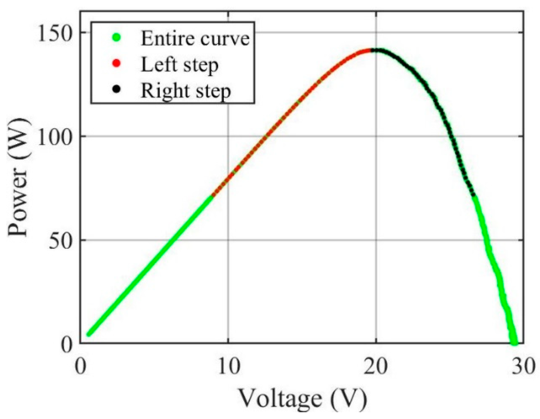
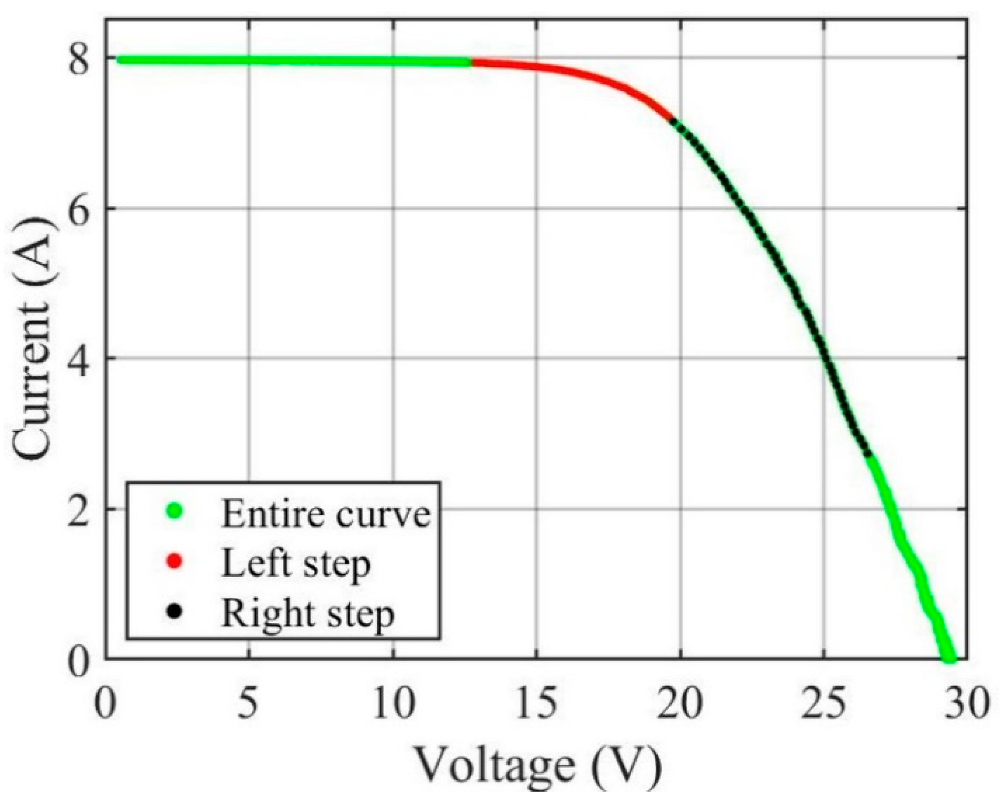
The present work provides a systematic analysis of how limiting the PV module IU curves to the vicinity of the MPP affects the fitting accuracy of the single-diode model. Two IU curve cutting approaches were examined, one of which has not been earlier systematically studied in the existing literature. In addition, the present paper is the first study to provide statistically reliable results; the experimental data of 2400 successive IU curves were subjected to a detailed analysis. The used IU curves were measured under high-irradiance conditions, where the single-diode model is known to work best.
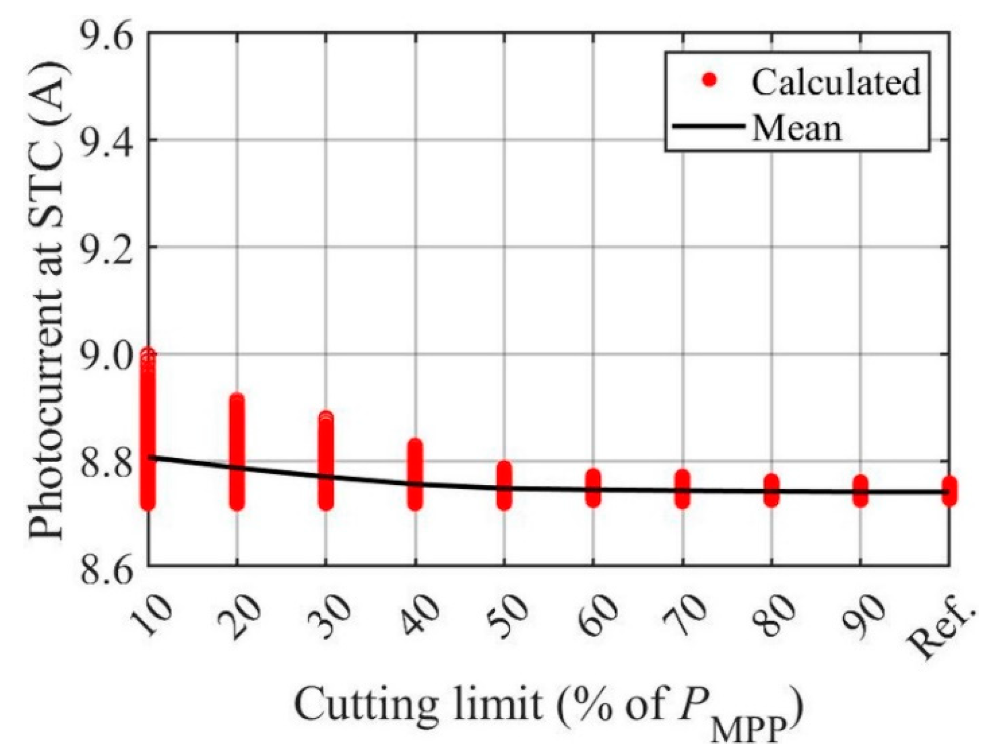
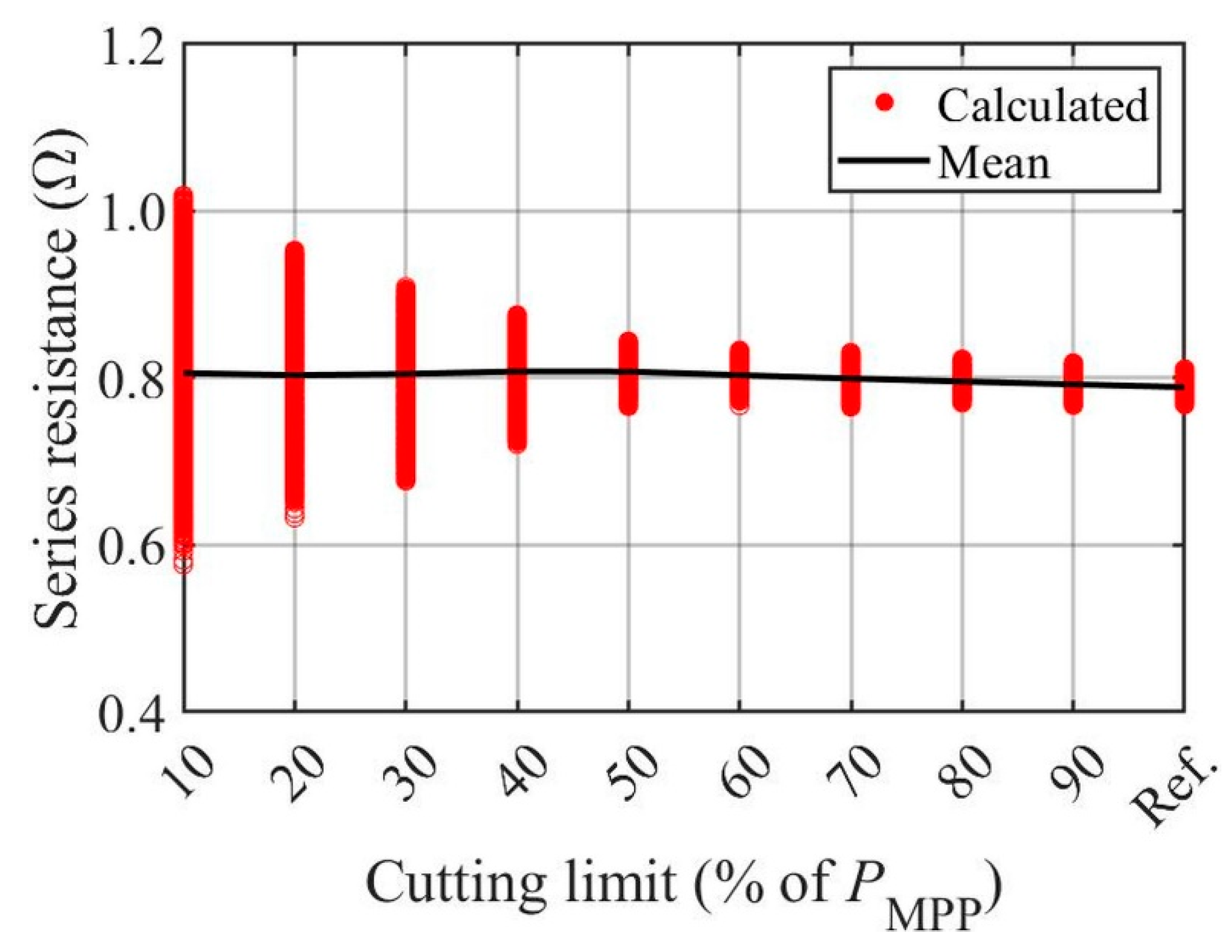
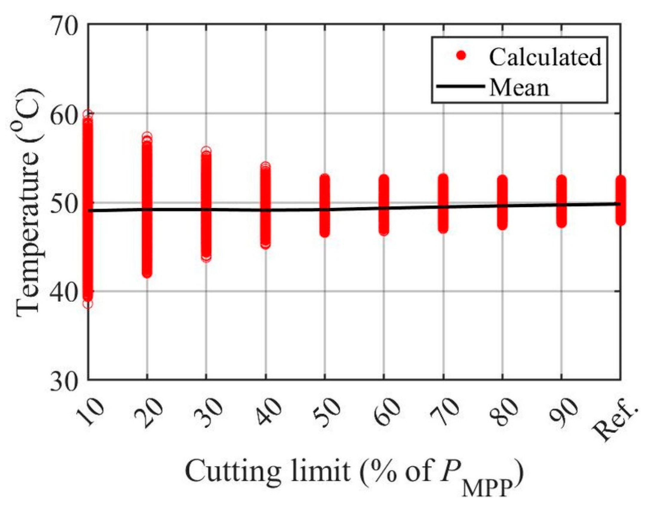
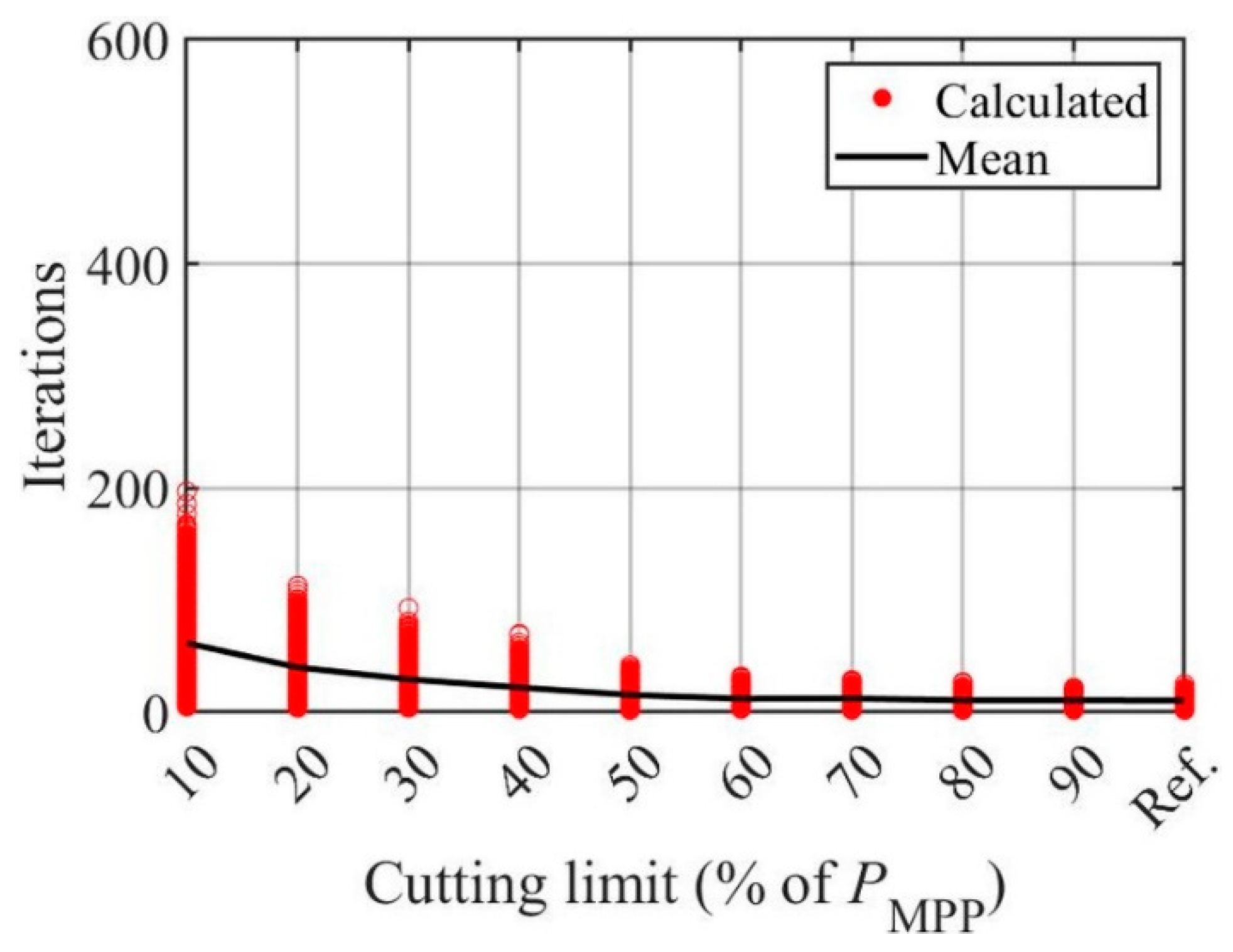
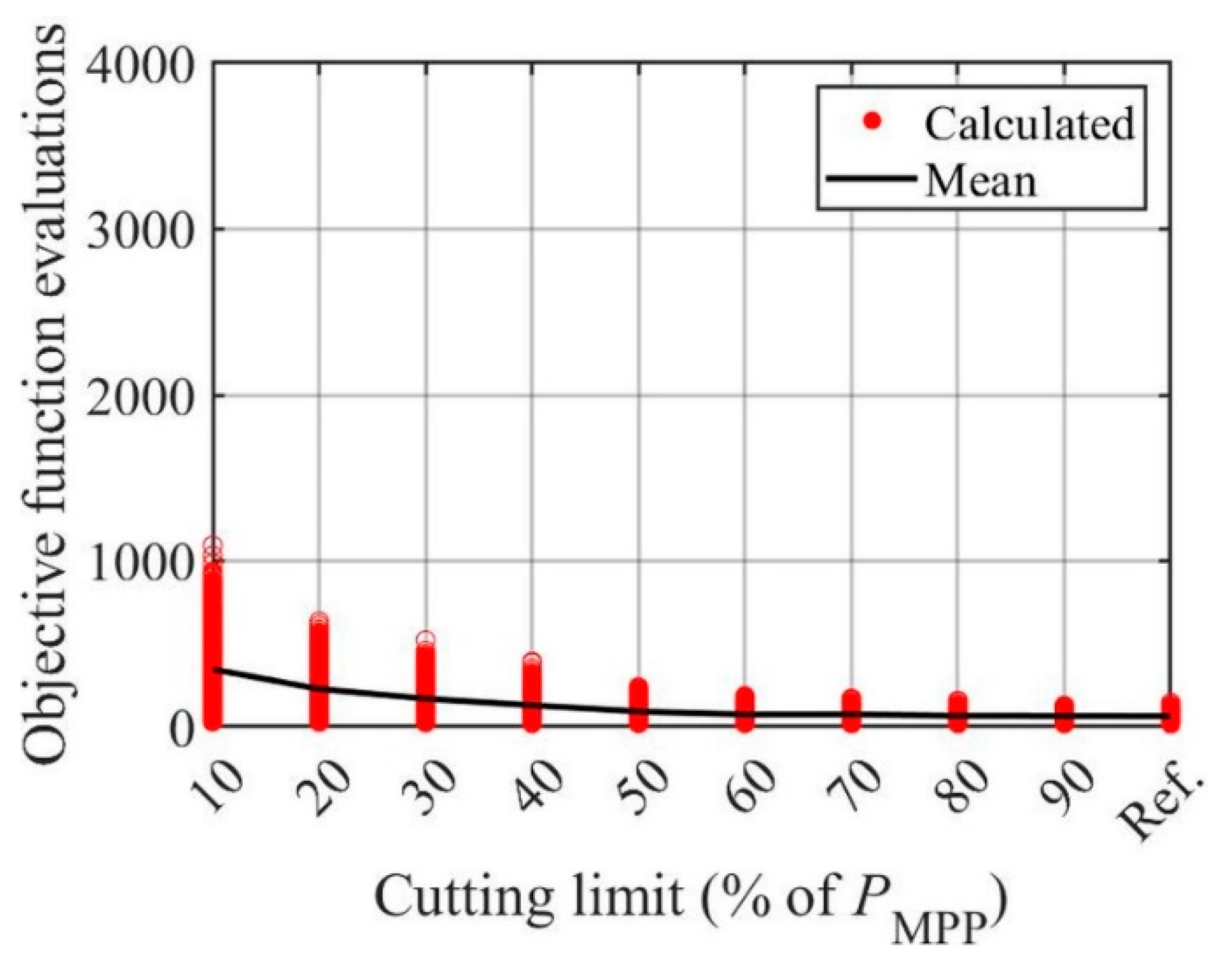
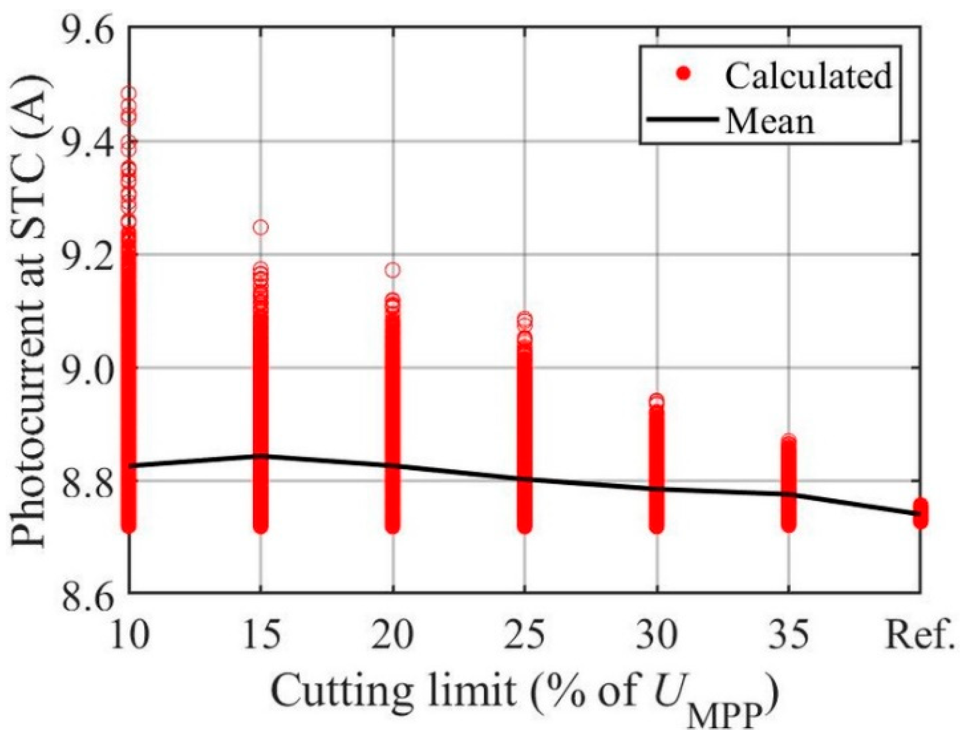
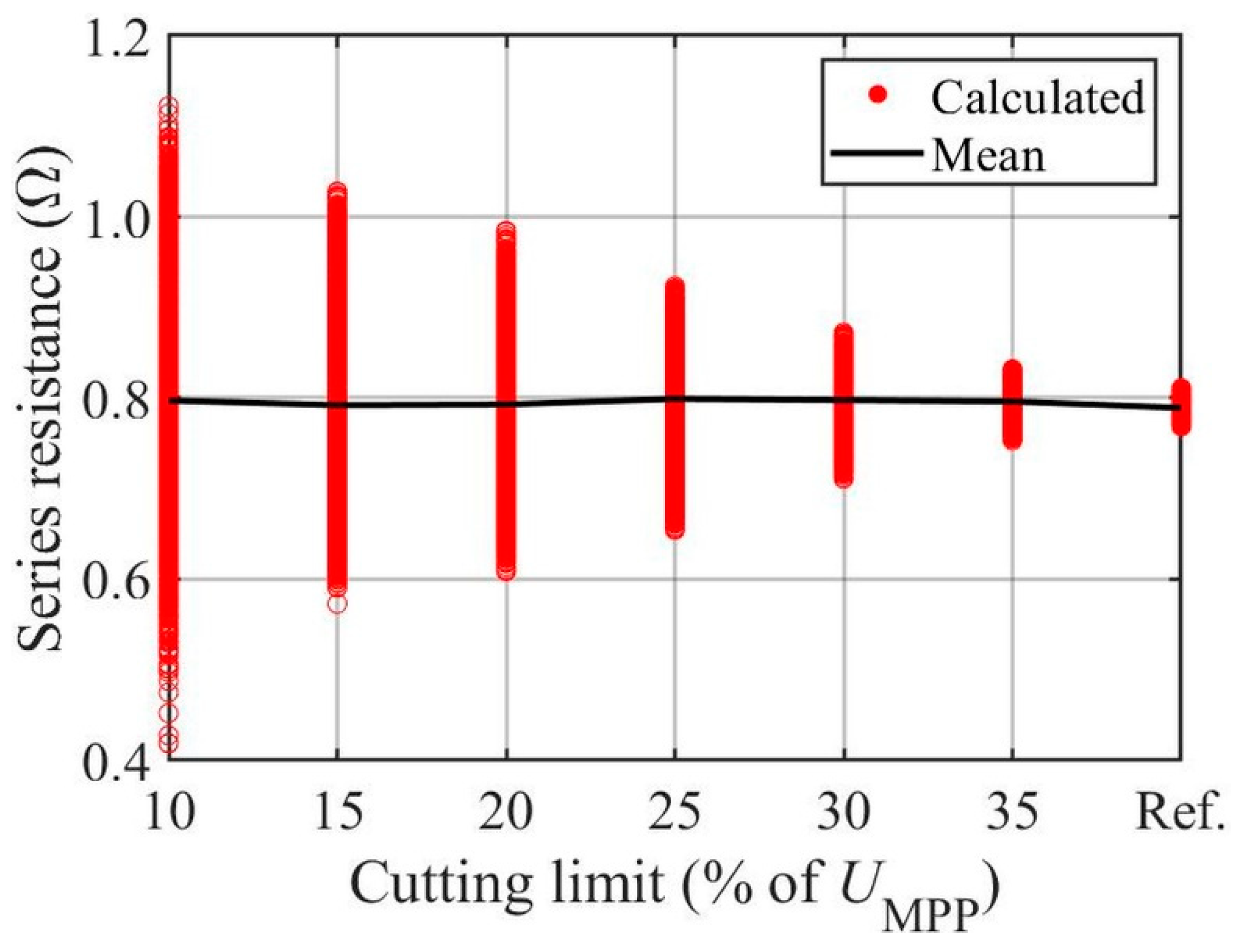
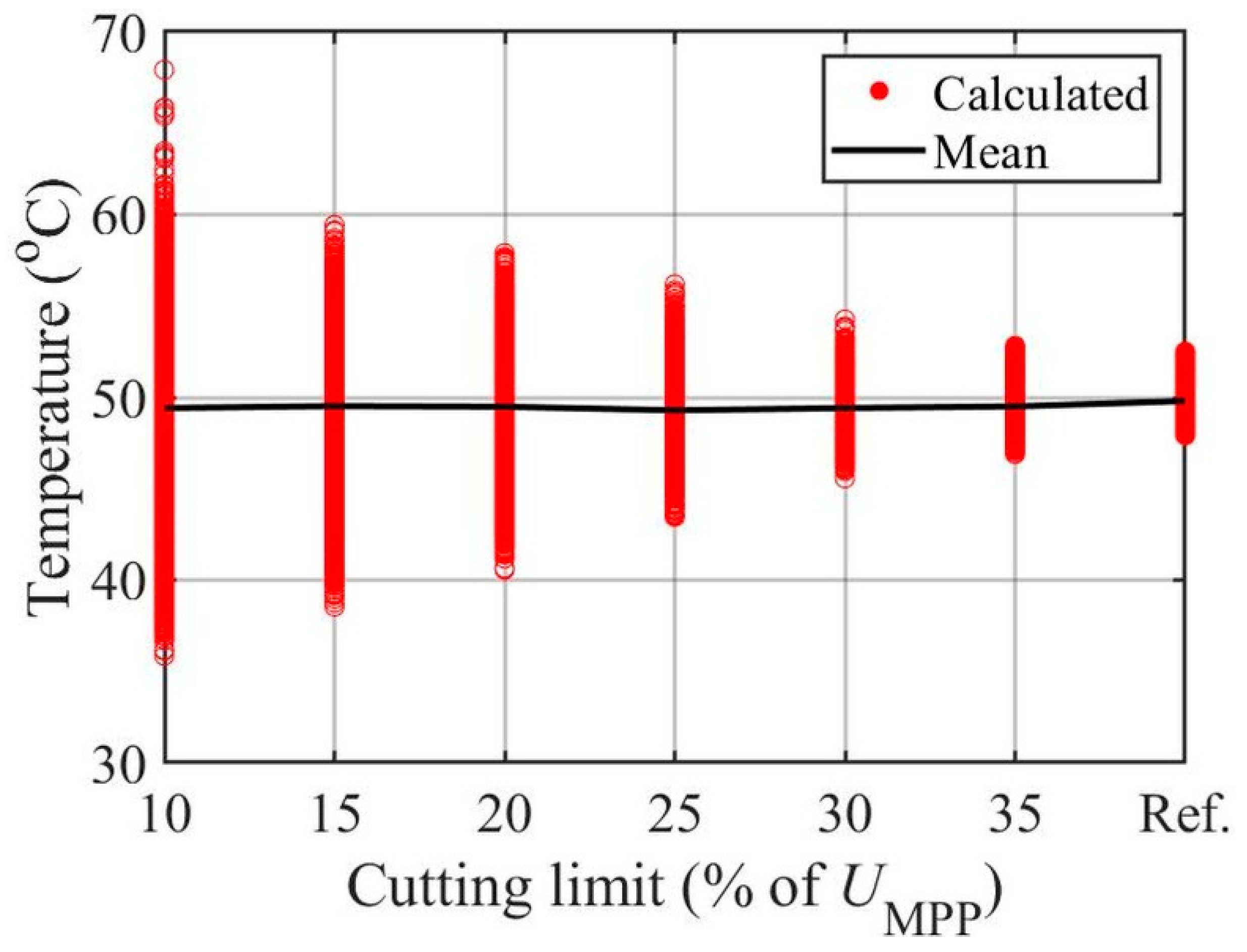
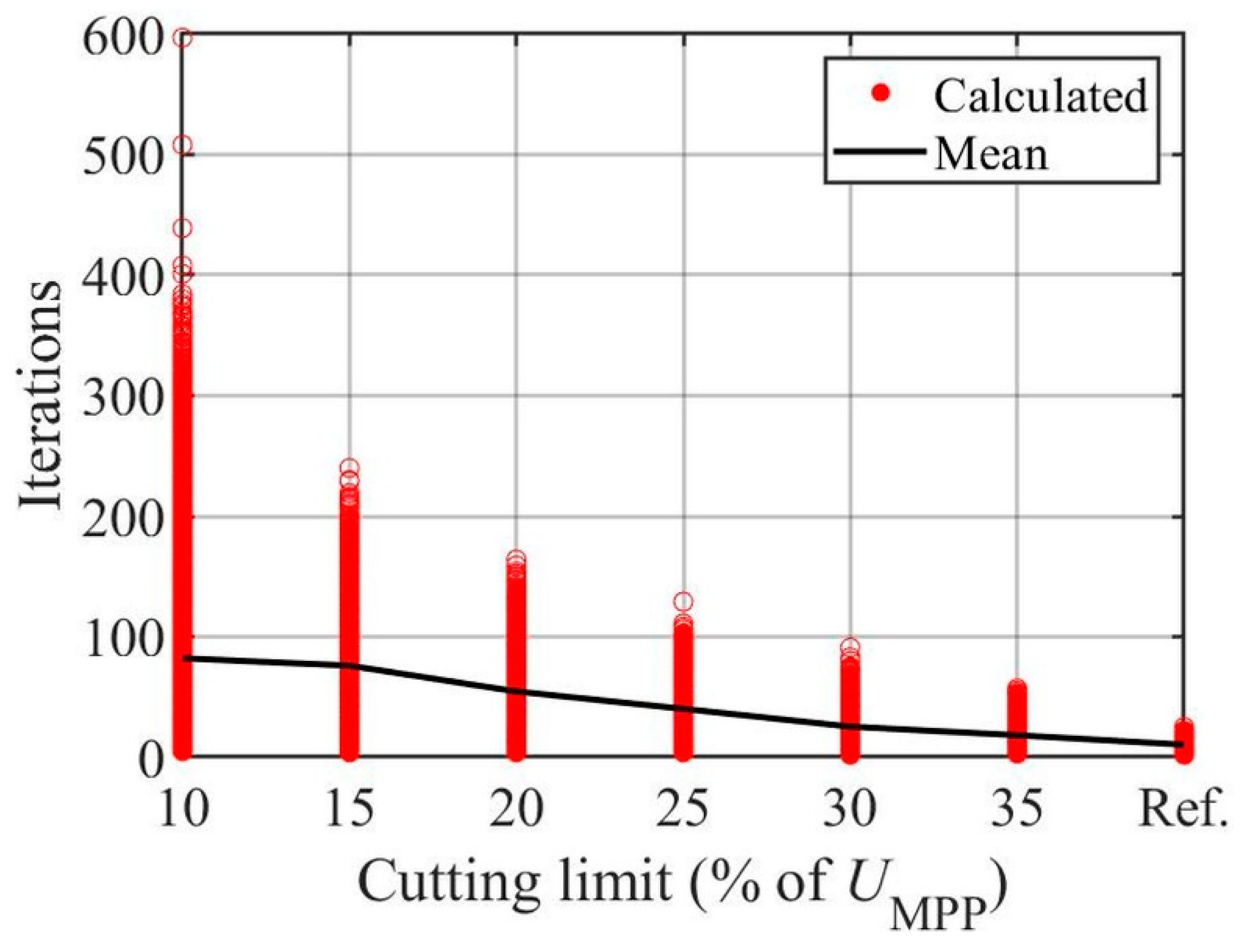
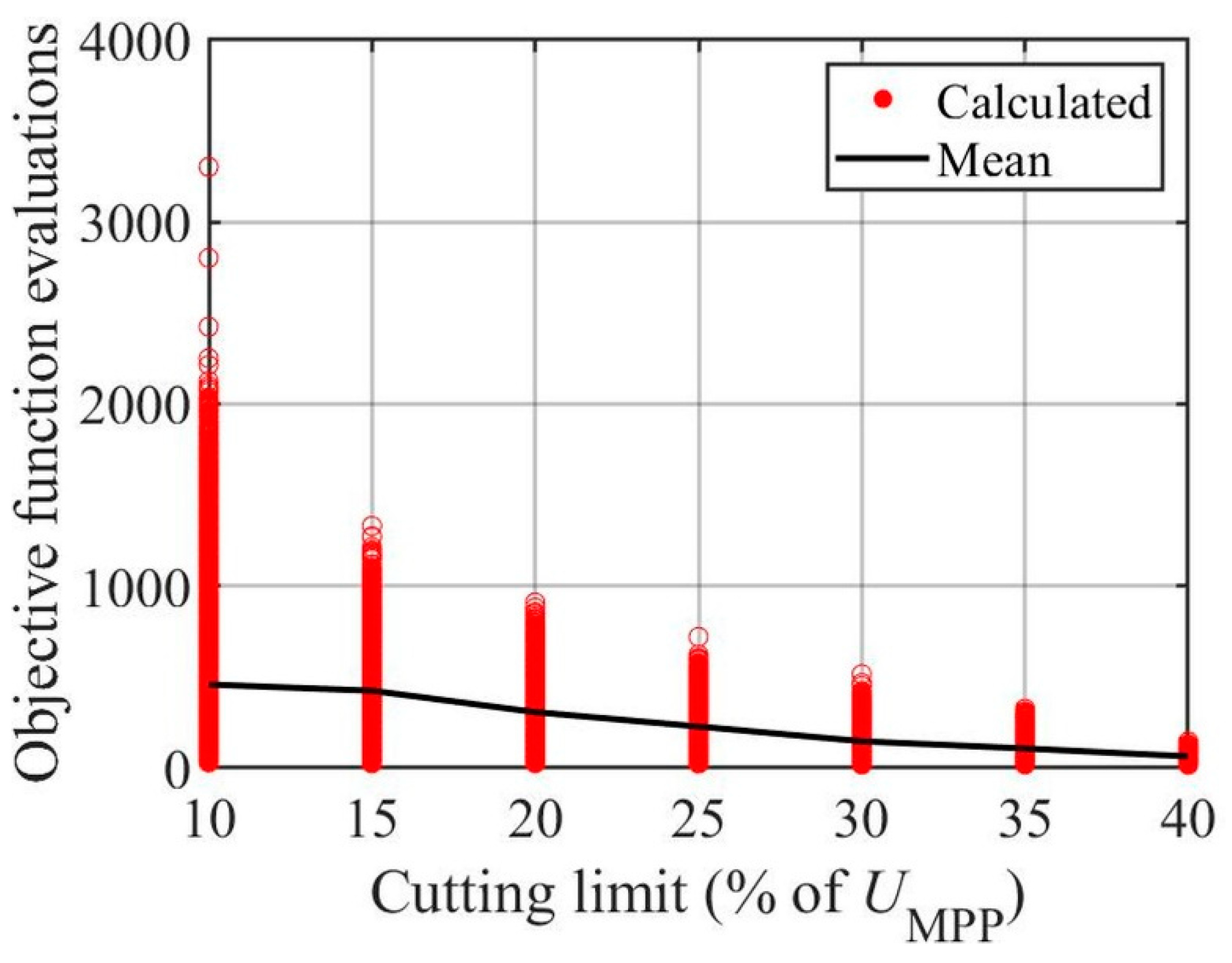
The partial IU curves were constructed step by step from complete curves to curves in the close vicinity of the MPP by setting measurement limits based on either MPP power or MPP voltage symmetrically for both sides of the MPP. The latter method was analysed for the first time in the present paper. The effect of the choice of measurement limits around the MPP was investigated for the most practical output parameters of the used single-diode model fitting procedure—photocurrent, series resistance, and temperature—from a condition monitoring point of view. The other parameters, including saturation current and shunt resistance, were omitted from this paper due to their minor significance in the condition monitoring of PV systems. It was shown that the measurement limits based on the MPP power provided more stable fitting results than the limits based on the MPP voltage. Overall, a 50% limit based on the MPP power proved to be a viable alternative for measuring partial IU curves to accurately fit a single-diode model. In contrast, the IU curves measured in very close proximity to the MPP were not sufficient for reliable aging diagnosis.
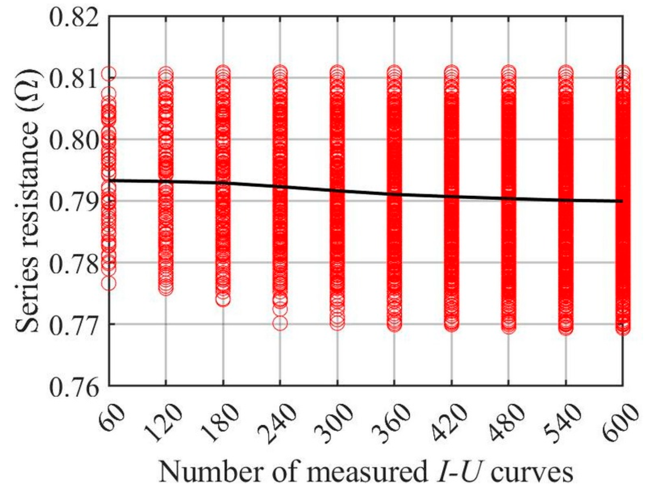
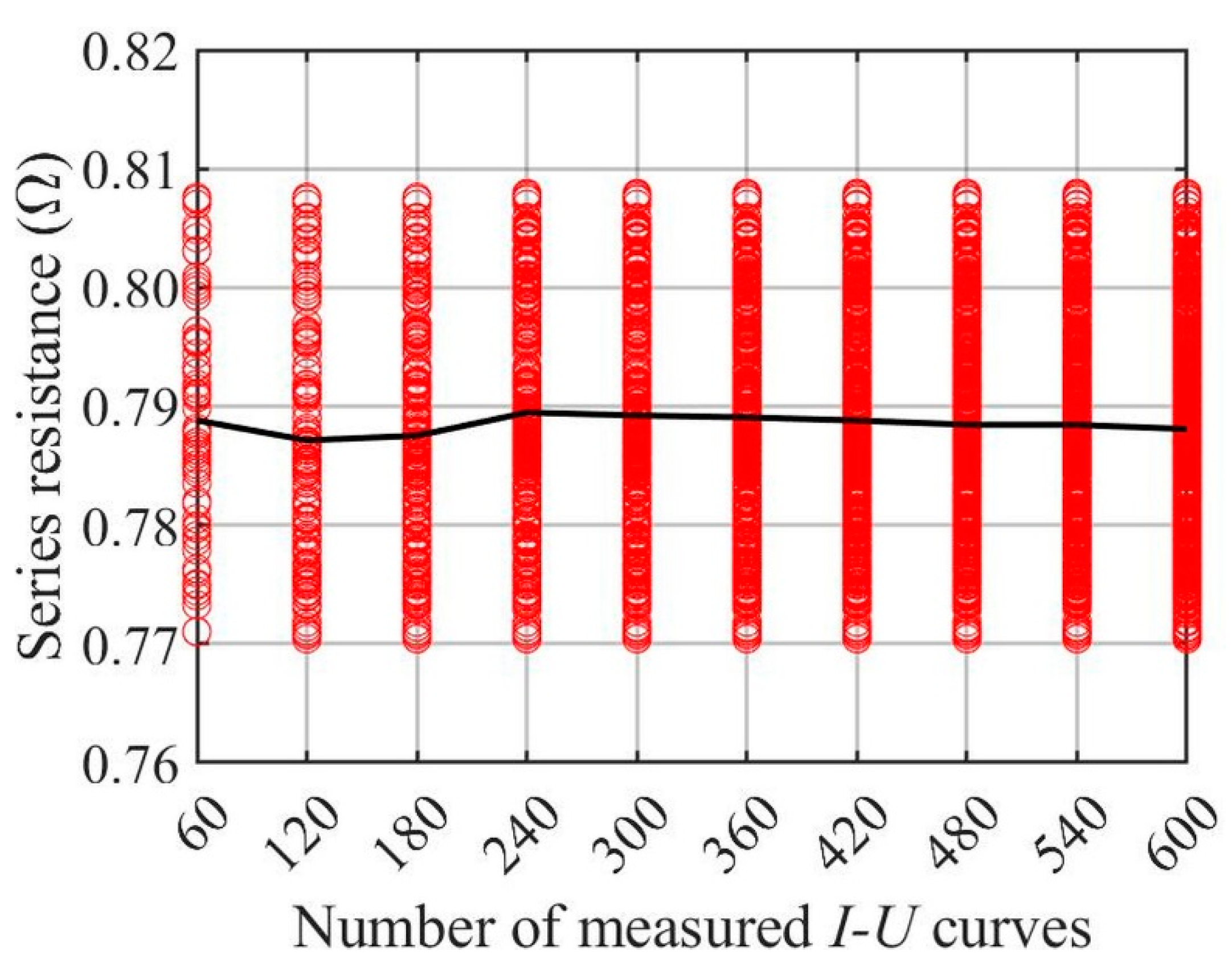
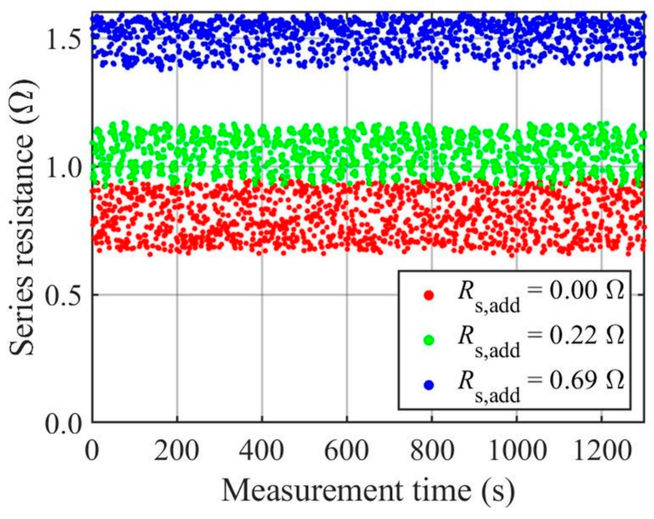
Among the single-diode model parameters, series resistance is the most important in aging detection, being also in the focus of the present paper. It was investigated how many complete IU curves are needed for reliable series resistance analysis. According to the findings, few hundred successive IU curves are sufficient. It was also found that the partial measurement of the IU curve is sufficient for series resistance analyses, as long as the open-circuit slope of the IU curve and the MPP curvature are reasonably covered. To emulate the aging of PV modules, two different-sized series resistors were still connected in series with the used PV module. The present work constitutes a strong theoretical foundation for further analyses and practical application development. In summary, the developed theoretical approach and fitting procedure, as well as the results obtained, can be used as a starting point for the development of online condition monitoring methods for PV systems.

Author Contributions

Conceptualization, H.K., K.L. and S.V.; Methodology, H.K. and K.L.; Formal analysis, H.K.; Investigation, H.K.; Data curation, K.L.; Writing—original draft, H.K.; Writing—review & editing, K.L. and S.V.; Supervision, S.V. All authors have read and agreed to the published version of the manuscript.

Funding

This research and the APC were funded by Business Finland.

Data Availability Statement

The data presented in this study are available on request from the corresponding author. The data are not publicly available due to its large amount.

Acknowledgments

The research presented in this paper was conducted as part of a project funded by Business Finland.

Conflicts of Interest

The authors declare no conflict of interest.

References

  1. Bastidas-Rodriguez, J.D.; Franco, E.; Petrone, G.; Ramos-Paja, C.A.; Spagnuolo, G. Quantification of photovoltaic module degradation using model based indicators. Math. Comput. Simul. 2017, 131, 101–113. [Google Scholar] [CrossRef]
  2. Sera, D.; Mathe, L.; Kerekes, T.; Teodorescu, R. A low-disturbance diagnostic function integrated in the PV array’s MPPT algorithm. IEEE Ind. Electron. Soc. 2011, 2456–2460. [Google Scholar] [CrossRef]
  3. Lappalainen, K.; Manganiello, P.; Piliougine, M.; Spagnuolo, G.; Valkealahti, S. Virtual Sensing of Photovoltaic Module Operating Parameters. IEEE J. Photovolt. 2020, 10, 852–862. [Google Scholar] [CrossRef]
  4. Hachana, O.; Hemsas, K.E.; Tina, G.M. Comparison of different metaheuristic algorithms for parameter identification of photovoltaic cell/module. J. Renew. Sust. Energy 2013, 5, 053122. [Google Scholar] [CrossRef]
  5. Cárdenas, A.A.; Carrasco, M.; Mancilla-David, F.; Street, A.; Cárdenas, R. Experimental Parameter Extraction in the Single-Diode Photovoltaic Model via a Reduced-Space Search. IEEE Trans. Ind. Electron. 2017, 64, 1468–1476. [Google Scholar] [CrossRef]
  6. Panchal, A.K. A per-unit-single-diode-model parameter extraction algorithm: A high-quality solution without reduced-dimensions search. Sol. Energy 2020, 207, 1070–1077. [Google Scholar] [CrossRef]
  7. Garrigós, A.; Blanes, J.M.; Carrasco, J.A.; Ejea, J.B. Real time estimation of photovoltaic modules characteristics and its application to maximum power point operation. Renew. Energy 2007, 32, 1059–1076. [Google Scholar] [CrossRef]
  8. Petrone, G.; Luna, M.; La Tona, G.; Di Piazza, M.C.; Spagnuolo, G. Online Identification of Photovoltaic Source Parameters by Using a Genetic Algorithm. Appl. Sci. 2018, 8, 9. [Google Scholar] [CrossRef] [Green Version]
  9. Blanes, J.M.; Toledo, F.J.; Montero, S.; Garrigós, A. In-Site Real-Time Photovoltaic I-V Curves and Maximum Power Point Estimator. IEEE Trans. Power Electron. 2012, 28, 1234–1240. [Google Scholar] [CrossRef]
  10. Toledo, F.J.; Blanes, J.M.; Garrigós, A.; Martinez, J.A. Analytical resolution of the electrical four-parameters model of a photovoltaic module using small perturbation around the operating point. Renew. Energy 2012, 43, 83–89. [Google Scholar] [CrossRef]
  11. Tay, S.; Lim, I.; Ye, Z.; Yang, D.; Garrigós, A. PV Parameter Identification using Reduced I-V Data. In Proceedings of the IECON 2017–43rd Annual Conference of the IEEE Industrial Electronics Society, Beijing, China, 29 October–1 November 2017; pp. 2653–2657. [Google Scholar] [CrossRef] [Green Version]
  12. Toledo, F.J.; Blanes, J.M. Analytical and quasi-explicit four arbitrary point method for extraction of solar cell single-diode model parameters. Renew. Energy 2016, 92, 346–356. [Google Scholar] [CrossRef]
  13. Lappalainen, K.; Piliougine, M.; Spagnuolo, G. Experimental comparison between various fitting approaches based on RMSE minimization for photovoltaic module parametric identification. Energy Convers. Manag. 2022, 258, 115526. [Google Scholar] [CrossRef]
  14. Kalliojärvi-Viljakainen, H.; Lappalainen, K.; Valkealahti, S. Preprocessing of PV Panel Measured Current-Voltage Characteristics before Curve Fitting. In Proceedings of the 2020 47th IEEE Photovoltaic Specialists Conference (PVSC), Virtual, 15 June–21 August 2020; pp. 117–123. [Google Scholar] [CrossRef]
  15. Petrone, G.; Ramos-Paja, C.A.; Spagnuolo, G. Photovoltaic Sources Modeling; John Wiley & Sons: Hoboken, NJ, USA, 2017. [Google Scholar]
  16. Kalliojärvi-Viljakainen, H.; Lappalainen, K.; Valkealahti, S. A novel procedure for identifying the parameters of the single-diode model and the operating conditions of a photovoltaic module from measured current–voltage curves. Energy Rep. 2022, 8, 4633–4640. [Google Scholar] [CrossRef]
  17. Kratochvil, J.A.; Boyson, W.E.; King, D.L. Photovoltaic array performance model. Sandia Natl. Lab. 2004, 20, 2004–3535. [Google Scholar] [CrossRef] [Green Version]
  18. De Soto, W.; Klein, S.A.; Beckman, W.A. Improvement and validation of a model for photovoltaic array performance. Sol. Energy 2006, 80, 78–88. [Google Scholar] [CrossRef]
  19. Villalva, M.G.; Gazoli, J.R.; Filho, E.R. Comprehensive approach for modeling and simulation of photovoltaic arrays. IEEE Trans. Power Electron. 2009, 24, 1198–1208. [Google Scholar] [CrossRef]
  20. Schroder, D.K. Semiconductor Material and Device Characterization; John Wiley & Sons: Hoboken, NJ, USA, 1998. [Google Scholar]
  21. Torres Lobera, D.; Mäki, A.; Huusari, J.; Lappalainen, K.; Suntio, T.; Valkealahti, S. Operation of TUT Solar PV Power Station Research Plant under Partial Shading Caused by Snow and Buildings. Int. J. Photoenergy 2013, 63, 837310. [Google Scholar] [CrossRef]
  22. Wolf, P.; Benda, V. Identification of PV solar cells and modules parameters by combining statistical and analytical methods. Sol. Energy 2013, 93, 153–157. [Google Scholar] [CrossRef]
  23. Moballegh, S.; Jiang, J. Modeling, prediction, and experimental validations of power peaks of PV arrays under partial shading conditions. IEEE Trans. Sust. Energy 2014, 5, 293–300. [Google Scholar] [CrossRef]
  24. Orozco-Gutierrez, M.L.; Spagnuolo, G.; Ramirez-Scarpetta, J.M.; Petrone, G.; Ramos-Paja, C.A. Optimized Configuration of Mismatched Photovoltaic Arrays. IEEE J. Photovolt. 2016, 6, 1210–1220. [Google Scholar] [CrossRef]
Figure 1. Measured IU curve jointly with 50 representative points.
Energies 15 09079 g001
Figure 2. Measured PU curve (green) jointly with cutting limits of 50% of PMPP on the left (red) and on the right (black) side of the MPP.
Energies 15 09079 g002
Figure 3. Measured IU curve (green) jointly with cutting limits of 35% of UMPP on the left (red) and on the right (black) side of the MPP.
Energies 15 09079 g003
Figure 4. The operating irradiance obtained from the fits to the entire IU curves with 100 representative points jointly with the measured irradiance during the 40 min measurement period.
Energies 15 09079 g004
Figure 5. The operating temperature obtained from the fits to the entire IU curves with 100 representative points jointly with the measured PV module backplate temperature during the 40 min measurement period.
Energies 15 09079 g005
Figure 6. Fitted photocurrent values during the 40 min measurement period converted to STCs as a function of the cutting limit based on MPP power.
Energies 15 09079 g006
Figure 7. Fitted series resistance values during the 40 min measurement period obtained by fitting the single-diode model to the entire IU curves with 100 representative points.
Energies 15 09079 g007
Figure 8. Fitted series resistance values during the 40 min measurement period as a function of the cutting limit based on MPP power.
Energies 15 09079 g008
Figure 9. Fitted temperature values during the 40 min measurement period as a function of the cutting limit based on MPP power.
Energies 15 09079 g009
Figure 10. Iterations needed for fitting during the 40 min measurement period as a function of the cutting limit based on MPP power.
Energies 15 09079 g010
Figure 11. Objective function evaluations needed for fitting during the 40 min measurement period as a function of the cutting limit based on MPP power.
Energies 15 09079 g011
Figure 12. Fitted photocurrent values converted to STCs during the 40 min measurement period as a function of the cutting limit based on the MPP voltage.
Energies 15 09079 g012
Figure 13. Fitted series resistance values during the 40 min measurement period as a function of the cutting limit based on MPP voltage.
Energies 15 09079 g013
Figure 14. Fitted temperature values during the 40 min measurement period as a function of the cutting limit based on MPP voltage.
Energies 15 09079 g014
Figure 15. Number of iterations needed for fitting during the 40 min measurement period as a function of the cutting limit based on MPP voltage.
Energies 15 09079 g015
Figure 16. Number of objective function evaluations needed for fitting during the 40 min measurement period as a function of the cutting limit based on MPP voltage.
Energies 15 09079 g016
Figure 17. Fitted series resistance values (fitted to the entire IU curves with 100 representative points) and their mean value as a function of the measurement period length starting from the curve at 1 s.
Energies 15 09079 g017
Figure 18. Fitted series resistance values (fitted to the entire IU curves with 100 representative points) and their mean value as a function of the measurement period length starting from the curve at 1201 s.
Energies 15 09079 g018
Figure 19. Fitted series resistance values using additional series resistors as a function of measurement time for the entire IU curves.
Energies 15 09079 g019
Figure 20. Fitted series resistance values using additional series resistors as a function of measurement time when using the cutting limit of 50% based on MPP power for IU curves.
Energies 15 09079 g020
Figure 21. Fitted series resistance values using additional series resistors as a function of measurement time when using the cutting limit of 20% based on MPP power for IU curves.
Energies 15 09079 g021
Table 1. The electrical characteristics of the used PV module under STCs.
ParameterValue
ISC, STC8.72 A
IMPP, STC7.94 A
UOC, STC32.8 V
UMPP, STC22.9 V
KU–0.124 V/K
KI0.0047 A/K
Rs, STC0.768 Ω
Rh, STC354 Ω
A1.10
Ns54
Table 2. Statistical quantities of the fitted series resistance values for different cutting limits based on MPP power during the 40 min measurement period.
Cutting Limit (% of PMPP)Mean (Ω)Standard Deviation (Ω)
Entire curve0.78920.0098
900.79250.0126
800.79600.0132
700.79950.0156
600.80360.0150
500.80790.0169
400.80810.0367
300.80500.0620
200.80350.0841
100.80600.1055
Table 3. Statistical quantities of the fitted series resistance for different cutting limits based on MPP voltage during the 40 min measurement period.
Cutting Limit (% of UMPP)Mean (Ω)Standard Deviation (Ω)
Entire curve0.78920.0098
350.79620.0173
300.79790.0303
250.79920.0667
200.79290.0969
150.79220.1133
100.79730.1247
Table 4. Statistics of the fitted series resistance values fitted to entire IU curves for measurement times of 1–600 s and 1201–1800 s.
1–600 s1201–1800 s
Number of CurvesMean (Ω)Standard Deviation (Ω)Mean (Ω)Standard Deviation (Ω)
600.79330.00850.78880.0102
1200.79320.00930.78710.0105
1800.79290.00950.78750.0100
2400.79230.00960.78950.0101
3000.79160.00970.78920.0099
3600.79110.00980.78910.0096
4200.79070.00990.78880.0094
4800.79040.00980.78840.0091
5400.79010.00990.78840.0091
6000.79000.01000.78810.0091
Table 5. Statistical quantities for series resistances identified from 1300 consecutive IU curves using the entirely measured IU curves (cutting limit of 100%) and partial IU curves with the cutting limits of 50% and 20% of MPP power for fitting.
Rs, add (Ω)Cutting Limit (%)Mean (Ω)Standard Deviation (Ω)
0.001000.78940.0101
500.80750.0166
200.80400.0841
0.221001.04010.0079
501.05680.0111
201.05960.0690
0.691001.50770.0080
501.51580.0127
201.50860.0580
Table 6. Difference in mean Rs values obtained from 1300 successive IU curves between aged and non-aged PV modules using entire IU curves or partial IU curves with the cutting limits of 50% and 20% of PMPP.
Rs, add (Ω)Cutting Limit of 100%Cutting Limit of 50%Cutting Limit of 20%
0.220.25070.24930.2556
0.690.71830.70830.7045
Publisher’s Note: MDPI stays neutral with regard to jurisdictional claims in published maps and institutional affiliations.

