Design and Robust Performance Analysis of Low-Order Approximation of Fractional PID Controller Based on an IABC Algorithm for an Automatic Voltage Regulator System

Abstract

In this paper, a low-order approximation (LOA) of fractional order PID (FOPID) for an automatic voltage regulator (AVR) based on the modified artificial bee colony (ABC) is proposed. The improved artificial bee colony (IABC) high-order approximation (HOA)-based fractional order PID (IABC/HOA-FOPID) controller, which is distinguished by a significant order approximation and by an integer order transfer function, requires the use of a large number of parameters. To improve the AVR system’s performance in terms of transient and frequency response analysis, the memory capacity of the IABC/HOA-FOPID controller was lowered so that it could fit better in the corrective loop. The new robust controller is named the improved artificial bee colony (IABC) low-order approximation (LOA)-based fractional order PID (IABC/LOA-FOPID). The performance of the proposed IABC/LOA-FOPID controller was compared not only to the original ABC algorithm-tuned PID controller, but also to other controllers tuned by state-of-the-art meta-heuristic algorithms such as the improved whale optimization algorithm (IWOA), particle swarm optimization (PSO), cuckoo search (CS), many optimizing liaisons (MOL), genetic algorithm (GA), local unimodal sampling (LUS), and the tree seed algorithm (TSA). Step response, root locus, frequency response, robustness test, and disturbance rejection abilities are all compared. The simulation results and comparisons with the proposed IABC/LOA-FOPID controller and other existing controllers clearly show that the proposed IABC/LOA-FOPID controller outperforms the optimal PID controllers found by other algorithms in all the aforementioned performance tests.

1. Introduction

In power systems, the automated voltage regulator (AVR) is employed to maintain the terminal voltage of a synchronous generator at a suitable level. The AVR system regulates the constancy of the terminal voltage by adjusting the generator’s exciter voltage [1,2]. In power system applications, maintaining a consistent input voltage has always been a difficult problem. When there is a sudden shift in load for power supply requirements, the AVR system is employed to stabilize the voltage value.

The AVR system is now receiving a lot of attention in the industry for keeping the synchronous generator’s terminal voltage constant under all situations. Classical integer order proportional-integral-derivative (IOPID) [3,4,5], proportional-integral-derivative acceleration (PIDA) [6], fractional order PID (FOPID) [7,8,9], PID plus second-order derivative (PIDD2) controller [10], modified neural network (MNN) [11], genetic algorithm (GA) [12], interval type-2 fuzzy logic (IT2FL) [13], and a differential evolution—artificial electric field algorithm (DE-AEFA) [14].

Likewise, the objective function can also be of any type such as integral of time multiplied square error (ITSE) [15], integral of time multiplied absolute error (ITAE) [16], integral absolute error (IAE) [17] and integral square error (ISE) [18].

However, even for the same controllers, several optimization methods are available. For example, artificial bee colony (ABC) [15], stochastic fractal search [19], whale optimization algorithm (WOA) [20], improved whale optimization algorithm (IWOA) [21], sine-cosine algorithm (SCA) [22], tree seed algorithm (TSA) [23], particle swarm optimization (PSO) [24], improved kidney-inspired algorithm (IKIA) [25], cuckoo search (CS) [26], genetic algorithm [12,27], many optimizing liaisons (MOL) [28], grey wolf optimization (GWO) [18], crow search algorithm (CSA) [29], water wave optimization (WWO) [30], local unimodal sampling (LUS) [31], water cycle algorithm (WCA) [32], and ant colony optimization (ACO) [33], are optimization algorithms that have been proposed to tune the controller parameters of an AVR system. In refs. [14,34], the authors investigated the combined analysis of load frequency control (LFC) and automatic voltage regulation (AVR), where a differential evolution—artificial electric field algorithm—is presented and is applied to the combined LFC-AVR model. Further examples of the intelligent strategies for achieving optimal parameters in various systems can be found in [35,36,37,38].

Using fractional calculus, it is possible to improve the performance of the PID controller in AVR systems. The FOPID controller (FOPID) is a type of classical PID controller that employs fractions instead of integers in order of derivation and integration. Furthermore, as compared to the integer order PID controller, FOPID provides a better transient response while also being more robust and stable [39,40,41,42,43,44,45]. Because of the previously indicated benefits of the FOPID, this research focuses on this form of controller.

In this paper a low-order approximation (LOA) of fractional order PID (FOPID) based on the artificial bee colony (ABC) has been proposed. The IABC/FOPID controller approximation, which is distinguished by a transfer function of integer order and a long memory (or high order approximation (HOA)), named IABC/HOA-FOPID, and requires a lot of parameters to be used. To enhance the performance of the AVR system in terms of transient and frequency responses analysis, the complete IABC/HOA-FOPID controller’s memory capacity was reduced so that it could fit better in the corrective loop, the new robust controller is named IABC/LOA-FOPID.

The following list summarizes this paper’s originality contribution:

-

For the first time, the low-order approximation of a FOPID controller based on the ABC algorithm (named IABC/LOA-FOPID) is used.

-

In terms of transient response performance, the proposed IABC/LOA-FOPID controller was thoroughly compared to various strategies in the literature, such as IWOA-PID [21], PSO-PID [12], ABC-PID [15], CS-PID [26], MOL-PID [28], GA-PID [12], LUS-PID [31], and TSA [23]. The findings of the research clearly show that the LOA-FOPID controller tuned by IABC is better.

-

To investigate the system’s behavior, several robustness tests are specifically studied. All along the experiments, the LOA-FOPID regulator optimized by ABC outperforms the classical or fractional PID controller, whose parameters have been optimized by the other methods that have been researched in the literature.

This paper is organized as follows: Section 2 provides a brief overview of the AVR system’s composition, the fundamentals of fractional calculus, and the stability of fractional order systems. Section 3 provides a thorough explanation and mathematical formulation of the proposed IABC/LOA-FOPID controller. The simulation results are displayed in Section 4 of this study. Section 5 summarizes the study’s overall findings.

2. Materials and Methods

2.1. AVR System Description and Modeling

The basic role of an AVR system is to keep the generator’s terminal voltage constant via the excitation system. A basic AVR system consists of four major components: an amplifier, an exciter, a generator, and a sensor. These components are represented by transfer functions [9,12,15,46] and modeled in the MATLAB/Simulink environment to study the dynamic performance of an AVR. A first-order transfer function with a gain and a time constant is used to represent each component of the AVR system.

Table 1. Main components of AVR system.

Component of AVR System	Transfer Function	Gain Range	Time Constant Range [s]
Amplifier	$G_a=\frac{K_a}{1+T_{a}s}$	$10<K_a<400$	$0.02<T_a<0.1$
Exciter	$G_e=\frac{K_e}{1+T_{e}s}$	$1<K_e<400$	$0.4<T_e<1$
Generator	$G_g=\frac{K_g}{1+T_{g}s}$	$0.7<K_g<1$	$1<T_g<2$
Sensor	$G_s=\frac{K_s}{1+T_{s}s}$	$K_s=1$	$0.001<T_s<0.06$

shows the transfer functions of the aforementioned components. The closed-loop block diagram of the AVR system without a controller is shown in Figure 1 along with the transfer functions.

To compare the results fairly, in this work, the AVR system’s parameters are K_a = 10, K_e = 1, K_g = 1, K_s = 1, T_a = 0.1, T_e = 0.4, T_g = 1 and T_s = 0.01, which are the same as in the research works [12,15,21,23,26,28,31]. The closed loop transfer function for the AVR system is found as the following equation given the model parameter values mentioned above.

$$\frac{V_{out}}{V_{ref}}=\frac{0.1s+10}{0.0004s^4+0.045s^3+0.555s^2+1.51+11}$$

(1)

Figure 2 depicts the output step voltage response of the aforementioned system, which makes it evident that it is oscillatory stable.

Table 2. Values of the AVR system’s transient response without a controller.

Controller Type	Mp [%]	ts [s]	tr [s]
AVR without controller	65.7226	6.9865	0.2607

presents the AVR system’s transient response characteristics maximum overshoot (M_p [%]), settling time (t_s [s]) and rise time (t_r [s]) in the absence of the controller.

2.2. Fractional Calculus

Fractional calculus is a non-integer order operator $a{D}_t^{\alpha }$ extension of integration and differentiation, where a and t signify the operation’s limits and denote the fractional order such that

$$a{D}_t^{\alpha }=\{\begin{array}{c}\frac{d^{\alpha }}{d{t}^{\alpha }} , R\left(\alpha \right)>0\\ 1 , R\left(\alpha \right)=0\\ \underset{a}{\overset{t}{{\displaystyle \int }}}{\left(d\tau \right)}^{-\alpha },R\left(\alpha \right)<0 \end{array}$$

(2)

where it is commonly believed that $\alpha \in ℝ$, although it might alternatively be a complex number. The fractional differintegral has several definitions. A typical definition is the Riemann-Liouville differintegral [47].

Definition 1.

The mathematical definition of Grünwald–Letnikov is:

$$D^{\alpha }f\left(t\right)=\underset{h\to 0}{lim}{h}^{-\alpha }{{\displaystyle \sum }}_{j=0}^k{\left(-1\right)}^j\left(\begin{array}{c}\alpha \\ j\end{array}\right)f\left(kh-jh\right)$$

(3)

Here, ‘h’ is the step time and the coefficients given above can be evaluated in relation to the expression given below;

$${\omega }_j^{\left(\alpha \right)}=\left(\begin{array}{c}\alpha \\ j\end{array}\right)=\frac{\mathsf{Ӷ}\left(\alpha +1\right)}{\mathsf{Ӷ}\left(j+1\right)\mathsf{Ӷ}\left(\alpha -j+1\right)}$$

(4)

Definition 2.

Mathematically, the Riemann-Liouville definition is:

$$f\left(t\right)=\frac{d^n}{d{t}^n}\underset{0}{\overset{t}{{\displaystyle \int }}}\frac{f\left(\tau \right)}{{\left(t-\tau \right)}^{\alpha -n+1}}d\tau$$

(5)

The Oustaloup methodology performs by approximating the function from as:

$$G_f\left(s\right)=S^{\alpha } , \alpha \in R^{+}$$

(6)

Taking the rational function into consideration [48,49]:

$$G_f\left(s\right)=K{\displaystyle \prod }_{k=1}^N\frac{s+w_k^{\prime }}{s+w_k}$$

(7)

However, gain, zeros, and poles can be calculated as follows:

$$K=w_h^{\gamma },w_k=w_b.w_u^{\left(2k-1+\gamma \right)/N},w_k^{\prime }=w_b.w_u^{\left(2k-1-\gamma \right)/N}$$

where w_u represents the unity gain in frequency and the central frequency in a geometrically distributed frequency band. Let,$w_u=\sqrt{w_h{w}_b}$, where w_h represents the upper frequencies while w_b represents the lower frequencies, γ is the derivative order and N is the filter.

2.3. Stability of Fractional Order Systems

When developing a control system, stability is a fundamental and critical condition. In integer order, a linear time-invariant (LTI) system in continuous-time is stable if all of the characteristic equation’s roots are on the left half of the ‘s’ plane.

The stability of fractional order is determined by more than simply the placements of the poles on the left half side. The fractional order determines it, which becomes progressively complicated as seen below. The characteristic equation of a general linear fractional differential equation is as follows:

$${{\displaystyle \sum }}_{i=0}^j{a}_i{s}^{{\alpha }_i}=0$$

(8)

where, α_i is rational, the characteristic equation can be rewritten as;

$${{\displaystyle \sum }}_{i=0}^n{a}_i{s}^{\frac{i}{m}}=0$$

(9)

where m is integer, α = 1/m and α_i > 0.

Figure 3a shows the stability zone of a fractional order system when 0 < α < 1, which is greater than the stability region of an integer order system. Figure 3b shows the stability zone of a fractional order system when 1 < α < 2, which is smaller than the stability region of an integer order system [50,51].

3. Fractional PID Controller Based on IABC Algorithm

3.1. ABC Algorithm

The employed bees, following bees, and scout bees are the three categories that the basic algorithm of the artificial bee colony divides the population and assigns a search to each type of artificial bee phase [52,53]. As a starting point, the initial solution (food sources) is arbitrarily generated. All solutions $X_i=\left(i=1, 2,\dots , N\right)$; $X_i={\left(x_{i1}, x_{i2}, x_{i3},\dots , x_{id}\right)}^T$ stands for the position of all food sources.

Equation (10) is used by the employed bee to conduct a random search of the feasible domain in search of food sources. The deployed bee then passes the results of the food source multiplication to the next bee, which is waiting in the hive to perform the food source search.

$$x_{ij}^{\prime }=x_{ij}+r_{ij}\left(x_{ij}-x_{kj}\right)$$

(10)

where k = 1, 2, …, N and j = 1, 2, …, d. k is a randomly selected indicator for different i. N stands for the population size, and D stands for the problem dimension, r_ij is a random number between −1 and 1.

In the following bee stage, the food source is selected by the onlooker bee based on likelihood. As can be seen from (Equation (11)) below, the probability value, prob(i), is calculated:

$$prob\left(i\right)=\frac{fit\left(i\right)}{{{\displaystyle \sum }}_{i=1}^{N}fit(i)}$$

(11)

When an onlooker makes a decision about which food source to choose, it starts searching for it, generates an updated location by (10), assesses the profitability, and then remembers the better location. fit(i) in (11) represents the fitness value of the ith food source X_i.

The scout bees reject all food sources that have previously been used to make honey during this phase, going over the permitted intake for all food sources. A bee that has been working on a food source that has been abandoned eventually develops into a scout bee. The scout will investigate a new food source at random (12).

$$x_{ij}=x_{min,j}+rand\left(0,1\right)\left(x_{max,j}-x_{min,j}\right)$$

(12)

3.2. Fractional Order PID Controller

Classical PID controllers are frequently used because of their basic design and simple implementation. The dynamic response of the AVR system can be improved by using controllers with fractional order PID (FOPID) or integer order PID (IOPID). With respect to the error signal, the PID controller executes three major control actions using proportional, integral, and derivative approaches. The PID controller transfer function is provided by:

$$G_{IOPID}\left(s\right)=K_p+\frac{K_i}{s}+K_{d}s$$

(13)

where K_p represents the proportional gain, and K_i and K_d represent the integral and derivative gains respectively.

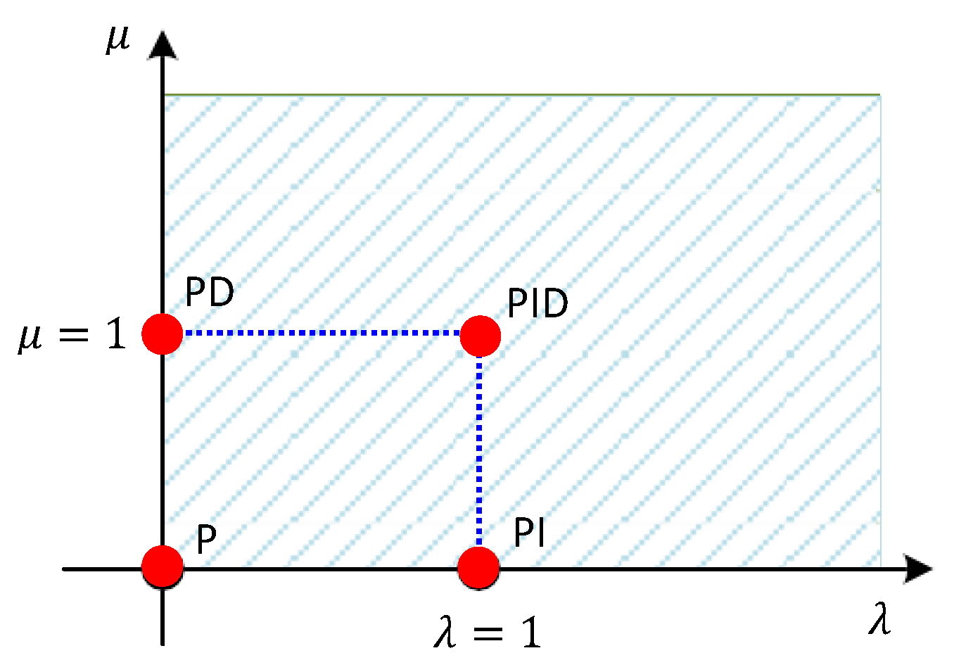
The fractional order PID controller is an extension of the traditional PID controller, offering an integration of order λ and a differentiation of order μ, where λ and μ can be any positive real integer.

$$G_{FOPID}\left(s\right)=K_p+\frac{K_i}{s^{\lambda }}+K_d{s}^{\mu }$$

(14)

where the two additional parameters are λ (fractional order integration) and μ. (fractional order differentiation).

The fractional PID controller is the most popular kind of PID controller because of its original characteristics. There are various kinds of FOPID controllers, such as PID $\left(\lambda =1, \mu =1\right),$ PI $\left(\lambda =1, \mu =0\right),$ PD $\left(\lambda =0, \mu =1\right)$, and the P controller $\left(\lambda =0, \mu =0\right)$. The graphical representation of the various PID controllers is shown in Figure 4.

3.3. Design of the FOPID Controller Using IABC

To optimize the parameters of the FOPID controller ($K_p, K_i, K_d, \lambda , \mu )$, the modified ABC algorithm presented in [52], which is based on the use of cyclic exchange neighborhood and chaos (CNC), is used. Figure 5 depicts an AVR system with an IABC-FOPID controller. A food source location represents a potential solution of the FOPID controller to be optimized, which is represented by a vector with five components,$X=\left(K_p, K_i, K_d, \lambda , \mu \right)$. Each solution’s fitness is determined by (15).

The modified ABC algorithm described in [50], which is based on the use of the cyclic exchange neighborhood and chaos (CNC), is used to optimize the parameters of the FOPID controller ($K_p, K_i, K_d, \lambda , \mu )$. An AVR system with an IABC/LOA-FOPID controller is shown in Figure 5. The FOPID controller to be optimized has a potential solution represented by a food source location, which is represented by a vector with five components, $X=\left(K_p, K_i, K_d, \lambda , \mu \right)$.

The fitness of each solution is given by (15).

$$J\left(K_P,K_I,K_D,\lambda ,\mu \right)={{\displaystyle \int }}_0^{\infty }|y{(t)}^{*}-y\left(t\right)|dt={{\displaystyle \int }}_0^{\infty }\left|e\left(t\right)\right|dt$$

(15)

where: $y\left(t\right)$ represents the output of the system, in our case is the output voltage of the generator; noted $V_{out}$. $y{\left(t\right)}^{*}$ is the reference voltage; noted $V_{ref}$.

The following are the main design steps [52].

Step 1: Start with the basic solution.

Step 2: Determine each initial solution’s fitness $x_i$.

Step 3: Set cycle to 1.

Step 4: Bees are used to produce new solutions $x_i$, and fitness is calculated, both using (16) and (15);

$$x_{ij}^{\prime }=\{\begin{array}{cc}{x}_{Nj}+r_{ij}\left(x_{ij}-x_{kj}\right),& i=1\\ x_{i-1j}+r_{ij}\left(x_{ij}-x_{kj}\right),& 2\le i\le N\end{array}$$

(16)

Step 5: Use the greedy selection to select the best one between $x_i^{\prime }$ and $x_i$.

Step 6: Using Equation (11), compute the probability values prob(i) of the solutions.

Step 7: Onlooker bees select the solution based on prob(i), then look for a neighbor to generate new solutions by (10) and calculate fitness by (15).

Step 8: Use a greedy choice to find the right and best solution.

Step 9: If a solution requires improvement, scouts should conduct a search for chaos.

Step 10: Commit the best answer so far to memory.

Step 11: Cycle = cycle + 1; if cycle is greater than the allowed number of cycles, the process is stopped; if not, move on to step 4.

Figure 5 illustrates the block design for the proposed IABC/LOA-FOPID controller used in an AVR system.

3.4. Sub-Optimal Reduction Algorithm

Figure 6 shows the error signal for model reduction, where the initial model is provided by:

$$G\left(s\right)=\frac{b_{n-1}{s}^{n-1}+\dots +b_{1}s+b_0}{s^n+a_{n-1}{s}^{n-1}+\dots +a_{1}s+a_0}$$

(17)

Our present goal is to develop a low-order approximation (LOA) integer-order model of the type in [54]:

$$G_{r/m}\left(s\right)=\frac{{\beta }_1{s}^r+\dots +{\beta }_{r}s+{\beta }_{r+1}}{s^m+{\alpha }_1{s}^{m-1}+\dots +{\alpha }_{m-1}s+{\alpha }_m}$$

(18)

An objective function to reduce the H2 norm of the reduction error signal is as follows:

$$J_r=\underset{\mathsf{\theta }}{\min }\Vert \widehat{G}\left(s\right)-G_{r/m}\left(s\right){\Vert }_2$$

(19)

With $\theta$ the parameters are to enhance such that:

$$\theta =\left[{\beta }_1,\dots ,{\beta }_r,{\alpha }_1,\dots ,{\alpha }_m\right]$$

(20)

To find the low-order approximation (LOA) model of the fractional-order model characterized by a long memory, use the following approaches [55]:

• Choose an initial simplified model ${\widehat{G}}_r^0\left(s\right)$.
• Get an error function ${\Vert \hat{G}(s)-{\hat{G}}_{r/m}(s)\Vert }_2$
• Use the Powell optimization method [55] to iterate a step to obtain a better estimation of the ${\widehat{G}}_{r/m}^1\left(s\right)$ model.
• Set ${\widehat{G}}_{r/m}^0\left(s\right) \leftarrow {\widehat{G}}_{r/m}^1\left(s\right)$, go to step 2 until an optimal LOA model ${\widehat{G}}_{\frac{r}{m}}^{*}\left(s\right)$ is obtained.

4. Results and Discussion

The algorithm’s performance in managing the AVR system specified in Equation (1) is validated by the simulations that follow. The simulations were created using the MATLAB/SIMULINK software.

Table 3. IABC-FOPID Parameters for solving optimization problems.

Parameter	Value
Population size	$40$
Maximum cycle number	$200$
$\mathrm{Lower}\mathrm{bound}\mathrm{for}\left[K_p;K_i;K_d;\lambda ;\mu \right]$	$\left[0.001;0.001;0.001;0.001;0.001\right]$
$\mathrm{Upper}\mathrm{bound}\mathrm{for}\left[K_p;K_i;K_d;\lambda ;\mu \right]$	$\left[15;10;10;2;2\right]$
Dimension for optimization problem	5

provides a list of the proposed IABC algorithm’s parameters.

Table 4. Gain parameters of the proposed controller and other compared controllers.

Controller Type	Kp	Ki	Kd	λ	μ
IABC/LOA-FOPID [Proposed]	1.9605	0.4922	0.2355	1.4331	1.5508
IWOA-PID [21]	0.8167	0.6898	0.2799	1	1
PSO-PID [12]	0.6254	0.4577	0.2187	1	1
ABC-PID [15]	0.6352	0.4235	0.2241	1	1
CS-PID [26]	0.6198	0.4165	0.2126	1	1
MOL-PID [28]	0.5857	0.4189	0.1772	1	1
GA-PID [12]	0.8851	0.7984	0.3158	1	1
LUS-PID [31]	0.6190	0.4222	0.2058	1	1
TSA [23]	1.1281	0.9567	0.5671	1	1

shows the parameters of the IABC/LOA-FOPID controller that was identified during the optimization process.

For the AVR model system given in Equation (1) with the following fractional PID parameters: $K_p=1.9605, K_i=0.4922, K_d=0.2355$, $\lambda =1.4331$ and $\mu =1.5508$, an IABC algorithm is used to build a fractional PID controller.

The IABC/FPID controller is given by:

$$G_{IABC/FOPID}\left(s\right)=1.9605+0.4922s^{-1.4331}+0.2355s^{1.5508}$$

(21)

Consequently, the Oustaloup approach with ${\omega }_b=0.1 \mathrm{rad}/\mathrm{s}$, ${\omega }_h=10 \mathrm{rad}/\mathrm{s}$ and unity feedback yields the IABC/HOA-FOPID controller’s closed loop transfer function as follows:

$$G_{C{L}_{IABC/HOA-FOPID}}\left(s\right)=\frac{\begin{array}{c}0.08371{\mathrm{s}}^{13}+10.18{\mathrm{s}}^{12}+197.6{\mathrm{s}}^{11}+1756{\mathrm{s}}^{10}+9249{\mathrm{s}}^9+\\ 3.152\mathrm{e}04{\mathrm{s}}^8+7.033\mathrm{e}04{\mathrm{s}}^7+1.016\mathrm{e}05{\mathrm{s}}^6+9.449\mathrm{e}04{\mathrm{s}}^5+\\ 5.696\mathrm{e}04{\mathrm{s}}^4+2.234\mathrm{e}04{\mathrm{s}}^3+5553{\mathrm{s}}^2+786.3\mathrm{s}+47.43\end{array}}{\begin{array}{c}0.0004{\mathrm{s}}^{15}+0.05533{\mathrm{s}}^{14}+1.776{\mathrm{s}}^{13}+34.72{\mathrm{s}}^{12}+400.2{\mathrm{s}}^{11}+\\ 2787{\mathrm{s}}^{10}+1.261\mathrm{e}04{\mathrm{s}}^9+3.876\mathrm{e}04{\mathrm{s}}^8+8.072\mathrm{e}04{\mathrm{s}}^7+\\ 1.115\mathrm{e}05{\mathrm{s}}^6+1.006\mathrm{e}05{\mathrm{s}}^5+5.936\mathrm{e}04{\mathrm{s}}^4+2.289\mathrm{e}04{\mathrm{s}}^3+\\ 5619{\mathrm{s}}^2+789.3\mathrm{s}+47.43\end{array}}$$

(22)

and it can be observed that the approximation model’s order is 15, which is rather high.

We can now obtain the low-order approximation, such as r = 3, m = 5. The following equation gives the reduced model:

$$G_{C{L}_{IABC/LOA-FOPID}}\left(s\right)=\frac{12.78s^3+0.7049s^2+0.7921s+0.04369}{s^5+3.157s^4+13.22s^3+0.9005s^2+0.8154s+0.04369}$$

(23)

Figure 7 illustrates the Bode diagrams of the high- and low-order approximation models.

The low-order approximation model, as it can be seen from the Figure 7, is remarkably close to the high-order approximation model.

The PID controller parameters shown in Table 4 were utilized for comparison with other current techniques such as IWOA-PID [21], PSO-PID [12], ABC-PID [15], CS-PID [26], MOL-PID [28], GA-PID [12], LUS-PID [31], and TSA [23]. Consequently, the closed loop transfer function G_CL derived via IWOA-PID [21], PSO-PID [12], ABC-PID [15], CS-PID [26], MOL-PID [28], GA-PID [12], LUS-PID [31], and TSA [23], are as follows:

$$G_{C{L}_{IWOA-PID}}=\frac{0.028{\mathrm{s}}^3+2.882{\mathrm{s}}^2+8.236\mathrm{s}+6.898}{0.0004{\mathrm{s}}^5+0.0454{\mathrm{s}}^4+0.555{\mathrm{s}}^3+4.31{\mathrm{s}}^2+9.167\mathrm{s}+6.898}$$

(24)

$$G_{C{L}_{PSO-PID}}=\frac{0.02187{\mathrm{s}}^3+2.25{\mathrm{s}}^2+6.3\mathrm{s}+4.557}{0.0004{\mathrm{s}}^5+0.0454{\mathrm{s}}^4+0.555{\mathrm{s}}^3+3.697{\mathrm{s}}^2+7.254\mathrm{s}+4.577}$$

(25)

$$G_{C{L}_{ABC-PID}}=\frac{0.02241{\mathrm{s}}^3+2.304{\mathrm{s}}^2+6.395\mathrm{s}+4.235}{0.0004{\mathrm{s}}^5+0.0454{\mathrm{s}}^4+0.555{\mathrm{s}}^3+3.75{\mathrm{s}}^2+7.352\mathrm{s}+4.235}$$

(26)

$$G_{C{L}_{CS-PID}}=\frac{0.02126{\mathrm{s}}^3+2.188{\mathrm{s}}^2+6.24\mathrm{s}+4.165}{0.0004{\mathrm{s}}^5+0.0454{\mathrm{s}}^4+0.555{\mathrm{s}}^3+3.636{\mathrm{s}}^2+7.198\mathrm{s}+4.165}$$

(27)

$$G_{C{L}_{MOL-PID}}=\frac{0.01772{\mathrm{s}}^3+1.831{\mathrm{s}}^2+5.899\mathrm{s}+4.189}{0.0004{\mathrm{s}}^5+0.0454{\mathrm{s}}^4+0.555{\mathrm{s}}^3+3.282{\mathrm{s}}^2+6.857\mathrm{s}+4.189}$$

(28)

$$G_{C{L}_{GA-PID}}=\frac{0.03158{\mathrm{s}}^3+3.247{\mathrm{s}}^2+8.931\mathrm{s}+7.984}{0.0004{\mathrm{s}}^5+0.0454{\mathrm{s}}^4+0.555{\mathrm{s}}^3+4.668{\mathrm{s}}^2+9.851\mathrm{s}+7.984}$$

(29)

$$G_{C{L}_{LUS-PID}}=\frac{0.02058{\mathrm{s}}^3+2.12{\mathrm{s}}^2+6.232\mathrm{s}+4.222}{0.0004{\mathrm{s}}^5+0.0454{\mathrm{s}}^4+0.555{\mathrm{s}}^3+3.568{\mathrm{s}}^2+7.19\mathrm{s}+4.222}$$

(30)

$$G_{C{L}_{TSA-PID}}=\frac{0.05671{\mathrm{s}}^3+5.784{\mathrm{s}}^2+11.38\mathrm{s}+9.567}{0.0004{\mathrm{s}}^5+0.0454{\mathrm{s}}^4+0.555{\mathrm{s}}^3+7.181{\mathrm{s}}^2+12.28\mathrm{s}+9.567}$$

(31)

4.1. Transient Response Analysis Comparison

Figure 8, Figure 9, Figure 10 and Figure 11 present the results of the step response and transient response comparison analysis for AVR control systems designed using different approaches. Figure 8 shows the step response comparisons while bar chart comparisons of maximum overshoot (in %), settling time (for ±2% tolerance) and rise times (for 10% → 90%) are given by Figure 10, Figure 11 and Figure 12.

According to these figures, the IABC/LOA-FOPID controller obviously has a superior time response than the others, including the ABC-PID controller. As a result, the suggested controller design technique outperforms not only the ABC-based design approach, but also various methods for controller design, such as IWOA-PID [21], PSO-PID [12], CS-PID [26], MOL-PID [28], GA-PID [12], LUS-PID [31], and TSA [23], with higher transient stability, quick damping characteristics, and less overshoot.

Taking into consideration different parameters such as rise time, settling time and overshoot percentage, we made a comparative study and evaluation of our controller used in an AVR system application with other tuning PID techniques available in the literature. The results are shown in

Table 5. Comparative analysis of the transient response.

Controller Type	Maximum Overshoot Mp [%]	Settling Time ts [s]	Rise Time tr [s]	IAE
IABC/LOA-FOPID [Proposed]	2.3323	0.3129	0.1373	0.109
IWOA-PID [21]	6.9064	0.6466	0.2266	0.3150
PSO-PID [12]	0.4349	0.4609	0.3007	0.2917
ABC-PID [15]	0.0081	1.2041	0.2957	0.2892
CS-PID [26]	0.0198	1.1681	0.3082	0.2916
MOL-PID [28]	1.9547	0.5154	0.3432	0.3086
GA-PID [12]	8.6338	0.6055	0.2042	0.3048
LUS-PID [31]	0.5896	0.4778	0.3125	0.2930
TSA-PID [23]	15.4763	0.7582	0.1321	0.3553

.

Table 5 shows that the performance indices of maximum overshoot values (M_p[%]) obtained with PSO-PID [12], ABC-PID [15], CS-PID [26] and LUS-PID [31] have less overshoot and oscillations than the proposed controller. However, these controllers are slower in terms of rise time and settling time than other PID controllers. On the other hand, the proposed IABC/LOA-FOPID controller shows superior performance over the different optimized PID controllers in terms of settling time and rise time. Furthermore, the presented algorithm significantly reduces the performance index value.

4.2. Comparison of Frequency Domain Analyses

Bode plots with different controller settings are compared in Figure 12.

Table 6. Comparative analysis of the frequency response.

Controller Type	Gain Margin Gm [db]	Phase Margin φm [°]	Bandwidth Bw [Hz]
ABC/LOA-FOPID [Proposed]	Inf	178.7980	15.7280
IWOA-PID [21]	Inf	161.6094	9.6571
PSO-PID [12]	Inf	173.8067	7.5015
ABC-PID [15]	Inf	180	7.6998
CS-PID [26]	Inf	180	7.3393
MOL-PID [28]	Inf	180	6.3391
GA-PID [12]	Inf	116.3886	10.6594
LUS-PID [31]	Inf	180	7.1673
TSA-PID [23]	Inf	77.3967	16.2326

summarizes the results of the comparative frequency response performance study. Gain margin (G_m: in decibels), phase margin (φ_m: in degrees) and bandwidth (B_w: in Hertz) are all parts of the performance criteria.

The data clearly shows that the proposed IABC/LOA-FOPID and TSA-PID controllers are the most stable systems in terms of the frequency response criteria.

As shown in Table 6, the AVR systems with the ABC-PID [15], CS-PID [26], MOL-PID [28] and LUS-PID [31] controllers have the maximum phase margin of 180°, while the proposed IABC/LOA-FOPID controller has an acceptable phase margin (almost 180°). On the other hand, the proposed IABC/LOA-FOPID and TSA-PID [23] controllers have the largest bandwidth and the quickest response. It is worth mentioning that a broad bandwidth enables the system to precisely follow random inputs.

4.3. Stability Assessment

The three most important stability measurement criteria, namely, pole-zero map, root-locus plot, and Bode analyses, were performed to evaluate the stability of the proposed IWOA-based AVR design, and are illustrated in Figure 13, Figure 14 and Figure 15, respectively.

Figure 13 and Figure 14 show that the closed-loop poles of the ABC/LOA-FOPID-based AVR system are located at s1 = −2.49 × 10⁻³, s2 = −2.16 × 10⁻¹ + 7.75 × 10⁻¹i, s3 = −2.16 × 10⁻¹ + 7.75 × 10⁻¹i, s4 = −1.25 × 10⁺¹ + 1.12 × 10⁺¹i, and s5 = −1.25 × 10⁺¹ + 1.12 × 10⁺¹i, with comparable damping ratios of 1.00, 2.68 × 10⁻¹, 2.68 × 10⁻¹, 7.46 × 10⁻¹, and 7.46 × 10⁻¹. Since all of the closed-loop poles are on the left half of the s-plane, the system is stable and has an acceptable frequency response.

The AVR system (or any control system) provides information on the AVR system’s time-dependent response and stability. Any root locus diagram may be used to compute the poles (Eigen values) and damping ratio. Larger stability is associated with more negative poles and a higher damping ratio.

Table 7. AVR system closed-loop poles, damping ratios frequencies and time constants.

PID Tuning Methods	Closed-Loop Poles	Damping Ratio	Frequency [rad/s]	Time Constant [s]
ABC/LOA-FOPID [Proposed]	−2.49 × 10−3	1.00	2.49 × 10−3	4.01 × 10+2
	−2.16 × 10−1 + 7.75 × 10−1i	2.68 × 10−1	8.05 × 10−1	4.64
	−2.16 × 10−1 + 7.75 × 10−1i	2.68 × 10−1	8.05 × 10−1	4.64
	−1.25 × 10+1 + 1.12 × 10+1i	7.46 × 10−1	1.68 × 10+1	8.00 × 10−2
	−1.25 × 10+1 + 1.12 × 10+1i	7.46 × 10−1	1.68 × 10+1	8.00 × 10−2
IWOA-PID [21]	−1.01 × 10+2	1.00	1.01 × 10+2	9.92 × 10−3
	−1.35 + 6.77 × 10−1i	8.93 × 10−1	1.51	7.43 × 10−1
	−1.35 + 6.77 × 10−1i	8.93 × 10−1	1.51	7.43 × 10−1
	−5.02 + 7.09i	5.78 × 10−1	8.68	1.99 × 10−1
	−5.02 + 7.09i	5.78 × 10−1	8.68	1.99 × 10−1
PSO-PID [12]	−1.01 × 10−2	1.00	1.01 × 10+2	9.94 × 10−3
	−1.30 + 3.92 × 10−1i	9.58 × 10−1	1.36	7.67 × 10−1
	−1.30 + 3.92 × 10−1i	9.58 × 10−1	1.36	7.67 × 10−1
	−5.14 + 5.91i	6.56 × 10−1	7.84	1.94 × 10−1
	−5.14 + 5.91i	6.56 × 10−1	7.84	1.94 × 10−1
ABC-PID [15]	−1.01 × 10+2	1.00	1.01 × 10+2	9.94 × 10−3
	−1.12	1.00	1.12	8.97 × 10−1
	−1.50	1.00	1.50	6.66 × 10−1
	−5.13 + 6.04i	6.47 × 10−1	7.93	1.95 × 10−1
	−5.13 + 6.04i	6.47 × 10−1	7.93	1.95 × 10−1
CS-PID [26]	−1.01 × 10+2	1.00	1.01 × 10+2	9.94 × 10−3
	−1.07	1.00	1.07	9.31 × 10−1
	−1.62	1.00	1.62	6.15 × 10−1
	−5.11 + 5.76i	6.63 × 10−1	7.70	1.96 × 10−1
	−5.11 + 5.76i	6.63 × 10−1	7.70	1.96 × 10−1
MOL-PID [28]	−1.00 × 10+2	1.00	1.00 × 10+2	9.95 × 10-3
	−1.06	1.00	1.06	9.41 × 10−1
	−2.11	1.00	2.11	4.74 × 10−1
	−4.92 + 4.72i	7.21 × 10−1	6.82	2.03 × 10−1
	−4.92 + 4.72i	7.21 × 10−1	6.82	2.03 × 10−1
GA-PID [12]	−1.00 × 10+2	1.00	1.01 × 10+2	9.91 × 10−3
	−1.29 + 8.20 × 10−1i	8.43 × 10−1	1.52	7.78 × 10−1
	−1.29 + 8.20 × 10−1i	8.43 × 10−1	1.52	7.78 × 10−1
	−5.03 + 7.73i	5.45 × 10−1	9.23	1.99 × 10−1
	−5.03 + 7.73i	5.45 × 10−1	9.23	1.99 × 10−1
LUS-PID [31]	−1.01 × 10+2	1.00	1.01 × 10+2	9.94 × 10−3
	−1.06	1.00	1.06	9.40 × 10−1
	−1.74	1.00	1.74	5.75 × 10−1
	−5.06 + 5.57i	6.73 × 10−1	7.53	1.97 × 10−1
	−5.06 + 5.57i	6.73 × 10−1	7.53	1.97 × 10−1
TSA-PID [23]	−1.01 × 10+2	1.00	1.02 × 10+2	9.85 × 10−3
	−9.26 × 10−1 + 8.22 × 10−1i	7.48 × 10−1	1.24	1.08
	−9.26 × 10−1 + 8.22 × 10−1i	7.48 × 10−1	1.24	1.08
	−5.05 + 1.13 × 10+1i	4.07 × 10−1 × 10−1	1.24 × 10+1	1.98 × 10−1
	−5.05 + 1.13 × 10−1i	4.07 × 10−1	1.24 × 10+1	1.98 × 10−1

compares the simulation results of several optimization-technique-based AVR systems for closed-loop poles, damping ratios, frequencies and time constants.

4.4. Noise Attenuation

Additive noise is considered in the input of the process to be regulated. Figure 16 and Figure 17 depict the temporal response characteristics of different integer order and fractional order PID controllers with random output noise of 2% and 20% of the reference signal amplitude, respectively. The overshoot produced with the various integer order PID and fractional controllers is extremely similar, as shown in Figure 16.

Due to noise, the performance of the IABC/LOA-FOPID has obviously degraded, with an increased overshoot. However, due to the derivative term, the IABC/LOA-FOPID controller achieves better settling time in the range of 0.29 s, compared to the other existing techniques, as can be seen in Figure 17.

4.5. Analysis of Robustness Comparison

In order to maintain the system’s responsiveness within acceptable limits, a robust controller is needed. Therefore, a robustness analysis was performed to determine how stable the proposed method is under step perturbations.

In Figure 18, the proposed IABC/LOA/FOPID controller’s disturbance rejection performance is compared to that of the IWOA-PID [21], PSO-PID [12], ABC-PID [15], CS-PID [26], MOL-PID [28], GA-PID [12], LUS-PID [31] and TSA/PID [23] controller designs for the identical transfer function of an AVR system.

The most efficient control mechanism for disturbance rejection is provided by the proposed controller IABC/LOA-FOPID, which has a more stable structure, as shown in Figure 18. Although all the controllers have high peak errors, the IABC/LOA-FOPID controller performs noticeably better.

5. Conclusions

In this paper, a low-order approximation (LOA) model of a fractional order PID (FOPID) based on a modified artificial bee colony (ABC) technique for an integer-order automatic voltage regulator (AVR) was proposed. The new robust controller is named IABC/LOA-FOPID. This proposed controller improved on the performance of the ABC/FOPID controller, which is characterized by a large (or high-order) approximation using an integer order transfer function, which necessitates the employment of a large number of parameters. The transient and frequency response characteristic parameters of the AVR system, such as maximum overshoot, settling time, rise time, bandwidth, gain margin, and phase margin, were evaluated using the proposed IABC/LOA-FOPID and other existing controllers such as IWOA-PID [21], PSO-PID [12], ABC-PID [15], CS-PID [26], MOL-PID [28], GA-PID [12], LUS-PID [31], and TSA [23]. The results show that the proposed controller enhanced dynamic performance, namely speed convergence, and is well suited for the AVR system. Furthermore, robustness, root locus, and Bode analyses were used and compared to recently published findings to demonstrate the superiority of the proposed IABC/LOA-FOPID controller. The result reveals that the proposed controller has characteristics of high stability for AVR systems and performs better in terms of noise attenuation and disturbance rejection.

References

1. Hasanien, H.M. Design optimization of PID controller in automatic voltage regulator system using Taguchi combined genetic algorithm method. IEEE Syst. J. 2012, 7, 825–831. [Google Scholar] [CrossRef]
2. Ćalasan, M.; Micev, M.; Radulović, M.; Zobaa, A.F.; Hasanien, H.M.; Abdel Aleem, S.H. Optimal PID Controllers for AVR System Considering Excitation Voltage Limitations Using Hybrid Equilibrium Optimizer. Machines 2021, 9, 265. [Google Scholar] [CrossRef]
3. Kiran, H.U.; Tiwari, S.K. Hybrid BF-PSO Algorithm for Automatic Voltage Regulator System. In Proceedings of the International Conference on Innovative Computing and Communications, Delhi, India, 20–21 February 2021; Springer: Singapore, 2021; pp. 145–153. [Google Scholar]
4. Kang, H.I.; Kwon, M.W.; Bae, H.G. Comparative Study of PID Controller Designs Using Particle Swarm Optimizations for Automatic Voltage Regulators. In Proceedings of the 2011 International Conference on Information Science and Applications, Jeju Island, Republic of Korea, 26–29 April 2011; IEEE: Piscataway, NJ, USA, 2011; pp. 1–5. [Google Scholar]
5. Chatterjee, S.; Mukherjee, V. PID controller for automatic voltage regulator using teaching–learning based optimization technique. Int. J. Electr. Power Energy Syst. 2016, 77, 418–429. [Google Scholar] [CrossRef]
6. Solanki, A.; Rathore, A. Optimization of PIDA controller for AVR System Using GSA. In Proceedings of the 2018 IEEE 3rd International Conference on Computing, Communication and Security (ICCCS), Kathmandu, Nepal, 25–27 October 2018; pp. 236–239. [Google Scholar]
7. Micev, M.; Ćalasan, M.; Oliva, D. Fractional order PID controller design for an AVR system using Chaotic Yellow Saddle Goatfish Algorithm. Mathematics 2020, 8, 1182. [Google Scholar] [CrossRef]
8. Dastranj, M.R.; Rouhani, M.; Hajipoor, A. Design of optimal fractional order PID controller using PSO algorithm. Int. J. Comput. Theory Eng. 2012, 4, 429. [Google Scholar] [CrossRef] [Green Version]
9. Sun, J.; Wu, L.; Yang, X. Optimal Fractional Order PID Controller Design for AVR System Based on Improved Genetic Algorithm. In Proceedings of the 2020 IEEE International Conference on Advances in Electrical Engineering and Computer Applications (AEECA), Dalian, China, 25–27 August 2020; IEEE: Piscataway, NJ, USA, 2020; pp. 351–355. [Google Scholar]
10. Micev, M.; Calasan, M.; Radulovic, M. Optimal design of real PID plus second-order derivative controller for AVR system. In Proceedings of the 2021 25th International Conference on Information Technology (IT), Szczecin, Poland, 16–20 February 2021; IEEE: Piscataway, NJ, USA, 2021; pp. 1–4. [Google Scholar]
11. Bhullar, A.K.; Kaur, R.; Sondhi, S. Modified neural network algorithm based robust design of AVR system using the Kharitonov theorem. Int. J. Intell. Syst. 2022, 37, 1339–1370. [Google Scholar] [CrossRef]
12. Zwe-Lee, G. A particle swarm optimization approach for optimum design of PID controller in AVR system. IEEE Trans. Energy Convers. 2004, 19, 384e391. [Google Scholar]
13. Panda, M.K.; Pillai, G.N.; Kumar, V. Design of an interval type-2 fuzzy logic controller for automatic voltage regulator system. Electr. Power Compon. Syst. 2011, 40, 219–235. [Google Scholar] [CrossRef]
14. Kalyan, C.H.; Rao, G.S. Impact of communication time delays on combined LFC and AVR of a multi-area hybrid system with IPFC-RFBs coordinated control strategy. Prot. Control. Mod. Power Syst. 2021, 6, 1–20. [Google Scholar] [CrossRef]
15. Gozde, H.; Taplamacioglu, M.C. Comparative performance analysis of artificial bee colony algorithm for automatic voltage regulator (AVR) system. J. Frankl. Inst. 2011, 348, 1927–1946. [Google Scholar] [CrossRef]
16. Sahib, M. A novel optimal PID plus second order derivative controller for AVR system. Eng. Sci. Technol. Int. J. 2014, 18, 1–13. [Google Scholar] [CrossRef]
17. Kumar Kuri, R.; Paliwal, D.; Sambariya, D.K. Grey Wolf Optimization Algorithm based PID controller design for AVR Power system. In Proceedings of the 2019 2nd International Conference on Power Energy Environment and Intelligent Control (PEEIC), Toronto, ON, Canada, 2–4 November 2019; IEEE: Piscataway, NJ, USA, 2019; pp. 233–237. [Google Scholar]
18. Mosaad, A.M.; Attia, M.A.; Abdelaziz, A.Y. Comparative performance analysis of AVR controllers using modern optimization techniques. Electr. Power Compon. Syst. 2018, 46, 2117–2130. [Google Scholar] [CrossRef]
19. Çelik, E. Incorporation of stochastic fractal search algorithm into efficient design of PID controller for an automatic voltage regulator system. Neural Comput. Appl. 2018, 30, 1991–2002. [Google Scholar] [CrossRef]
20. Mosaad, A.M.; Attia, M.A.; Abdelaziz, A.Y. Whale optimization algorithm to tune PID and PIDA controllers on AVR system. Ain Shams Eng. J. 2019, 10, 755–767. [Google Scholar] [CrossRef]
21. Habib, S.; Abbas, G.; Jumani, T.A.; Bhutto, A.A.; Mirsaeidi, S.; Ahmed, E.M. Improved Whale Optimization Algorithm for Transient Response, Robustness, and Stability Enhancement of an Automatic Voltage Regulator System. Energies 2022, 15, 5037. [Google Scholar] [CrossRef]
22. Hekimoğlu, B. Sine-cosine algorithm-based optimization for automatic voltage regulator system. Trans. Inst. Meas. Control. 2019, 41, 1761–1771. [Google Scholar] [CrossRef]
23. Köse, E. Optimal control of AVR system with tree seed algorithm-based PID controller. IEEE Access 2020, 8, 89457–89467. [Google Scholar] [CrossRef]
24. Jarrah, A.; Zaitoun, M. Optimized implementation of AVR system using particle swarm optimization. Int. J. Comput. Sci. Eng. 2022, 25, 272–284. [Google Scholar]
25. Ekinci, S.; Hekimoğlu, B. Improved kidney-inspired algorithm approach for tuning of PID controller in AVR system. IEEE Access 2019, 7, 39935–39947. [Google Scholar] [CrossRef]
26. Bingul, Z.; Karahan, O. A novel performance criterion approach to optimum design of PID controller using cuckoo search algorithm for AVR system. J. Frankl. Inst. 2018, 355, 5534–5559. [Google Scholar] [CrossRef]
27. Dogruer, T.; Can, M.S. Design and Robustness Analysis of Fuzzy PID Controller for Automatic Voltage Regulator System Using Genetic Algorithm. Trans. Inst. Meas. Control 2022, 44, 1862–1873. [Google Scholar] [CrossRef]
28. Panda, S.; Sahu, B.K.; Mohanty, P.K. Design and performance analysis of PID controller for an automatic voltage regulator system using simplified particle swarm optimization. J. Frankl. Inst. 2012, 349, 2609–2625. [Google Scholar] [CrossRef]
29. Bhullar, A.K.; Kaur, R.; Sondhi, S. Enhanced crow search algorithm for AVR optimization. Soft Comput. 2020, 24, 11957–11987. [Google Scholar] [CrossRef]
30. Zhou, Y.; Zhang, J.; Yang, X.; Ling, Y. Optimization of PID controller based on water wave optimization for an automatic voltage regulator system. Inf. Technol. Control. 2019, 48, 160–171. [Google Scholar] [CrossRef] [Green Version]
31. Mohanty, P.K.; Sahu, B.K.; Panda, S. Tuning and assessment of proportional–integral–derivative controller for an automatic voltage regulator system employing local unimodal sampling algorithm. Electr. Power Compon. Syst. 2014, 42, 959–969. [Google Scholar] [CrossRef]
32. Rao, G.S.; Kalyan CN, S.; Kumar, C.V.; Goud, B.S.; Kumar, M.K.; Reddy, C.R. Automatic Voltage Regulator Using Global Optimization Algorithms Based on Traditional Controller. In Proceedings of the 2022 International Conference on Intelligent Controller and Computing for Smart Power (ICICCSP), Hyderabad, India, 21–23 July 2022; IEEE: Piscataway, NJ, USA, 2022; pp. 1–5. [Google Scholar]
33. Blondin, M.J.; Sanchis, J.; Sicard, P.; Herrero, J.M. New optimal controller tuning method for an AVR system using a simplified Ant Colony Optimization with a new constrained Nelder–Mead algorithm. Appl. Soft Comput. J. 2018, 62, 216–229. [Google Scholar] [CrossRef]
34. Naga Sai Kalyan, C.H.; Sambasiva Rao, G. Frequency and voltage stabilisation in combined load frequency control and automatic voltage regulation of multiarea system with hybrid generation utilities by AC/DC links. Int. J. Sustain. Energy 2020, 39, 1009–1029. [Google Scholar] [CrossRef]
35. Mok, R.; Ahmad, M.A. Fast and optimal tuning of fractional order PID controller for AVR system based on memorizable-smoothed functional algorithm. Eng. Sci. Technol. Int. J. 2022, 35, 101264. [Google Scholar] [CrossRef]
36. Odili, J.B.; Mohmad Kahar, M.N.; Noraziah, A. Parameters-tuning of PID controller for automatic voltage regulators using the African buffalo optimization. PLoS ONE 2017, 12, e0175901. [Google Scholar] [CrossRef] [Green Version]
37. Zhou, G.; Li, J.; Tang, Z.; Luo, Q.; Zhou, Y. An improved spotted hyena optimizer for PID parameters in an AVR system. Math. Biosci. Eng. 2020, 17, 3767–3783. [Google Scholar] [CrossRef]
38. Pachauri, N. Water cycle algorithm-based PID controller for AVR. COMPEL-Int. J. Comput. Math. Electr. Electron. Eng. 2020, 39, 551–567. [Google Scholar] [CrossRef]
39. Sikander, A.; Thakur, P.; Bansal, R.C.; Rajasekar, S. A novel technique to design cuckoo search based FOPID controller for AVR in power systems. Comput. Electr. Eng. 2018, 70, 261–274. [Google Scholar] [CrossRef]
40. Idir, A.; Kidouche, M.; Bensafia, Y.; Khettab, K.; Tadjer, S.A. Speed control of DC motor using PID and FOPID controllers based on differential evolution and PSO. Int. J. Intell. Eng. Syst. 2018, 20, 21. [Google Scholar] [CrossRef]
41. Khan, I.A.; Alghamdi, A.S.; Jumani, T.A.; Alamgir, A.; Awan, A.B.; Khidrani, A. Salp swarm optimization algorithm-based fractional order PID controller for dynamic response and stability enhancement of an automatic voltage regulator system. Electronics 2019, 8, 1472. [Google Scholar] [CrossRef] [Green Version]
42. Idir, A.; Khettab, K.; Bensafia, Y. Design of an Optimally Tuned Fractionalized PID Controller for DC Motor Speed Control Via a Henry Gas Solubility Optimization Algorithm. Int. J. Intell. Eng. Syst. 2022, 15, 59–70. [Google Scholar]
43. Verma, S.K.; Devarapalli, R. Fractional order PIλDμ controller with optimal parameters using Modified Grey Wolf Optimizer for AVR system. Arch. Control. Sci. 2022, 32, 429–450. [Google Scholar]
44. Idir, A.; Canale, L.; Tadjer, S.A.; Chekired, F. High Order Approximation of Fractional PID Controller based on Grey Wolf Optimization for DC Motor. In Proceedings of the 2022 IEEE International Conference on Environment and Electrical Engineering and 2022 IEEE Industrial and Commercial Power Systems Europe (EEEIC/ICPS Europe), Prague, Czech Republic, 28 June–1 July 2022; IEEE: Piscataway, NJ, USA, 2022; pp. 1–6. [Google Scholar]
45. dos Santos Coelho, L. Tuning of PID controller for an automatic regulator voltage system using chaotic optimization approach. Chaos Solitons Fractals 2009, 39, 1504–1514. [Google Scholar] [CrossRef]
46. Bensafia, Y.; Khettab, K.; Idir, A. A Novel Fractionalized PID controller Using The Sub-optimal Approximation of FOTF. Alger. J. Signals Syst. 2022, 7, 21–26. [Google Scholar] [CrossRef]
47. Garrappa, R. A Grünwald-Letnikov scheme for fractional operators of Havriliak-Negami type. Recent Adv. Appl. Model. Simul. 2014, 34, 70–76. [Google Scholar]
48. Monje, C.A.; Chen, Y.; Vinagre, B.M.; Xue, D.; Feliu-Batlle, V. Fractional-Order Systems and Controls: Fundamentals and Applications; Springer Science Business Media: Berlin, Germany, 2010. [Google Scholar]
49. Bensafia, Y.; Khettab, K.; Idir, A. An Improved Robust Fractionalized PID Controller for a Class of Fractional-Order Systems with Measurement Noise. Int. J. Intell. Eng. Syst. 2018, 11, 200–207. [Google Scholar] [CrossRef]
50. Busłowicz, M. Stability analysis of continuous-time linear systems consisting of n subsystems with different fractional orders. Bull. Pol. Acad. Sciences. Tech. Sci. 2012, 60, 279–284. [Google Scholar] [CrossRef] [Green Version]
51. Radwan, A.G.; Soliman, A.M.; Elwakil, A.S.; Sedeek, A. On the stability of linear systems with fractional-order elements. Chaos Solitons Fractals 2009, 40, 2317–2328. [Google Scholar] [CrossRef]
52. Zhang, D.L.; Tang, Y.-G.; Guan, X.-P. Optimum design of fractional order PID controller for an AVR system using an improved artificial bee colony algorithm. Acta Autom. Sin. 2014, 40, 973–979. [Google Scholar] [CrossRef]
53. Du, H.; Liu, P.; Cui, Q.; Ma, X.; Wang, H. PID Controller Parameter Optimized by Reformative Artificial Bee Colony Algorithm. J. Math. 2022, 2022, 3826702. [Google Scholar] [CrossRef]
54. Xue, D.; Chen, Y.Q. Sub-Optimum H2 rational approximations to fractional-order linear systems. In Proceedings of the ASME 2005 International Design Engineering Technical Conferences and Computers and Information in Engineering Conference, Long Beach, CA, USA, 24–28 September 2005; pp. 1–10. [Google Scholar]
55. Xue, D.; Atherton, D.P. A suboptimal reduction algorithm for linear systems with a time delay. Int. J. Control. 1994, 60, 181–196. [Google Scholar] [CrossRef]
Figure 1. AVR system block diagram without a PID controller.
Energies 15 08973 g001
Figure 2. AVR system step response in the absence of a PID controller.
Energies 15 08973 g002
Figure 3. Stable regions when 0 < α < 1 (a) and 1 < α < 2 (b).
Energies 15 08973 g003
Figure 4. PID/PIλDμ controllers’ graphical representation.
Energies 15 08973 g004
Figure 5. Proposed IABC/LOA-FOPID controller applied to the AVR system.
Energies 15 08973 g005
Figure 6. Error signal for model reduction.
Energies 15 08973 g006
Figure 7. Bode diagram approximations.
Energies 15 08973 g007
Figure 8. AVR terminal voltage comparison with existing techniques: IWOA-PID [21], PSO-PID [12], ABC-PID [15], CS-PID [26], MOL-PID [28], GA-PID [12], LUS-PID [31], and TSA [23].
Energies 15 08973 g008
Figure 9. Percentage of overshoots for different techniques.
Energies 15 08973 g009
Figure 10. Settling times for different techniques.
Energies 15 08973 g010
Figure 11. Rise times for different techniques.
Energies 15 08973 g011
Figure 12. Bode plots comparison with existing techniques.
Energies 15 08973 g012
Figure 13. Pole-zero map (x, pole; o, zero).
Energies 15 08973 g013
Figure 14. Root locus plot.
Energies 15 08973 g014
Figure 15. Bode plot.
Energies 15 08973 g015
Figure 16. Controller’s comparison with random output noise for 2% of the amplitude of the reference signal.
Energies 15 08973 g016
Figure 17. Controller’s comparison with random output noise for 20% of the amplitude of the reference signal.
Energies 15 08973 g017
Figure 18. Disturbance rejection comparison for different techniques.
Energies 15 08973 g018