
Flat Unglazed Transpired Solar Collector: Performance Probability Prediction Approach Using Monte Carlo Simulation Technique
 , ,
, ,  ,
,  and
and
Abstract
:1. Introduction
2. Methodology
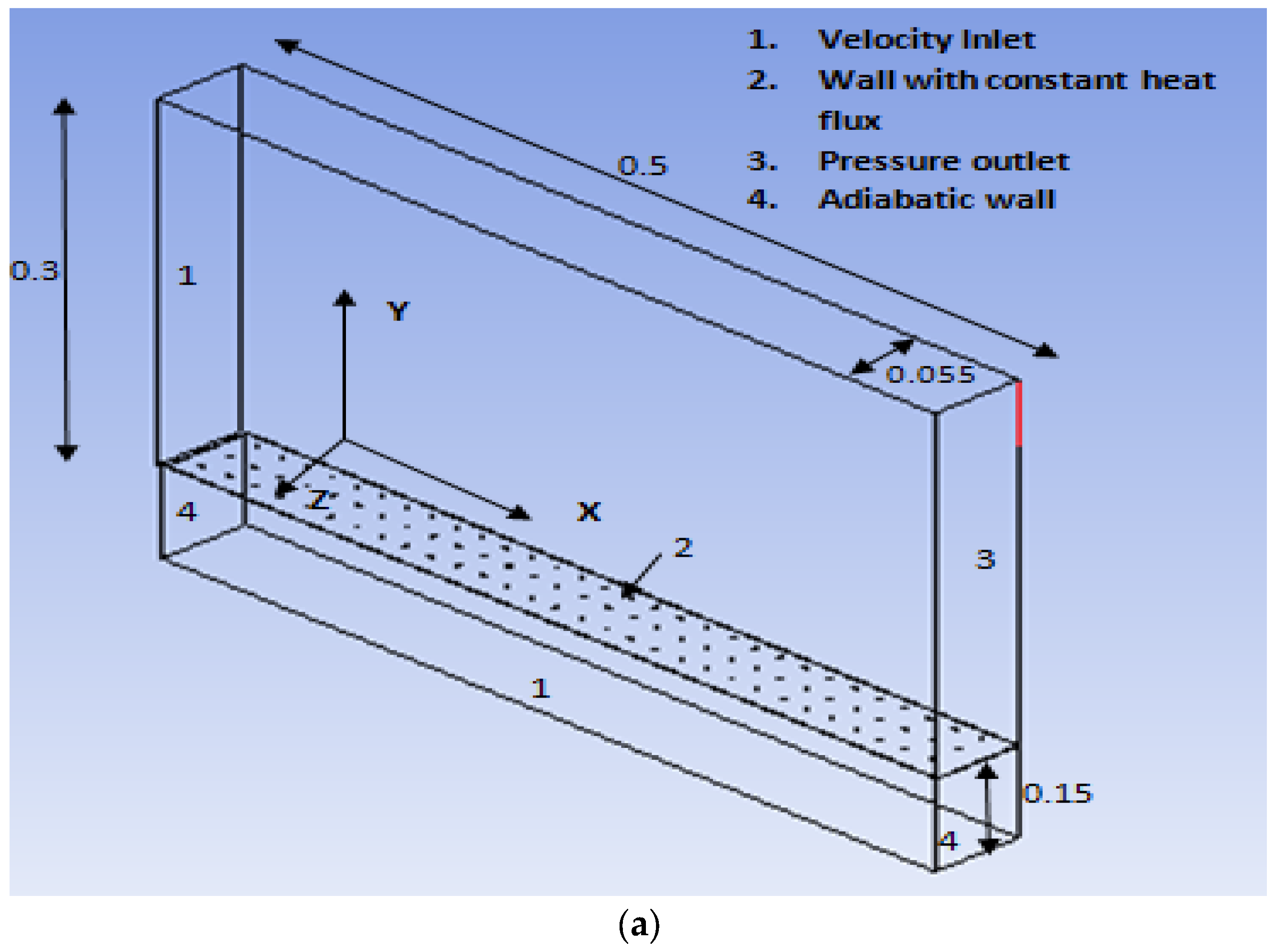
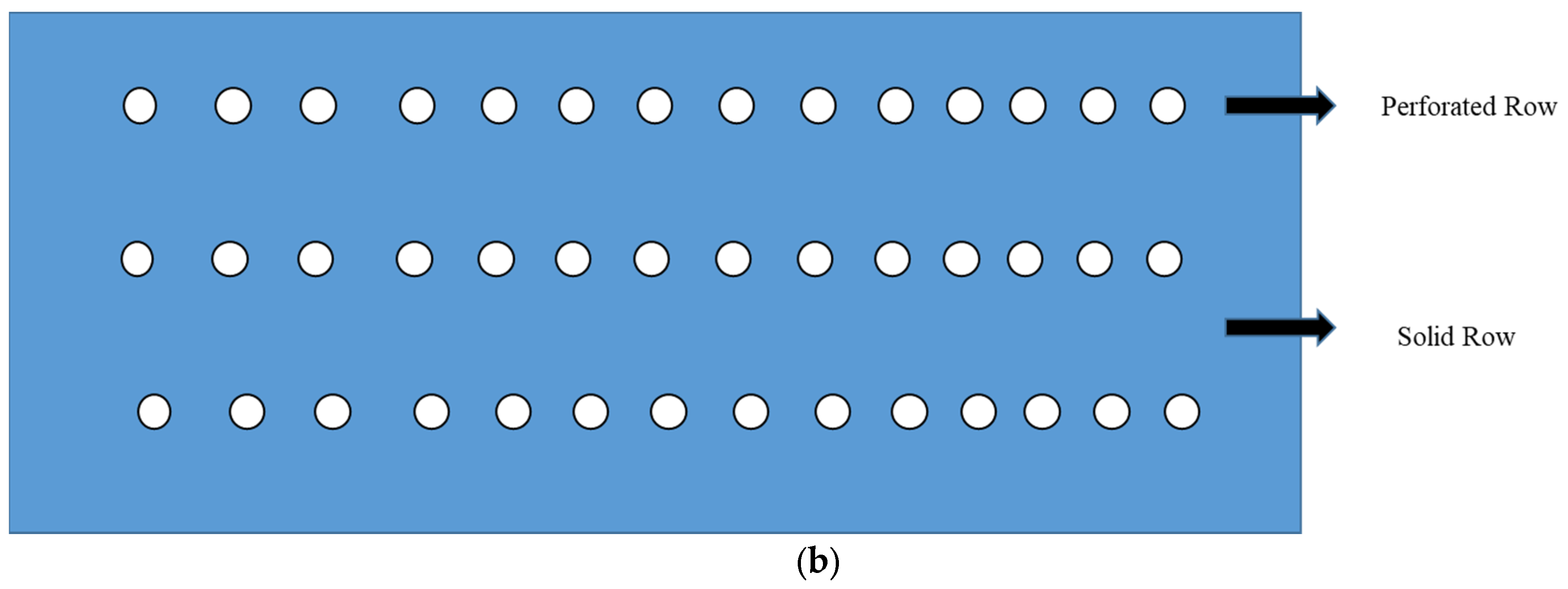
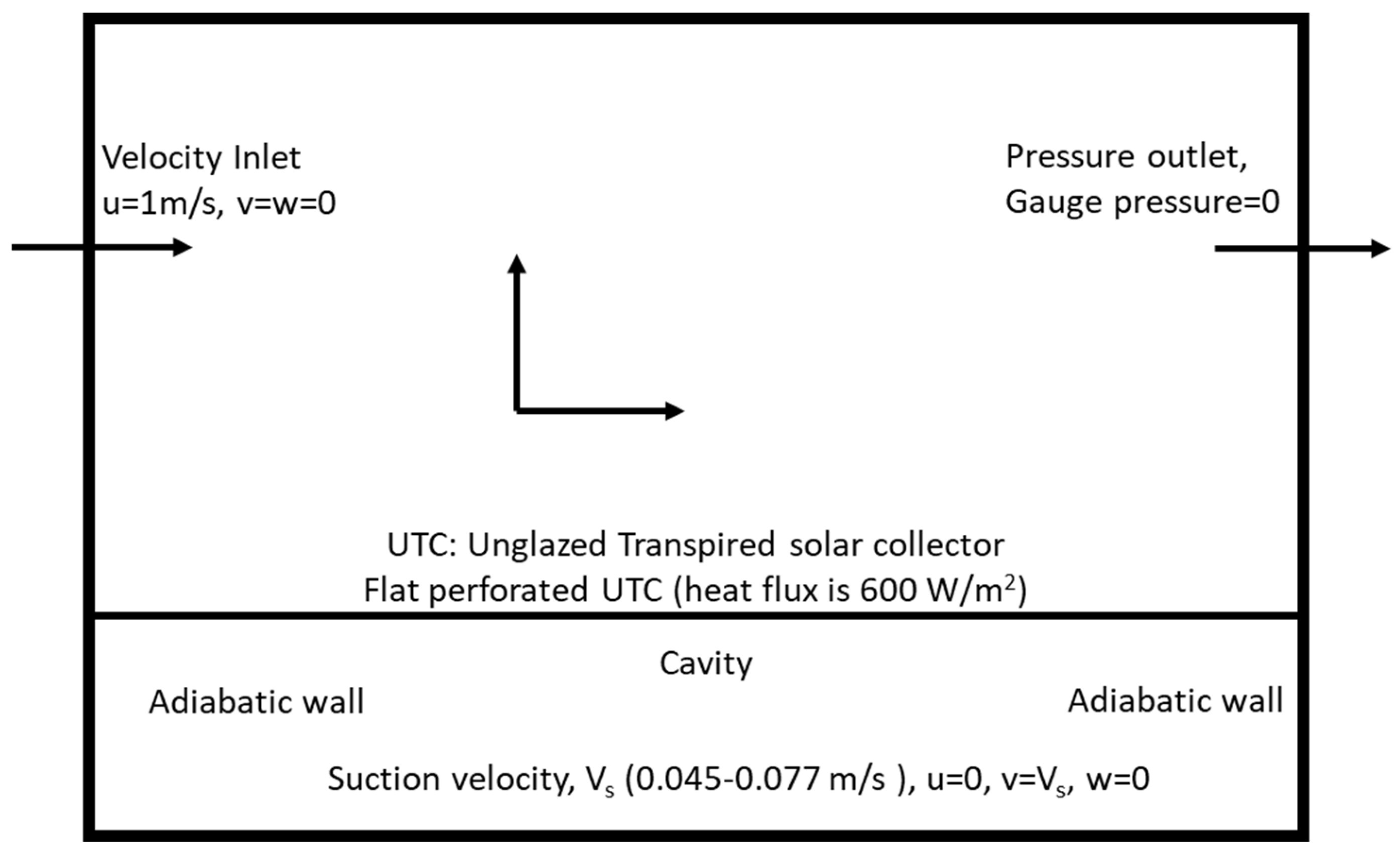
2.1. Modelling
2.2. Mesh Development Analysis
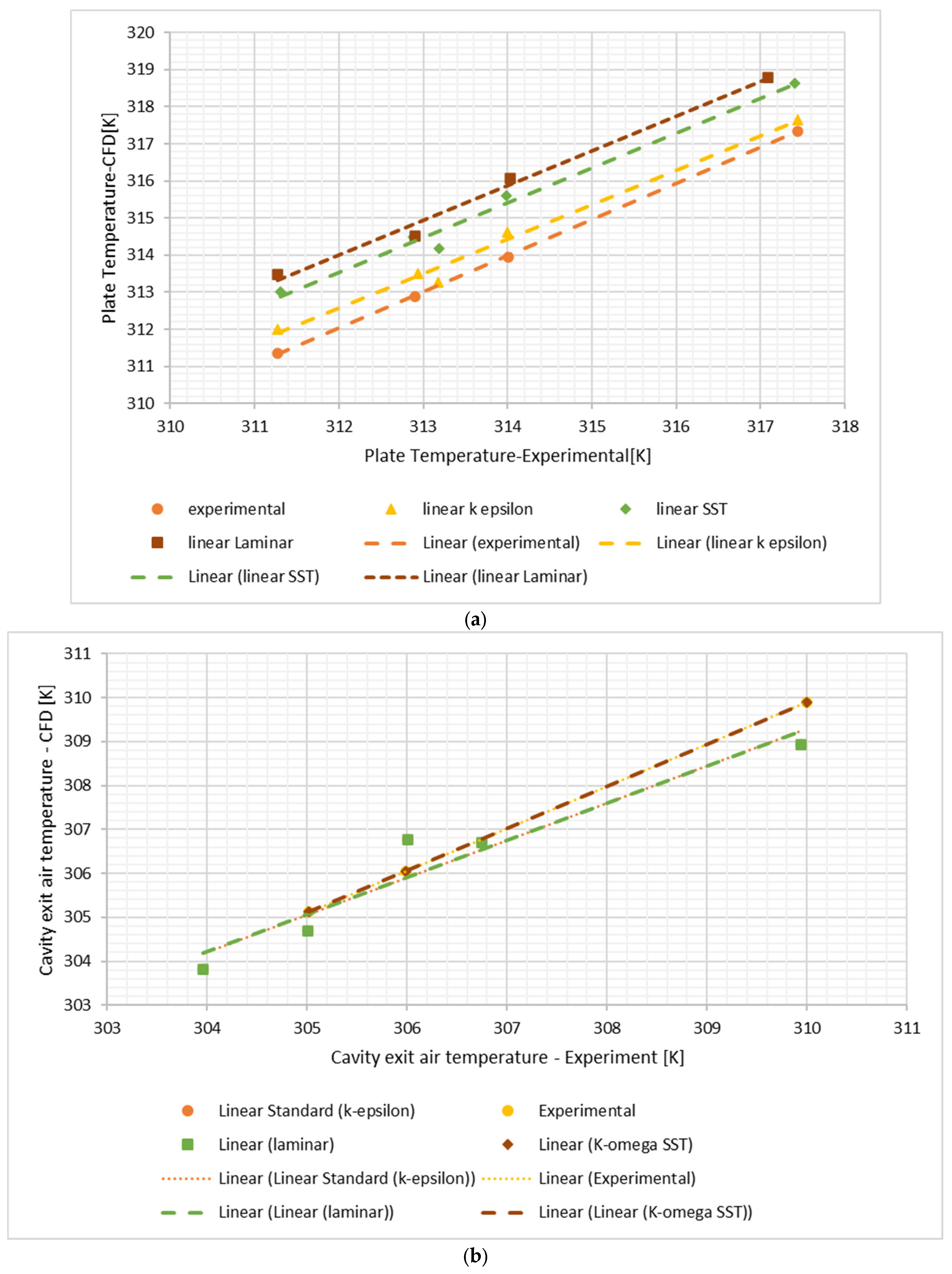
3. Results and Discussion

| Location | Tp | Vy | Te | Tpe | Tee | |
|---|---|---|---|---|---|---|
| Location | 1.00 | 0.29 | −0.84 | −0.12 | 0.33 | −0.16 |
| Tp | 0.29 | 1.00 | −0.07 | 0.04 | 0.99 | 0.06 |
| Vy | −0.84 | −0.07 | 1.00 | 0.35 | −0.11 | 0.37 |
| Te | −0.12 | 0.04 | 0.35 | 1.00 | 0.02 | 1.00 |
| Tpe | 0.33 | 0.99 | −0.11 | 0.02 | 1.00 | 0.05 |
| Tee | −0.16 | 0.06 | 0.37 | 1.00 | 0.05 | 1.00 |
4. Conclusions
Author Contributions
Funding
Acknowledgments
Conflicts of Interest
References
- Li, S.; Karava, P. Evaluation of turbulence models for airflow and heat transfer prediction in BIPV/T systems optimization. Energy Procedia 2012, 30, 1025–1034. [Google Scholar] [CrossRef] [Green Version]
- Li, S.; Karava, P.; Currie, S.; Lin, W.E.; Savory, E. Energy modeling of photovoltaic thermal systems with corrugated unglazed transpired solar collectors—Part 2: Performance analysis. Sol. Energy 2014, 102, 297–307. [Google Scholar] [CrossRef]
- Li, S.; Karava, P.; Savory, E.; Lin, W.E. Airflow and thermal analysis of flat and corrugated unglazed transpired solar collectors. Sol. Energy 2013, 91, 297–315. [Google Scholar] [CrossRef]
- Li, S.; Karava, P.; Currie, S.; Lin, W.E.; Savory, E. Energy modeling of photovoltaic thermal systems with corrugated unglazed transpired solar collectors—Part 1: Model development and validation. Sol. Energy 2014, 102, 282–296. [Google Scholar] [CrossRef]
- Croitoru, C.V.; Nastase, I.; Bode, F.I.; Meslem, A. Thermodynamic investigation on an innovative unglazed transpired solar collector. Sol. Energy 2016, 131, 21–29. [Google Scholar] [CrossRef]
- Vaziri, R.; Ilkan, M.; Egelioglu, F. Experimental performance of perforated glazed solar air heaters and unglazed transpired solar air heater. Sol. Energy 2015, 119, 251–260. [Google Scholar] [CrossRef]
- Collins, M.R.; Abulkhair, H. An evaluation of heat transfer and effectiveness for unglazed transpired solar air heaters. Sol. Energy 2014, 99, 231–245. [Google Scholar] [CrossRef]
- Badache, M.; Rousse, D.R.; Hallé, S.; Quesada, G.; Quesada, G. Experimental and numerical simulation of a two-dimensional unglazed transpired solar air collector. Sol. Energy 2013, 93, 209–219. [Google Scholar] [CrossRef]
- Arulanandam, S.J.; Hollands, K.G.T.; Brundrett, E. A CFD heat transfer analysis of the transpired solar collector under no-wind condition. Sol. Energy 1999, 67, 93–100. [Google Scholar] [CrossRef]
- Panigrahi, S.P.; Maharan, S.K. Correlation of temperature, velocity and perforation location in a flat unglazed transpired solar collector (Utc) due to air flow. JP J. Heat Mass Trans. 2020, 19, 1–18. [Google Scholar] [CrossRef]
- Gawlik, K.M. A Numerical and Experimental Investigation of Heat Transfer Issues in the Practical Utilization of Unglazed, Transpired Solar Air Heaters. Ph.D. Thesis, University of Colorado, Boulder, CO, USA, 1993. [Google Scholar]
- Gawlik, K.M.; Kutscher, C.F. Wind Heat Loss from Corrugated, Transpired Solar Collectors. J. Sol. Energy Eng. 2002, 124, 256–261. [Google Scholar] [CrossRef]
- Iglisch, R. Exact Calculation of Laminar Boundary Layer in Longitudinal Flow over a Flat Plate with Homogeneous Suction; Schriften der Deutschen Akademie der Luftfahrtforschung, Band 8B, Heft 1; NACA: Boston, MA, USA, 1994; Translation: NACA TM No. 1205. [Google Scholar]
- Kutscher, C.; Christensen, C.; Barker, G. Unglazed Transpired Solar Collectors—An Analytical Model and Test-Results. In 1991 Solar World Congress; Arden, M.E., Burley, S.M.A., Coleman, M., Eds.; Elsevier: Amsterdam, The Netherlands, 1992; Volume 2, pp. 1245–1250. [Google Scholar]
- Motahar, S.; Alemrajabi, A.A. An analysis of unglazed transpired solar collectors based on exergetic performance criteria. Int. J. Thermodyn. 2010, 13, 153–160. [Google Scholar]
- Shukla, A.; Nkwetta, D.N.; Cho, Y.J.; Stevenson, V.; Jones, P. A state of art review on the transpired solar collector. Renew. Sustain. Energy Rev. 2012, 16, 3975–3985. [Google Scholar] [CrossRef]
- Kutscher, C.F.; Christensen, C.; Barker, G. Unglazed transpired solar collectors: An analytic model and test results. In Proceedings of the ISES Solar World Congress, Denver, CO, USA, 19–23 August 1991; Elsevier Science: Amsterdam, The Netherlands, 1991; pp. 1245–1250. [Google Scholar]
- Athienitis, A.K.; Bambara, J.; O’Neill, B.; Faille, J. A prototype photovoltaic/thermal system integrated with transpired collector. Sol. Energy 2011, 85, 139–153. [Google Scholar] [CrossRef]
- Dymon, C.; Kutscher, C. Development of a flow distribution and design model for transpired solar collectors. Sol. Energy 1997, 60, 291–300. [Google Scholar] [CrossRef]
- Wang, Y.; Shukla, A.; Liu, S. A state of art review on methodologies for heat transfer and energy flow characteristics of the active building envelopes. Renew. Sustain. Energy Rev. 2017, 78, 1102–1116. [Google Scholar] [CrossRef]
- Skoplaki, E.; Palyvos, J.A. On the temperature dependence of photovoltaic module electrical performance: A review of efficiency/power correlations. Sol. Energy 2009, 83, 614–624. [Google Scholar] [CrossRef]
- Cho, Y.J.; Shukla, A.; Nkwetta, D.N.; Jones, P. Thermal modelling and parametric study of transpired solar collector. In CIBSE ASHRAE Technical Symposium; Imperial College London: London, UK, 2012; pp. 18–19. [Google Scholar]
- Rajashekaraiah, T.; Mura, M.J.; Sharasthantra, R.; Sharma, G.S. Optimizing the efficiency of solar flat plate collector with trapezoidal reflector. AIP Conf. Proc. 2019, 2080, 030008. [Google Scholar]
- Zhang, T.; Tan, Y.; Yang, H.; Zhang, X. The application of air layers in building envelopes: A review. Appl. Energy 2016, 165, 707–734. [Google Scholar] [CrossRef]
- Colangelo, G.; Favale, E.; Miglietta, P.; de Risi, A. Innovation in flat solar thermal collectors: A review of the last ten years experimental results. Renew. Sustain. Energy Rev. 2016, 57, 1141–1159. [Google Scholar] [CrossRef]
- El-Khawajah, M.F.; Aldabbagh, L.B.Y.; Egelioglu, F. The effect of using transverse fins on a double pass flow solar air heater using wire mesh as an absorber. Sol. Energy 2011, 85, 1479–1487. [Google Scholar] [CrossRef]
- Van Decker, G.W.E.; Hollands, K.G.T.; Brunger, A.P. Heat-exchange relations for unglazed transpired solar collectors with circular holes on a square or triangular pitch. Sol. Energy 2001, 71, 33–45. [Google Scholar] [CrossRef]
- Tajdaran, S.; Bonatesta, F.; Ogden, R.; Kendrick, C. CFD modelling of transpired solar collectors and characterisation of multi-scale airflow and heat transfer mechanisms. Sol. Energy 2016, 131, 149–164. [Google Scholar] [CrossRef] [Green Version]
- Li, S.W.; Joe, J.; Hu, J.J.; Karava, P. System identification and model-predictive control of office buildings with integrated photovoltaic-thermal collectors, radiant floor heating and active thermal storage. Sol. Energy 2015, 113, 139–157. [Google Scholar] [CrossRef]
- Semenou, T.; Rousse, D.R.; Le Lostec, B.; Nouanegue, H.F.; Paradis, P.L. Mathematical modelling of dual intake transparent transpired solar collector. Math. Probl. Eng. 2015, 2015, 942854. [Google Scholar] [CrossRef] [Green Version]
- Leon, M.A.; Kumar, S. Mathematical modelling and thermal performance analysis of unglazed transpired solar collectors. Sol. Energy 2007, 81, 62–75. [Google Scholar] [CrossRef]
- Esen, H.; Esen, M.; Ozsolak, O. Modelling and experimental performance analysis of solar-assisted ground source heat pump system. J. Exp. Theor. Artif. Intell. 2017, 29, 1–17. [Google Scholar] [CrossRef]
- Thejaraju, R.; Girisha, K.B.; Manjunath, S.H.; Dayananda, B.S. Numerical evaluation of thermo-hydraulic performance index of a double pipe heat exchanger using double sided louvered winglet tape. J. Therm. Eng. 2020, 6, 843–857. [Google Scholar] [CrossRef]
- Belusko, M.; Saman, W.; Bruno, F. Roof integrated solar heating system with glazed collector. Sol. Energy 2004, 76, 61–69. [Google Scholar] [CrossRef]
- Rounisa, E.D.; Bigaila, E.; Luka, P.; Athienitis, A.; Stathopoulos, T. Multiple-inlet BIPV/T modeling: Wind effects and fan induced suction. Energy Procedia 2015, 78, 1950–1955. [Google Scholar] [CrossRef] [Green Version]
- Belusko, M. Investigation into a Roof Integrated Solar Space Air Heater. Honours Master’s Thesis, University of South Australia, Adelaide, Australia, 1996. [Google Scholar]
- Greig, D.; Siddiqui, K.; Karava, P. An experimental investigation of the flow structure over a corrugated waveform in a transpired air collector. Int. J. Heat Fluid Flow 2012, 38, 133–144. [Google Scholar] [CrossRef]
- Badache, M.; Halle, S.; Rousse, D.R.; Quesada, G.; Dutil, Y. An experimental investigation of a two-dimensional prototype of a transparent transpired collector. Energy Build. 2014, 68, 232–241. [Google Scholar] [CrossRef]
- Ozgen, F.; Esen, M.; Esen, H. Experimental investigation of thermal performance of a double-flow solar air heater having aluminum cans. Renew. Energy 2009, 11, 2391–2398. [Google Scholar] [CrossRef]
- Bejan, A.S.; Teodosiu, C.; Croitoru, C.V.; Catalina, T.; Nastase, I. Experimental investigation of transpired solar collectors with/without phase change materials. Sol. Energy 2021, 214, 478–490. [Google Scholar] [CrossRef]
- Bejan, A.-S.; Croitoru, C.; Bode, F.; Teodosiu, C.; Catalina, T. Experimental investigation of an enhanced transpired air solar collector with embodied phase changing materials. J. Clean. Prod. 2022, 336, 130398. [Google Scholar] [CrossRef]
- Ansys Fluent Theory Guide; Release 2022 R2; Ansys Inc.: Canonsburg, PA, USA, 2022; p. 15317.
- Freedman, D.; Pisani, R.; Purves, R. Statistics (International Student Edition), 4th ed.; Pisani, R., Purves, R., Eds.; WW Norton & Company: New York, NY, USA, 2007. [Google Scholar]
- Saleh, B.; Sundar, L.S.; Aly, A.A.; Ramana, E.V.; Sharma, K.V.; Afzal, A.; Abdelrhman, Y.; Sousa, A.C.M. The Combined Effect of Al2O3 Nanofluid and Coiled Wire Inserts in a Flat-Plate Solar Collector on Heat Transfer, Thermal Efficiency and Environmental CO2 Characteristics. Arab. J. Sci. Eng. 2022, 47, 9187–9214. [Google Scholar] [CrossRef]
- Felemban, B.F.; Essa, F.A.; Afzal, A.; Ahmed, M.H.; Saleh, B.; Panchal, H.; Shanmugan, S.; Elsheikh, A.; Omara, Z.M. Experimental Investigation on Dish Solar Distiller with Modified Absorber and Phase Change Material under Various Operating Conditions. Environ. Sci. Pollut. Res. 2022, 29, 63248–63259. [Google Scholar] [CrossRef]
- Kumar, R.; Nadda, R.; Kumar, S.; Razak, A.; Sharifpur, M.; Aybar, H.S.; Ahamed Saleel, C.; Afzal, A. Influence of Artificial Roughness Parametric Variation on Thermal Performance of Solar Thermal Collector: An Experimental Study, Response Surface Analysis and ANN Modelling. Sustain. Energy Technol. Assess. 2022, 52, 102047. [Google Scholar] [CrossRef]
- Attia, M.E.H.; Thalib, M.M.; Kumar, S.; Afzal, A.; Vaithilingam, S.; Sathyamurthy, R.; Manokar, A.M. Water Quality Analysis of Solar Still Distillate Produced from Various Water Sources of El Oued Region Algeria. Desalin. Water Treat. 2022, 253, 55–62. [Google Scholar] [CrossRef]
- Santhosh Kumar, P.C.; Naveenkumar, R.; Sharifpur, M.; Issakhov, A.; Ravichandran, M.; Mohanavel, V.; Aslfattahi, N.; Afzal, A. Experimental Investigations to Improve the Electrical Efficiency of Photovoltaic Modules Using Different Convection Mode. Sustain. Energy Technol. Assess. 2021, 48, 101582. [Google Scholar] [CrossRef]
- Benoudina, B.; Attia, M.E.H.; Driss, Z.; Afzal, A.; Manokar, A.M.; Sathyamurthy, R. Enhancing the Solar Still Output Using Micro/Nano-Particles of Aluminum Oxide at Different Concentrations: An Experimental Study, Energy, Exergy and Economic Analysis. Sustain. Mater. Technol. 2021, 29, e00291. [Google Scholar] [CrossRef]
- Samylingam, L.; Aslfattahi, N.; Saidur, R.; Mohd, S.; Afzal, A. Solar Energy Materials and Solar Cells Thermal and Energy Performance Improvement of Hybrid PV/T System by Using Olein Palm Oil with MXene as a New Class of Heat Transfer Fluid. Sol. Energy Mater. Sol. Cells 2020, 218, 110754. [Google Scholar] [CrossRef]
- Samuel, O.D.; Kaveh, M.; Oyejide, O.J.; Elumalai, P.V.; Verma, T.N.; Nisar, K.S.; Saleel, C.A.; Afzal, A.; Fayomi, O.S.I.; Owamah, H.I.; et al. Performance Comparison of Empirical Model and Particle Swarm Optimization & Its Boiling Point Prediction Models for Waste Sunflower Oil Biodiesel. Case Stud. Therm. Eng. 2022, 33, 101947. [Google Scholar] [CrossRef]
- Kumar, R.; Nadda, R.; Kumar, S.; Kumar, K.; Afzal, A.; Razak, K.A.; Sharifpur, M. Heat Transfer and Friction Factor Correlations for an Impinging Air Jets Solar Thermal Collector with Arc Ribs on an Absorber Plate. Sustain. Energy Technol. Assess. 2021, 47, 101523. [Google Scholar] [CrossRef]
- Akram, N.; Montazer, E.; Kazi, S.N.; Soudagar, M.E.M.; Ahmed, W.; Zubir, M.N.M.; Afzal, A.; Muhammad, M.R.; Ali, H.M.; Márquez, F.P.G.; et al. Experimental Investigations of the Performance of a Flat-Plate Solar Collector Using Carbon and Metal Oxides Based Nanofluids. Energy 2021, 227, 120452. [Google Scholar] [CrossRef]
- Zare, S.; Ayati, M.; Ha’iriYazdi, M.R.; Kabir, A.A. Convolutional neural networks for wind turbine gearbox health monitoring. Energy Equip. Syst. 2022, 10, 73–82. [Google Scholar]
- Sabzi, S.; Asadi, M.; Moghbelli, H. Review, analysis and simulation of different structures for hybrid electrical energy storages. Energy Equip. Syst. 2017, 5, 115–129. [Google Scholar]


| Surface Number | Boundary Condition Type | Flow Variable |
|---|---|---|
| 1 | Inflow | Flow enters at 1% turbulence with 1 m/s speed at 298 K |
| 2 | Wall | Solar heat flux over wall = 600 W/m2 |
| 3 | Outflow | Open to the atmospheric pressure |
| 4 | Wall | Insulated wall |
| Plate Temperature (K) | Wind Speed and Suction Velocity | Mesh Size | Experimental Data | ||
|---|---|---|---|---|---|
| Mesh 1 | Mesh 2 | Mesh 3 | |||
| Case Study 1 | 1 m/s & 0.077 m/s | 314/305.9 | 314.5/305.7 | 314.7/305.0 | 313.9/306.5 |
| Case Study 2 | 1 m/s & 0.045 m/s | 315.4/307 | 314.8/307.1 | 313.7/306.9 | 313.9/306.5 |
Publisher’s Note: MDPI stays neutral with regard to jurisdictional claims in published maps and institutional affiliations. |
© 2022 by the authors. Licensee MDPI, Basel, Switzerland. This article is an open access article distributed under the terms and conditions of the Creative Commons Attribution (CC BY) license (https://creativecommons.org/licenses/by/4.0/).
Share and Cite
Parimita Panigrahi, S.; Kumar Maharana, S.; Rajashekaraiah, T.; Gopalashetty, R.; Sharifpur, M.; Ahmadi, M.H.; Saleel, C.A.; Abbas, M. Flat Unglazed Transpired Solar Collector: Performance Probability Prediction Approach Using Monte Carlo Simulation Technique. Energies 2022, 15, 8843. https://doi.org/10.3390/en15238843
Parimita Panigrahi S, Kumar Maharana S, Rajashekaraiah T, Gopalashetty R, Sharifpur M, Ahmadi MH, Saleel CA, Abbas M. Flat Unglazed Transpired Solar Collector: Performance Probability Prediction Approach Using Monte Carlo Simulation Technique. Energies. 2022; 15(23):8843. https://doi.org/10.3390/en15238843
Chicago/Turabian StyleParimita Panigrahi, Sajna, Sarat Kumar Maharana, Thejaraju Rajashekaraiah, Ravichandran Gopalashetty, Mohsen Sharifpur, Mohammad Hossein Ahmadi, C. Ahamed Saleel, and Mohamed Abbas. 2022. "Flat Unglazed Transpired Solar Collector: Performance Probability Prediction Approach Using Monte Carlo Simulation Technique" Energies 15, no. 23: 8843. https://doi.org/10.3390/en15238843