1. Introduction
The gas turbine plays an important role in CCPP (combined cycle power plants) and is largely composed of a compressor, a combustor, and turbine. Compressors rotating at a high speed cause surge or vibration problems and combustors have problems such as thermodynamic stress or combustion vibration due to high temperature and high flow rate. Turbines have problems such as coating detachment due to the high temperatures and pressures coming from the combustor. Therefore, gas turbines are very sensitive pieces of industrial equipment, and only a preemptive response to various issues can ensure gas turbine operability, maintainability, and performance.
A concept introduced for the overall health management of gas turbines is PHM (prognosis and health management). Because PHM is directly related to the three issues mentioned above (operability, maintainability, and continuous performance), it is a very important technology, not only for gas turbine OEMs, but also for customers. OEMs can gain product trust from customers through PHM, and, on the contrary, customers can expect stable power via PHM.
Recently, PHM and AI technology have been combined and developed in various ways. The purpose of using PHM and AI technology together is to analyze real-time gas turbine data, detect unexpected prognoses, and act to avoid them by means of a preventive maintenance schedule. The first act of PHM via AI technology is failure diagnosis, which predicts anomalies based on the numerous data generated from gas turbines. A OC-SVM (one-class support vector machine) is a commonly used algorithm for determining system abnormalities.
Takahiro et al. [
1] analyzed failure detection accuracy using OC-SVM to detect defects in the gas turbine generator of the thermal power plant. In particular, OC-SVM method demonstrated an accuracy of up to 98% for defect detection. Weizhong et al. [
2] conducted a study applying one of the latest technologies, using an extreme learning machine (ELM) technique, to a OC-SVM in order to detect abnormalities in gas turbines combustors. By way of the advantages of OC-SVM, combined with maintaining the advantages of ELM, better performance results can be obtained than those with the use of other classification models. Ioannis et al. [
3] conducted a fault diagnosis study using gas turbine vibration data. Among the hyperparameters of the OC-SVM, the width
and optimization penalty parameters (
) of the kernel were optimized using a grid search method. As a result of the optimization, the accuracy of the model was close to 100%, and the optimization of the hyperparameter was emphasized to improve the model accuracy. Daogang et al. [
4] conducted a study on the failure diagnosis of various sensor data inputs to the gas turbine control system using a SVM. The characteristics of the data were extracted using an EMD (empirical mode decomposition) method, and a fault diagnosis model was constructed using a SVM. As a result, the algorithm accuracy for randomly selected variables reached up to 85%. Weihong et al. [
5] analyzed the vibration signal of a gas turbine bearing and conducted a study to separate the operating state and failure type using a OC-SVM. An algorithm to effectively diagnose the bearing state and soundness, even in a small sample environment, was proposed by extracting the characteristic signal of the bearing and applying it to a SVM algorithm.
Unsupervised OC-SVMs are used in a variety of fields besides gas turbine systems (see
Figure 1). Takashi et al. [
6] conducted a study to detect abnormal signs of hydroelectric power plants using OC-SVM. A method of predicting the failure of a hydroelectric power plant was proposed by determining the abnormal vibration phenomenon of the bearing among various sensor data. Juhamatti et al. [
7] used a OC-SVM algorithm to diagnose wind turbine failures. OC-SVM performance changes according to changes in the values of
and
were analyzed to diagnose bearing failures from the vibration signals extracted from the wind turbines. So far, several studies have been conducted to improve the anomaly detection performance of OC-SVM. Even with the same algorithm, the prediction accuracy can be increased by adding a special algorithm in the variable selection stage. In addition, by optimizing the various hyperparameters of the OC-SVM, the algorithm accuracy may be improved by up to 10% or more.
In this study, anomaly detection study is performed using gas turbine data. A OC-SVM algorithm is used, where the main purpose is to increase the prediction accuracy by tuning the hyperparameter of the OC-SVM. Four methods are used for hyperparameters tuning, including manual searching, grid searching, random searching, and Bayesian optimization. Through the combined above method, the accuracy of the OC-SVM is improved by more than 10% when compared to the initial algorithm.
2. Methodology of One-Class Support Vector Machine (OC-SVM)
A support vector machine (SVM) is a method for generating criteria for classifying data sets [
8,
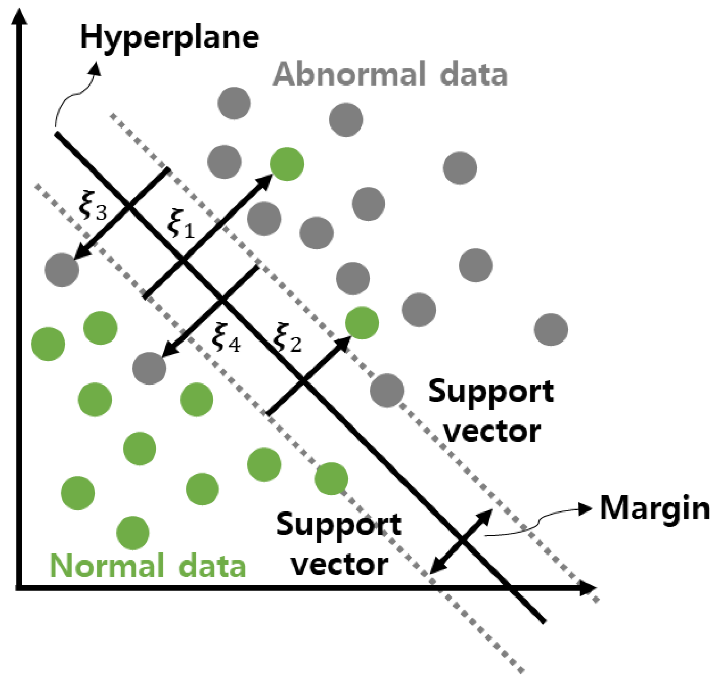
9]. In this case, the criterion used is referred to as a decision boundary or a hyperplane. Based on this, data types with different features are classified. The data closest to the hyperplane is called a support vector. As shown in
Figure 2, the two points closest to the hyperplane are designated as support vectors, respectively. The margin is the distance between the support vector and the hyperplane. Therefore, the goal of improving the support vector machine performance is to find the hyperplane that maximizes the margin.
Classification problems can be divided into one-class classification and multi-class classification. The standard for this is the data class used in the training process. For example, if a classification process is performed after training only one class, it is included in the one-class classification process.
In this study, after training using only normal data, data sets not included in the relevant criteria correspond to one-class classification, which is classified as abnormal. Therefore, the main purpose of a OC-SVM is to classify normal data and outlier data by constructing a hyperplane with the maximum margin using the kernel function
to high-dimensionalize the input data. The objective function of the OC-SVM is as Equation (1) [
10], where
is a term that is regularized to minimize the fluctuation caused by the change in
, and
is the distance between the origin and the hyperplane. Minimization of the objective function can be reached by maximizing
. Further,
is the sum of the penalty
given to normal data,
denotes the number of normal data, and
means the smoothness of the boundary, and
is a slack variable and has the same relational expression as Equation (2). If a hyperplane to discriminate data is found using the objective function, a decision boundary such as Equation (3) is used to classify normal data as positive number and abnormal data as negative number based on this. In this study, the gas turbine dataset is classified into normal/abnormal using OC-SVM. In addition, four hyperparameter tuning processes, which will be mentioned in the next section, are used to improve the fault diagnosis performance.
3. Hyperparameter
In this paper, four hyperparameter tuning techniques (manual search, grid search, random search, and Bayesian optimization) are applied to improve the performance [
11,
12]. The kernel function uses a Gaussian kernel (radial basis function), and the hyperparameters were set to
and
. A kernel function is a function that increases efficiency through high-dimensional mapping effect for non-linear datasets that are difficult to classify. Among them, this study uses the most generalized Gaussian kernel. The form for the Gaussian kernel function is given as Equation (4), and
means variance [
13].
Note that
is a variable that determines how much tolerance is given in the classification process, and the allowable range is set based on the support vector. A large
-value means that the tolerance is small. In this case, overfitting occurs. On the other hand, a small number means a wide acceptable range, and it is difficult to accurately classify complex data, resulting in poor reliability.
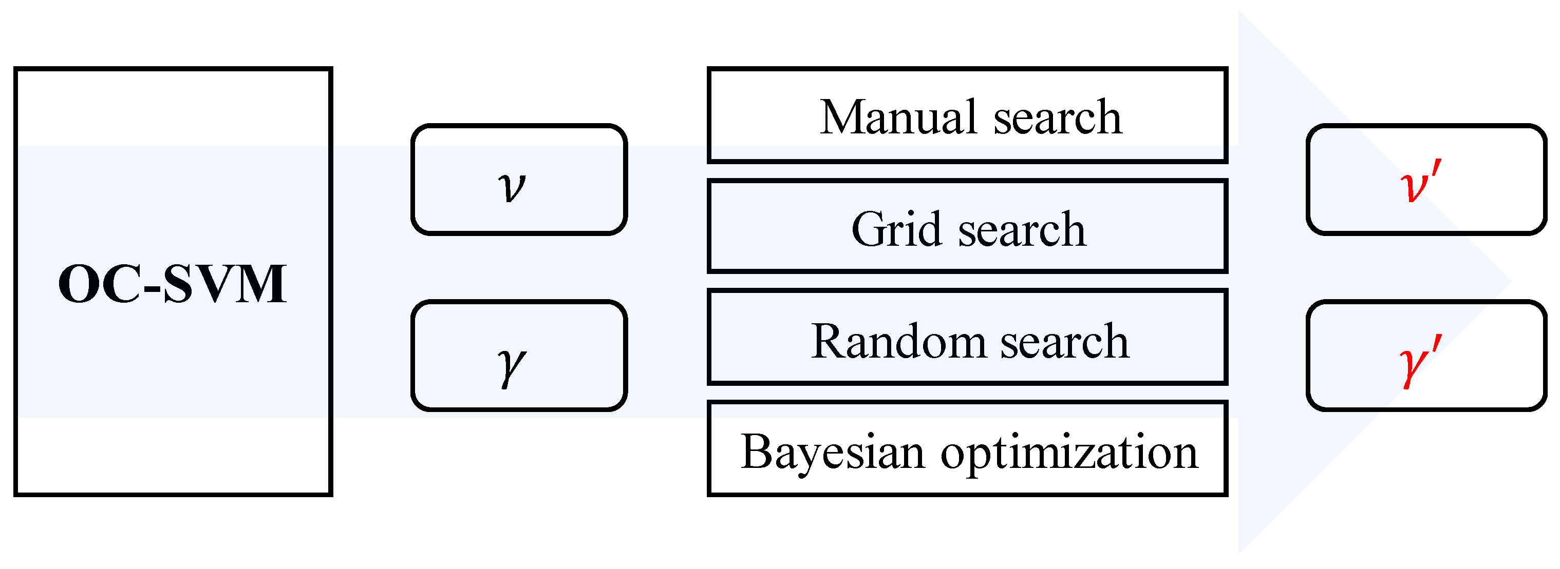
controls the smoothness of the kernel function. The larger
, the smoother the function. As the classification performance varies according to the two hyperparameters (
,
), optimization was performed with the following advanced method. The overall hyperparameter tuning process is shown in
Figure 3. Therefore, the purpose of this study is to derive
′ and
′ in improved performance through four tuning techniques.
3.1. Manual Search
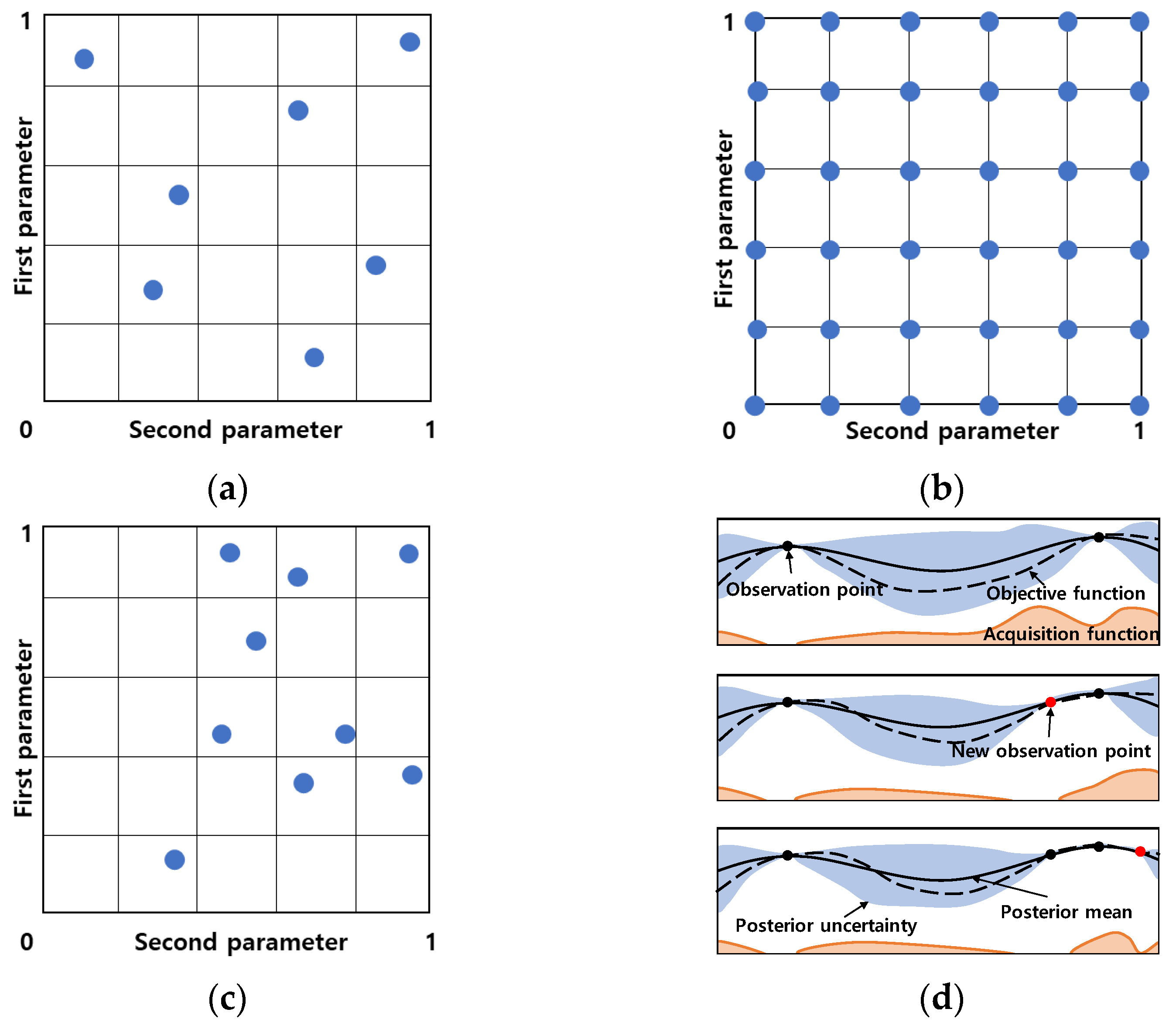
This method is a method of deriving the optimal performance by inputting numerical values arbitrarily (see
Figure 4a). After training by substituting a numerical value, the user sees the obtained result and re-enters the value according to the user’s judgment. It is an empirical tuning method without set rules, so it has the advantage of taking less time. However, in order to derive high performance, there is a large difference depending on individual ability, and there are limitations in that it is difficult to search for major hyperparameters in various ways. Therefore, this method is mainly used when there are few parameters and stops when a target value is obtained within a given time. In this paper, after setting arbitrary values for two hyperparameters (
,
), the training proceeds by repeatedly substituting the values.
3.2. Grid Search
This method derives a combination of rules for hyperparameters using the Cartesian product (see
Figure 4b). In the iterative process, the result corresponding to each situation is derived without reflecting the previous result. After setting the range for the hyperparameter to be applied in advance, it is a method to find the optimal combination considering the number of all cases. The wider the range and the smaller the interval, the greater the probability of finding the optimal solution. On the other hand, as the range is narrowed and the interval is set, the probability of finding the optimal combination decreases, but the time required is short. Mainly, the latter method is used to gradually decrease the range. Therefore, it is effective when the number of hyperparameters is small. In this paper, a combination was created through the Cartesian product for two hyperparameters (
,
). Variables corresponding to
were designated using i, and variables corresponding to
were designated using j. Variable i is set to consist of 100 elements, and variable j is set to consist of 1000 elements. Through this combination, a total of 100 × 1000 combinations were learned, and the optimal combination was found.
3.3. Random Search
In the case of grid search, a relatively accurate optimal solution can be derived because all combinations of the range set using the Cartesian product are trained, but it has the disadvantage that it takes a lot of time. To compensate for this, a random search method was applied. Random search is a method for training by deriving hyperparameter values randomly within a range after the user specifies the minimum and maximum values of the hyperparameter (see
Figure 4c). Compared to grid search, the training speed is faster, and it has the advantage of being able to learn points other than the points specified by the user. In this study, random search was performed using the “randomized search CV” function. For each of the hyperparameters
and
, the minimum and maximum sections were set as shown in Equation (5) below. The number of iterations was set to 100,000, and training was performed with a total of 500,000 samples through 5-fold cross-validation.
3.4. Bayesian Optimization
The three advanced techniques mentioned above are independent methods that do not reflect the results for each point. There is a lack of credibility in the results obtained through training. To supplement this, the Bayesian optimization method, an optimization method made by combining Bayesian theory and a Gaussian process was used (see
Figure 4d).
In the case of Bayesian theory, the relationship between the prior probability and posterior probability of two variables is explained. Referring to Equation (6), the posterior probability
can be obtained when the values of the prior probability p(A) and the likelihood
are known.
A Gaussian process is a distribution over a function. As the multi-variate normal distribution is expressed by the mean vector and the covariance matrix, the Gaussian process is defined as the following Equation (7) through the mean function and the covariance function. The Gaussian process is used as a prior in Bayesian theory.
Bayesian optimization is a hyperparameter tuning process that derives the maximum or minimum value of a function by introducing the concept of a black-box function rather than a clearly presented function to the objective function. The process proceeds in two stages (surrogate function and acquisition function). First, after training the surrogate function for estimating the objective function, the direction of selecting the improved hyperparameter condition is presented. Among the various surrogate models, the most representative method is the Gaussian process regression described above. The function that calculates the hyperparameter condition to be substituted from the result of the surrogate model is the acquisition function. Acquisition functions are also classified into two types (exploration and exploitation). Exploration is a method of exploring uncertain points by focusing on conditions with large variance. That is, when the objective function is verified using a new point, the prior distribution of the new objective function is updated. Exploitation focuses on the high mean (the best point within a known range). That is, based on the posterior distribution, training is performed at the location with the highest probability of being the global minimum point. In other words, the Gaussian process for the black-box function is applied using the extracted training data using Bayesian optimization, and the next data is extracted in a direction that can minimize the uncertainty of the objective function. After that, the minimum or maximum value of the objective function is calculated by repeating the process. In this study, a Bayesian optimization process was performed by setting a total of 1,000,000 iterations for the same two hyperparameters (, ) as in the previous three methods.
5. Conclusions
In this study, the anomaly detection performance of gas turbines, which plays an important role in CCPP, was improved. Actual gas turbine data composed of seven tags provided by Doosan Enerbility in Korea were used. The data consist of a total of about 8000 data points, most of which are normal data and contain a small amount of abnormal data. Since training was performed for one class, anomaly detection was performed using OC-SVM, which has an advantage in classification in the corresponding data set. Additionally, four types of hyperparameter tuning (manual search, grid search, random search, and Bayesian optimization) were applied to improve the performance. The hyperparameter was set to and . Performance evaluation was performed for analysis between tuning techniques. Four indicators were set as accuracy, precision, recall, and F-1 score. In the case of manual search, an accuracy of 0.5429 and F-1 score of 0.6242 were recorded ( = 0.001, = 0.9). In the case of grid search, an accuracy of 0.6038 and F-1 score of 0.6262 were obtained (= 0.6, = 0.09). In the case of random search, an accuracy of 0.6381 and F-1 score of 0.6301 were recorded ( = 0.2185 and = 0.5945). Bayesian optimization performed best, with an accuracy of 0.6488 and F-1 score of 0.6371. That is, = 0.4309 and F-1 score = 0.55521 corresponding to Bayesian optimization were the optimal hyperparameter combinations. Finally, the Bayesian optimization method made by combining Bayesian theory and Gaussian process had the highest anomaly detection performance for the corresponding dataset.

 ,
, 


