Article

Artificial Intelligence Model in Predicting Geomechanical Properties for Shale Formation: A Field Case in Permian Basin

1
Petroleum Engineering Program, Texas A&M International University, Laredo, TX 78041, USA
2
School of Computing and Informatics, University of Louisiana at Lafayette, Lafayette, LA 70503, USA
3
Systems Engineering Program, Texas A&M International University, Laredo, TX 78041, USA
*
Author to whom correspondence should be addressed.
Energies 2022, 15(22), 8752; https://doi.org/10.3390/en15228752
Submission received: 31 October 2022 / Revised: 14 November 2022 / Accepted: 18 November 2022 / Published: 21 November 2022
(This article belongs to the Special Issue Application of Machine Learning in Rock Characterization)

Abstract

:
Due to complexities in geologic structure, heterogeneity, and insufficient borehole information, shale formation faces challenges in accurately estimating the elastic properties of rock which triggers severe technical challenges in safe drilling and completion. These geomechanical properties could be computed from acoustic logs, however, accurate estimation is critical due to log deficit and a higher recovery expense of inadequate datasets. To fill the gap, this study focuses on predicting the sonic properties of rock using deep neural network (Bi-directional long short-time memory, Bi-LSTM) and random forest (RF) algorithms to estimate and evaluate the geomechanical properties of the potential unconventional formation, Permian Basin, situated in West Texas. A total of three wells were examined using both single-well and cross-well prediction algorithms. Log-derived single-well prediction models include a 75:25 ratio for training and testing the data whereas the cross-well includes two wells for training and the remaining well was used for testing. The selected well input logs include compressional wave slowness, resistivity, gamma-ray, porosity, and bulk density to predict shear wave slowness. The results using RF and Bi-LSTM show a promising prediction of geomechanical properties for Permian Basin wells. RF algorithm performed superior for both single and grouped well prediction. The single-well prediction method using the RF algorithm provided the highest accuracy of 99.90% whereas Bi-LSTM gave 93.60%. The best accuracy for a grouped well prediction was achieved employing Bi-LSTM and RF models, i.e., 96.01% and 93.80%. The average prediction including RF and Bi-LSTM algorithms demonstrated that accuracy for single well and cross well prediction is 96% and 94% respectively with an error below 7%. These outcomes show the astonishing capability of artificial intelligence (AI) models trained to create a realistic prediction to unlock unconventional potential when datasets are inadequate. Given adequate training data, operators could leverage these efficient tools by utilizing them to examine fracture interpretations with reduced cost and time when datasets are incomplete and thus increase the hydrocarbon recovery potential.

1. Introduction

The safety and success of hydrocarbon resource exploration depend on the accurate estimation of the geomechanical properties. Geomechanical properties thus play an essential role in developing conventional and unconventional reservoirs [1]. However, accurate estimation is challenging due to complexities in geologic structure, heterogeneity, and insufficient borehole information [2]. Existing analytical methods are time-consuming and very expensive, requiring extensive transformations and lengthy laboratory tests. In addition, reliable target zone identification during the exploration requires accurate location identification [3].
Geomechanical properties locate the sweet spots for fracturing, which is crucial for hydrocarbon recovery from complex formations [4]. They are obtained from the compressional and shear wave slowness data, which augments the accuracy of hydrocarbon production and fluid detection prediction. Geomechanical properties calculation requires acoustic logs, including compressional travel time (DTC) and shear travel time (DTS). The sonic data are usually acquired through an acoustic log or from core samples using laboratory testing.
However, the complication of the process, along with the lack of information on the borehole, makes it very challenging and time-consuming to obtain reliable logging data, resulting in higher recovery costs and incomplete data sets with a log deficiency [5,6]. Different empirical and petrophysical models are used for predicting shear wave velocity for different types of reservoirs, including mudstone structures [7,8,9,10], requiring robust data sets that include mineral composition, pore structure, and fluid parameters. However, due to several factors and limitations, empirical correlations cannot be easily selected. Poor prediction of sonic logs using the empirical correlations and elastic parameters of rocks estimation will be erroneous, leading to big financial issues [11]. Therefore, it is important to reconstruct missing and/or distorted log sections during formation evaluation and reservoir characterization.
During logging operations, broken or faulty tools can lead to many errors. It could take measurements of a few zones, thereby avoiding other potential pay zones; thus, contributing entirely erroneous data suite. So, it is necessary to rebuild missing and/or inaccurate log sections during reservoir characterization and prospect evaluation. According to Castagna, using formation-specific and regression-based correlations, shear wave velocity (Vs) can be estimated from the compressional velocity (Vp) [8]. On the other hand, Brocher predicted vs. from the Vp, but there is a limitation for the Vp range [12], which trigger more investigation on acoustic logging.
In recent years, the use of artificial intelligence (AI) has been increasing extensively for a wide range of engineering and industrial purposes [13,14]. Among them, one of the fastest-growing sectors is the petroleum industry. This tool is predominantly used for the estimation and optimization of petrophysical properties [15,16,17,18,19], geomechanical properties [20,21,22], reservoir fluid properties [23,24,25,26,27,28], and parameters related to drilling [29,30,31,32,33,34,35,36,37]. Researchers employed different ML methods, including an artificial neural network, fuzzy logic, functional network, etc. to predict and analyze geomechanical properties [38,39,40,41,42,43,44,45,46]. The studies reveal that different types of formation differ significantly in behavior, and rock mechanical properties are more complex than ideal materials.
There is a knowledge gap in terms of the unavailability of algorithms for predicting DTS, especially for the formation with distinct geologic heterogeneity, even with the advances in the data-driven artificial neural networks applied in the petroleum field. However, for the effective prediction of sequential data, the use of the Bi-LSTM model has been reported [47].
The Permian Basin located in the West Texas region become one of the most productive energy regions in the world. The geographic region is shown in Figure 1. The basin reserve is reported about 92.3 billion barrels of oil and 300 trillion cubic feet of natural gas which is 38 times Alaska’s reserves and forecasted capable of meeting U.S. energy demand for 60 years [48]. However, the basin continuously faces severe technical challenges during the drilling, completion, and fracturing. In addition, there is a knowledge gap in terms of the lack of an accurate method for estimating the elastic characteristics of the formation, which is vital for safely and efficiently executing the drilling and completion program [49].
This study focuses on a handy and easy-to-use artificial neural network (ANN) model that is capable of predicting missing or incomplete information. To accomplish this objective, two ANN models were applied to forecast shear travel slowness (DTS) from different input log data. Supervised deep neural network, Bi-LSTM, and classical ML model random forest (RF) algorithm were employed to predict the shear wave slowness.
Prediction of the acoustic data accurately will give dependable data on the reservoirs’ elastic properties. This study elaborates an ancillary method for forecasting reservoir elastic properties using the predicted acoustic data when data sets are incomplete or absent. The model results of the two models were then compared to examine the model’s efficacy.
Therefore, accurate prediction of the ANN-based models developed in this study will address the knowledge gap. There is a significant improvement in both the treatment design and the role of the geomechanicist with the adoption of the ML algorithms developed in this study. Further, the operator can utilize the ML or AI models to audit the fracture interpretations, saving costs and reducing time.

2. Methodology

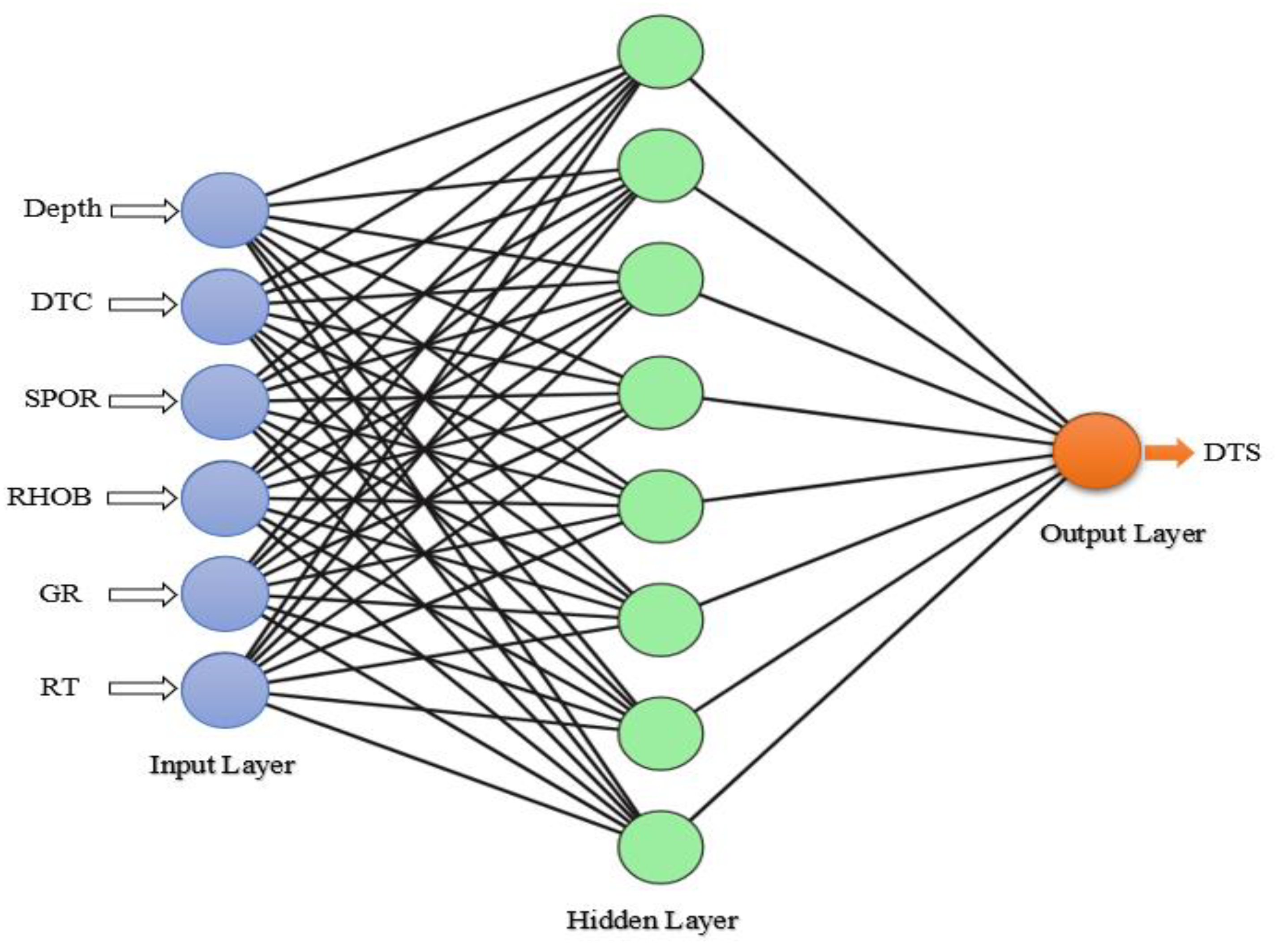
ANN is an effective tool for constructing relationships between non-linear constraints in the absence of abundant data in its structure. The log-derived prediction algorithm includes porosity, bulk density, compressional travel time, gamma-ray, and resistivity as input to predict shear travel time. Then, ML and deep learning algorithms were used to predict DTS. Finally, dynamic Young’s modulus, Poisson’s ratio, and minimum horizontal stress are estimated using the petrophysical correlation with predicted DTS value and compared. A total of two prediction methods are used to predict DTS value: single well and cross well prediction.
(a)
In a single-well prediction, from the log data, 75% is used for training, and the remaining 25% for testing, as illustrated from the workflow in Figure 2.
(b)
Similarly, for a grouped or cross-well prediction (a group of wells from an identical region), the data from two wells were used for training and the remaining third well for testing. The three Permian Basin wells’ log data used for this study are illustrated by the workflow in Figure 3. In this case, the test data are completely unknown to trained models since the model is trained by another two wells from two different regions.
Figure 2. Workflow for estimating geomechanical properties.
Energies 15 08752 g002
Figure 3. Algorithm for cross-well prediction.
Energies 15 08752 g003
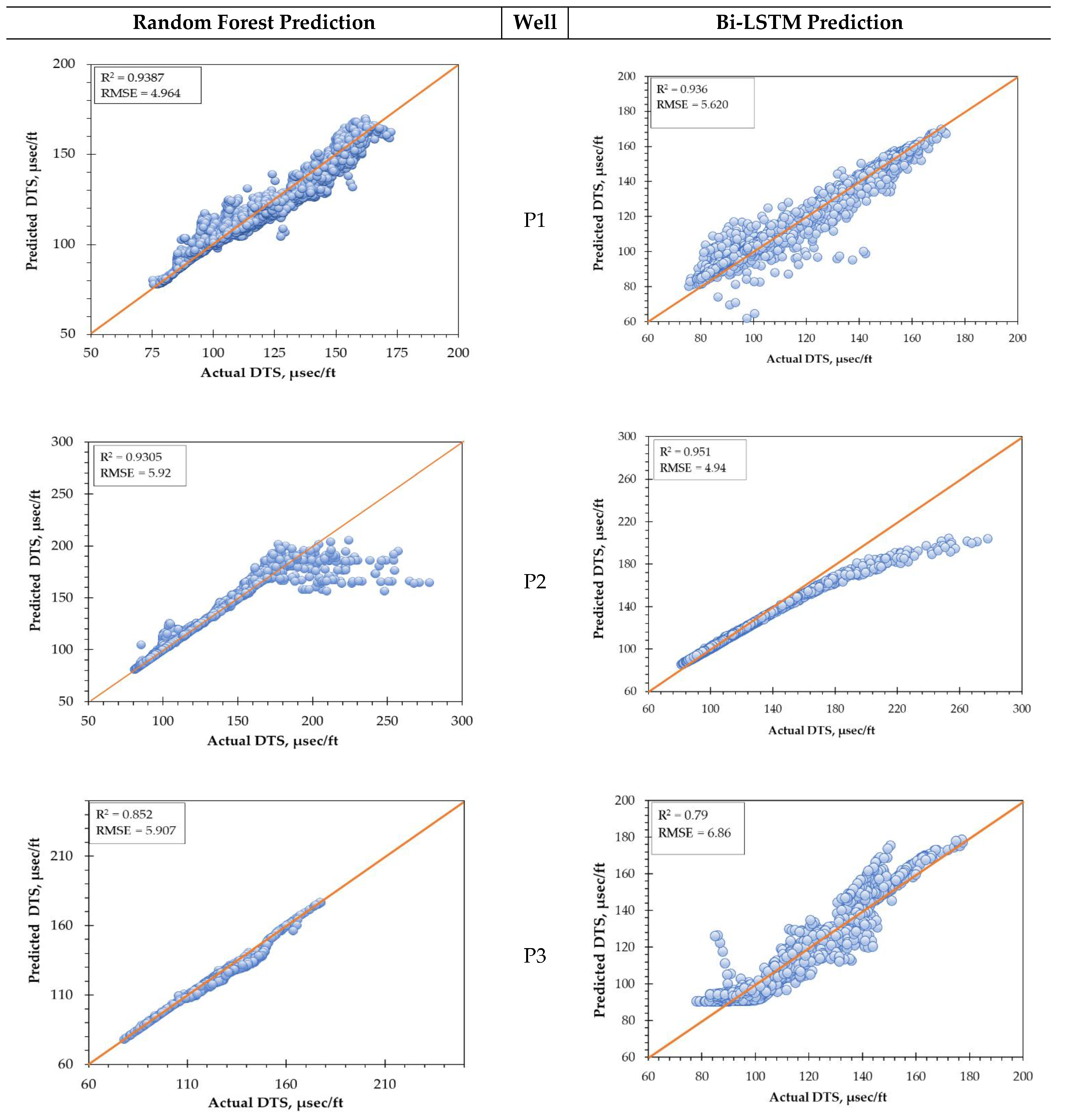
We used both the ML algorithm random forest (RF) and a Bi-LSTM to examine and compare the effectiveness of the prediction of geomechanical properties. Finally, we calculated the average of both ML models’ results to generate a safe and realistic prediction.

2.1. Machine Learning Algorithm

Random Forest: RF is an algorithm based on the decision tree which is used particularly for providing precise and easy-to-interpret outcomes which are fit for purpose.
RF operates by constructing several decision trees from various subsets of data. The model prediction is achieved by voting on the outcomes of multiple decision trees. (RF) is implemented using the standard Python library [51]. We used the “RandomizedSearchCV” library from Sklearn to optimize our hyperparameters for RF and found the optimized parameter, where the estimator = 50, max features = ‘sqrt’ cross well, and max depth = 260. We also changed these hyper-parameters for single wells and reported the results.

2.2. Deep Learning Mechanism

Bidirectional long short-term memory (Bi-LSTM): The current study's dataset is depth-wise sequential. The prediction of the new dataset requires long-term dependencies. The architecture of the LSTM model can learn patterns with long dependencies where the conventional RNN models are not capable to perform for long-term relationships and patterns [52,53,54]. During time series data prediction, LSTM has usually been found to outperform RNNs. Thus, here, the LSTM model is employed as it is capable of capturing both the temporal and spatial characteristics of the selected wells.
We defined a bi-directional LSTM layer with 50 neurons and set the batch size to 5. To reduce the overfitting of the data, a dropout layer of 25% is applied after the first layer of the Bi-LSTM model. ReLU is employed as the activation function. For the number one layer, the Adam optimizer and MSE loss function are used in the current model and one predicted output was in the last dense layer. During the training of the data, the model iterated over 20 epochs. The ANN model employed in this study is presented in Figure 4.
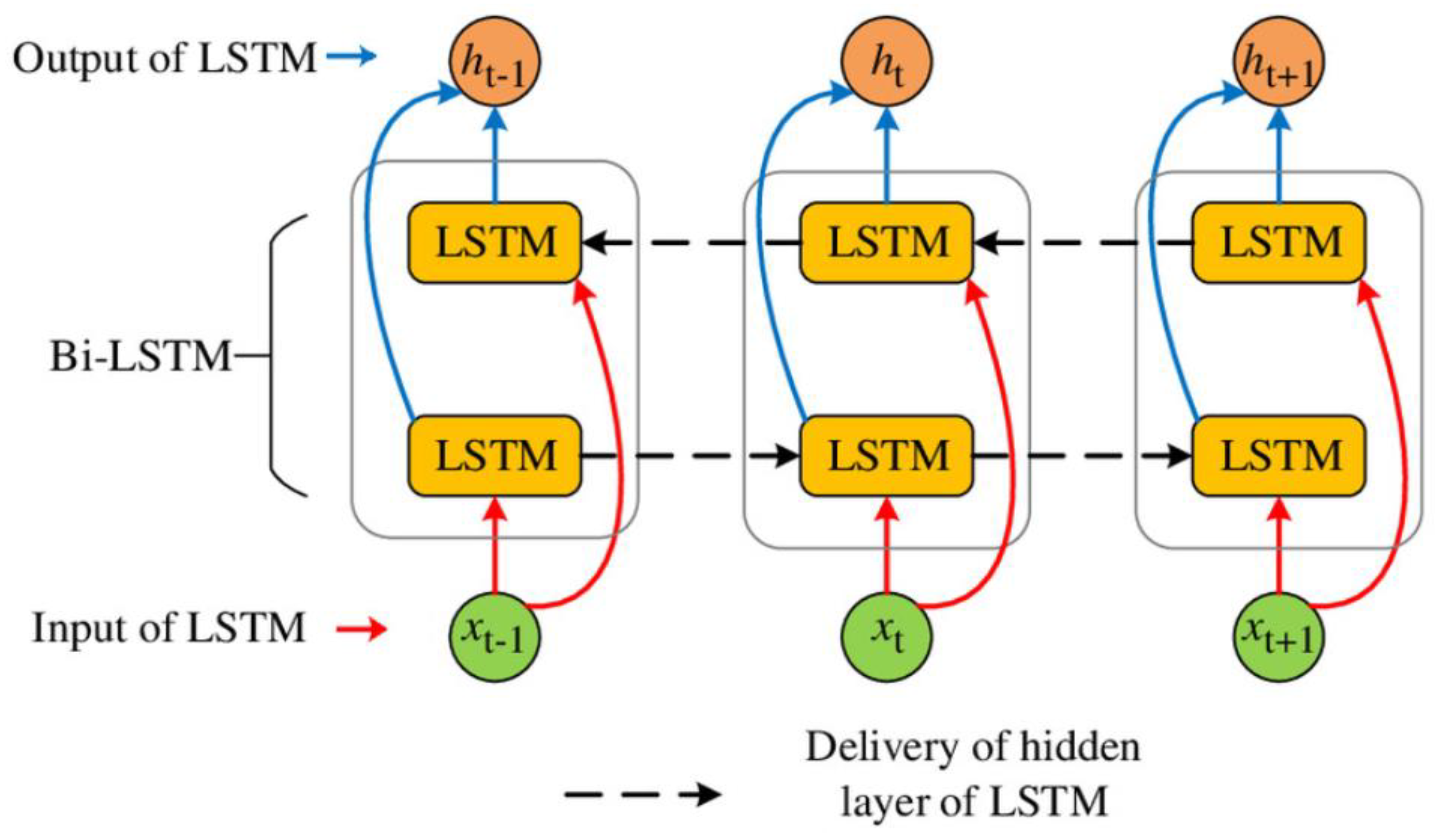
The Bi-LSTM architecture used in this study is shown in Figure 5. Where the LSTM model has only a hidden layer and it predicts output based on previous information, the Bi-LSTM model predicts based on the previous and subsequent data points. The well data contextual in nature are sequential and can be used as bidirectional during the entire training process. The hyperparameters are the same as the LSTM model mentioned above.

2.3. Processing of Data Set

The log data of the Permian Basin for the three wells studied in the work are numbered from P1 to P3. Out of all unconventional formations in the USA, Permian Basin is the most prolific hydrocarbon field that encompasses an area exceeding 86 thousand square miles in West Texas. The well depth found in this study ranges from 3000 to 12,000 feet. The well location and the lithologic characteristics are presented in Table 1.
During the processing of the data, depth-wise acoustic data were recorded with other logs. During the initial inspection of the raw, all the outliers were removed manually from the data. The data source for this study is the Railroad Commission (RRC), Texas.
To predict acoustic velocity, for all three wells, the data points used are described in Table 2, Table 3 and Table 4. To construct the model, a 75:25 ratio is used for training and testing the data. About 3500 data points from three selected wells were made unseen from RF and Bi-LSTM models and utilized later to validate. Each depth point has a total of six log parameters utilized as input and the DTS value targeted an output.
Table 2, Table 3 and Table 4 presented the statistical parameters of the dataset used to construct the models. The logging inputs below were obtained from Permian Basin wells and used in constructing this model:
  • Depth, (D) in ft
  • Porosity (POR) in %
  • Bulk density, (RHOB) in g/cm3
  • Compressional travel time (DTC) in µsec/ft
  • Gamma Ray (GR), in API
  • Formation Resistivity (RT) in Ω-m
To avoid overfitting, AI algorithms employed have an early stopping nature. The losses during training and validation events are assessed at each iteration, which is shown in Figure 6 for three wells.
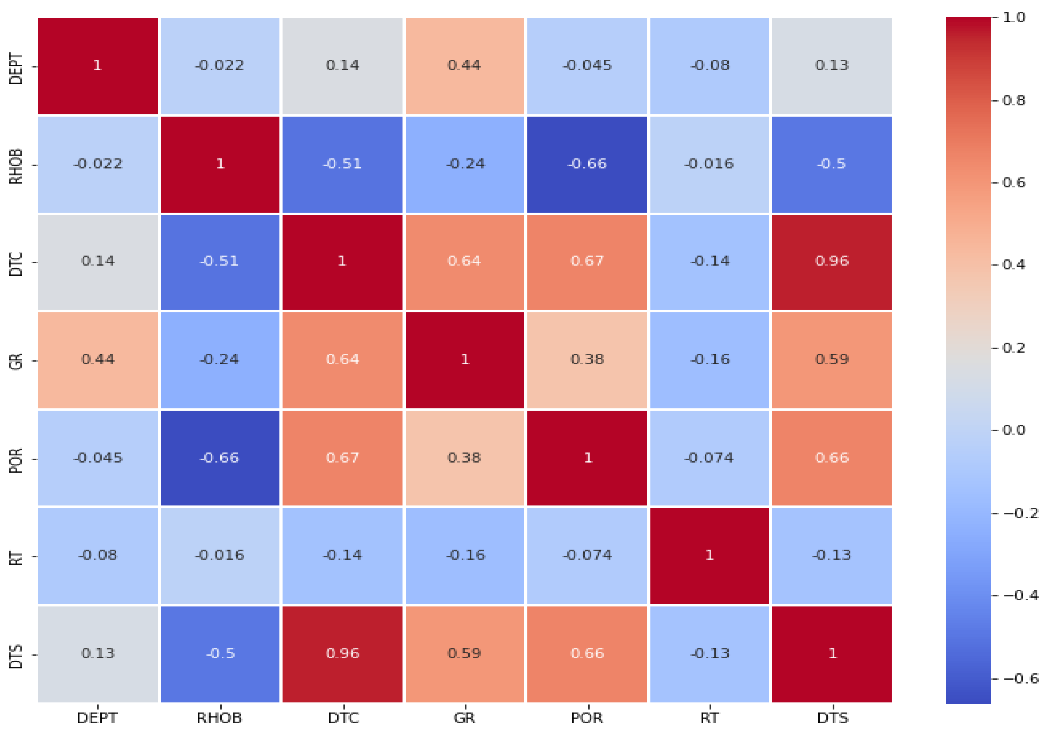
The correlation matrix from the initial input data is shown in Figure 7 and Figure 8 for single-well and grouped-well cases respectively. These heatmaps show how each feature is correlated with other well parameters. From Figure 7 and Figure 8, it is evident that all input parameters are positively correlated with each other, except for RT and RHOB values. This inconsistency more likely happened due to the regional difference and bad quality of the data obtained from the publicly shared domain, RRC. The parameters RT and RHOB are negatively or weakly correlated, as shown in the heatmap, which impacted the predictions made for both methods.

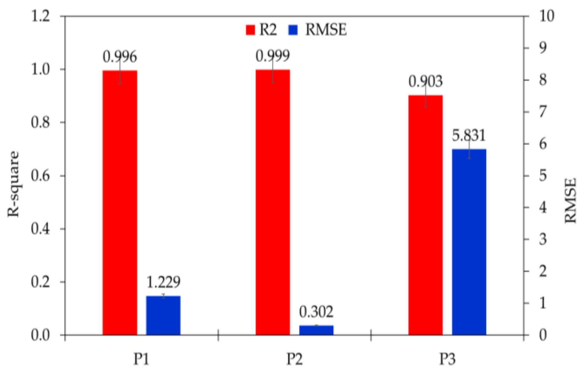
2.4. Performance Evaluation

This study presented an open-source Python-based Keras machine learning and deep learning application. Two statistical parameters were employed to compute and measure the target and estimated value, accuracy (R2) and root mean square error (RMSE) [49]. These parameters can be expressed by Equations (1) and (2):
R 2 = 1 i n ( y i f i ) 2 i n ( y i y ^ ) 2
where y i is the original value; predicted value is f i , and y ^ is the arithmetic average of all original values.
RMSE = 1 n i = 1 n ( y i     f i ) 2

3. Results and Analysis

3.1. Single-Well Prediction

In this prediction case, 75% of the data is used for training and the remaining 25% for testing. The input logs contain the depth-wise DTC, PHI, RHOB, GR, and RT. The output is shear wave slowness (DTS).
The R2 and RMSE of three wells predicted by these algorithms are presented in Table 5. P2 well achieves the best model performance predicted by RF algorithms with an R2 value of 99.90% and an error of less than 1% which is shown in Figure 9. Figure 10 shows the single well prediction using Bi-LSTM. Well P1 performs best of all three well using DL with an accuracy of 93.6%. In deep neural networks, Bi-LSTM exhibits lower accuracy compared to RF.
Figure 11 indicates the average model evaluation using both RF and Bi-LSTM for the single well case. The result shows that the highest accuracy obtained is 96.6% for the P1 well. Though RF and Bi-LSTM performed dissimilar for each well, the calculated average of both AI models’ predictions yielded a safe and realistic prediction, as shown in Figure 11. The average error obtained for the single-well prediction is below 7%.
The single-well DTS prediction results for all three wells are demonstrated in Figure 12. Results obtained using both RF and Bi-LSTM show a promising prediction with an excellent match of the predicted result with the original.

3.2. Cross-Well Predictions

During the single-well prediction, the RF algorithm performed superior compared to the Bi-LSTM model. Therefore, to enhance the model performance, the grouped well prediction was made employing both the RF and Bi-LSTM model. Overall evaluation, including individual well R2, RMSE, and the average for cross-well DTS prediction, is illustrated in Table 6.
Figure 13 shows that the P2 well demonstrates the best performance among all three wells for a cross-well prediction using the Bi-LSTM model exhibiting an accuracy value of 96.0% and an error of less than 5%. Figure 14 shows the cross-well prediction using Bi-LSTM. #P1 performs best of all three well using the RF algorithm with an accuracy of 93.8%. Deep neural network, Bi-LSTM exhibits better accuracy compared to RF except for the P3 well.
Figure 15 shows the evaluation of the average model prediction for the single well case. The results point out that the highest average accuracy was found at 94.10% for the P2 well. The grouped-well prediction yielded an average error below 7%. Both RF and Bi-LSTM performed closer for each well for cross-well prediction, but the calculated average of both models yielded a representative prediction.
Five-fold cross-validation was used to evaluate the model. In each stage of iteration, a total of two wells were used to train the model, and the remaining third well was used to model testing and DTC prediction. Finally, the arithmetic average was calculated and reported for both R2 and RMSE. The DTS prediction results for grouped well are demonstrated in Figure 16 for all three wells. This prediction was successfully tested blindly. While training the model, the predicted data were withdrawn completely from the training datasets.

3.3. Model Validation

The RF and Bi-LSTM model predicted results are validated by original DTS values. To serve as blind validation, original DTS values from the training dataset have been eliminated, thus boosting confidence in model performance. The contrast shows a great match between predicted and actual log data. The prediction results using the Bi-LSTM model for three wells are shown in Figure 17 below.

3.4. Estimation of Geomechanical Parameters

After blind validation and based on new prediction results, key elastic properties for the P1 well are calculated (Figure 18) using the following equation [55,56,57]. Overburden pressure is calculated using depth correlation, and pore pressure is assumed at 0.65 times the vertical depth.
Young s   Modulus ,   E = ρ b V s 2 ( 3 V p 2 4 V s 2 V p 2 V s 2 )
Poisson s   Ratio ,   υ = 1 2 ( V p 2 2 V s 2 V p 2 V s 2 )
Horizontal   Stress ,   σ m i n = υ ( 1 υ )   ( σ v P p )   +   P p

4. Discussions

The data analyzed in this work were received from the public domain, RRC [58], where obtained data quality was relatively poor for some wells. This impacted the prediction performance in the current study. Consequently, long steps were taken to perform the hyperparameter tuning of the data. During data processing, missing data were filled immediately before the data point of specific features. The average computational times are given in Table 7. Time is a variable here since data points are different for each well. The resistivity value (RT) obtained from the deep induction log shows very skewness and abnormal statistical distribution indicating poor quality of the recorded data. The input RT significantly impacted the prediction as indicated in the correlation matrix illustrated in the heatmap in Figure 7 and Figure 8.
A deep neural network might provide better prediction results but requires a time-consuming route for constructing and validating the model. Compared to the DL, RF requires relatively a smaller amount of time for testing and training the model [59]. It is noted that the deep neural network is best for large sets of data. The size of the numeric data point used in this study is within 11,000–15,000 for which the RF model exhibits efficiency. Therefore, choosing the model based on the data size is crucial for the efficient use of these algorithms.

5. Conclusions

In this study, Bi-LSTM and RF models have been presented to predict the acoustic properties and estimate the geomechanical of the Permian Basin wells. The key outcomes obtained are as follows:
  • The single-well prediction method using the RF algorithm provided the highest accuracy of 99.90% whereas in Bi-LSTM gives 93.60%. The maximum average accuracy reported for a single well is 96.60%. The average error found for both single-well prediction and grouped well method is below 7%.
  • The best accuracy for a grouped well prediction was achieved employing Bi-LSTM is 96.01% whereas the RF model provided 93.80%. The grouped well prediction yielded a maximum accuracy of 94.10%.
  • Bi-LSTM shows better accuracy for P2 well in grouped prediction while the RF algorithm achieved superior predictions for a single well, grouped well, known, and completely unknown DTS data sets.
  • To predict the geomechanical properties of shale formations where inadequate or missing datasets are present, AI can be an efficient alternative to retrieve missing or unknown information.
  • Both RF and Bi-LSTM predictions show an excellent match with known and completely unknown well-log datasets, demonstrating the strength of the prediction made in this work.
The key outcome yielded from this study could be a predictive tool for increasing hydrocarbon recovery from unconventional reservoirs. The output will be beneficial in assessing the dynamic and static elastic characteristics which are crucial for planning an effective and efficient completion plan with reduced cost.

Author Contributions

Conceptualization, F.N.; methodology, F.N. and S.M.A.; validation, F.N.; formal analysis, F.N. and S.M.A.; software, S.M.A.; investigation, F.N., H.R.D., G.A. and E.A.; resources, F.N.; data curation, G.A., E.A. and S.M.A.; writing—original draft preparation, F.N.; writing—review and editing F.N., S.M.A. and D.G.; supervision, F.N.; project administration, F.N.; funding acquisition, F.N. All authors have read and agreed to the published version of the manuscript.

Funding

This research received no external funding.

Institutional Review Board Statement

Not applicable.

Informed Consent Statement

Not applicable.

Data Availability Statement

The data presented in this study are available on request from the corresponding author.

Acknowledgments

The authors thank Texas A&M International University for supporting the necessary equipment for this work with a start-up research fund and accelerating undergraduate research through a university research grant (URG).

Conflicts of Interest

The authors declare no conflict of interest.

References

  1. Eshkalak, M.O.; Mohaghegh, S.D.; Esmaili, S. Geomechanical properties of unconventional shale reservoirs. J. Pet. Eng. 2014, 2014, 961641. [Google Scholar] [CrossRef] [Green Version]
  2. Greenberg, M.L.; Castagna, J.P. Shear-Wave Velocity Estimation in Porous Rocks: Theoretical Formulation, Preliminary Verification and applications1. Geophys. Prospect. 1992, 40, 195–209. [Google Scholar] [CrossRef]
  3. Ruse, C.M.; Mokhtari, M. Characterization of Elastic Mechanical Properties of Tuscaloosa Marine Shale from Well Logs Using the Vertical Transversely Isotropic Model. Interpretation 2020, 8, T1023–T1036. [Google Scholar] [CrossRef]
  4. Chang, C.; Zoback, M.D.; Khaksar, A. Empirical Relations between Rock Strength and Physical Properties in Sedimentary Rocks. J. Pet. Sci. Eng. 2006, 51, 223–237. [Google Scholar] [CrossRef]
  5. Asoodeh, M.; Bagheripour, P. Prediction of Compressional, Shear, and Stoneley Wave Velocities from Conventional Well Log Data Using a Committee Machine with Intelligent Systems. Rock Mech. Rock Eng. 2011, 45, 45–63. [Google Scholar] [CrossRef]
  6. Onalo, D.; Adedigba, S.; Khan, F.; James, L.A.; Butt, S. Data Driven Model for Sonic Well Log Prediction. J. Pet. Sci. Eng. 2018, 170, 1022–1037. [Google Scholar] [CrossRef]
  7. Hossain, Z.; Mukerji, T.; Fabricius, I.L. VP-Vs Relationship and Amplitude Variation with Offset Modelling of Glauconitic Greensand‡. Geophys. Prospect. 2011, 60, 117–137. [Google Scholar] [CrossRef]
  8. Castagna, J.P.; Batzle, M.L.; Eastwood, R.L. Relationships between Compressional-Wave and Shear-Wave Velocities in Clastic Silicate Rocks. Geophysics 1985, 50, 571–581. [Google Scholar] [CrossRef]
  9. Chu, Z.; Lu, B. A new method for estimating formation shear wave velocity. Well Logging Technol. 1995, 19, 313–318. [Google Scholar]
  10. Potter, C.C.; Foltinek, D.S. Formation elastic parameters by deriving S-wave velocity logs. Consort. Res. Elastic 1997, 9, 10–23. [Google Scholar]
  11. Brocher, T.M. Empirical Relations between Elastic Wavespeeds and Density in the Earth’s Crust. Bull. Seismol. Soc. Am. 2005, 95, 2081–2092. [Google Scholar] [CrossRef]
  12. Bukar, I.; Adamu, M.B.; Hassan, U. A Machine Learning Approach to Shear Sonic Log Prediction. In Proceedings of the SPE Nigeria Annual International Conference and Exhibition, Lagos, Nigeria, 5–7 August 2019. [Google Scholar] [CrossRef]
  13. Hanoon, M.S.; Ahmed, A.N.; Zaini, N.; Razzaq, A.; Kumar, P.; Sherif, M.; Sefelnasr, A.; El-Shafie, A. Developing Machine Learning Algorithms for Meteorological Temperature and Humidity Forecasting at Terengganu State in Malaysia. Nat. Sci. Rep. 2021, 11, 18935. [Google Scholar] [CrossRef] [PubMed]
  14. Osman, A.I.; Ahmed, A.N.; Huang, Y.F.; Kumar, P.; Birima, A.H.; Sherif, M.; Sefelnasr, A.; Ebraheemand, A.A.; El-Shafie, A. Past, Present, and Perspective Methodology for Groundwater Modeling-Based Machine Learning Approaches. Arch. Comput. Methods Eng. 2022, 29, 3843–3859. [Google Scholar] [CrossRef]
  15. Zerrouki, A.A.; Aïfa, T.; Baddari, K. Prediction of Natural Fracture Porosity from Well Log Data by Means of Fuzzy Ranking and an Artificial Neural Network in Hassi Messaoud Oil Field, Algeria. J. Pet. Sci. Eng. 2014, 115, 78–89. [Google Scholar] [CrossRef]
  16. Wood, D.A. Predicting Porosity, Permeability and Water Saturation Applying an Optimized Nearest-Neighbour, Machine-Learning and Data-Mining Network of Well-Log Data. J. Pet. Sci. Eng. 2020, 184, 106587. [Google Scholar] [CrossRef]
  17. Al Khalifah, H.; Glover, P.W.J.; Lorinczi, P. Permeability Prediction and Diagenesis in Tight Carbonates Using Machine Learning Techniques. Mar. Pet. Geol. 2020, 112, 104096. [Google Scholar] [CrossRef]
  18. Shokooh Saljooghi, B.; Hezarkhani, A. A New Approach to Improve Permeability Prediction of Petroleum Reservoirs Using Neural Network Adaptive Wavelet (Wavenet). J. Pet. Sci. Eng. 2015, 133, 851–861. [Google Scholar] [CrossRef]
  19. Alloush, R.M.; Elkatatny, S.M.; Mahmoud, M.A.; Moussa, T.M.; Ali, A.Z.; Abdulraheem, A. Estimation of geomechanical failure parameters from well logs using artificial intelligence techniques. In Proceedings of the SPE Kuwait Oil and Gas Show and Conference, Kuwait City, Kuwait, 13 October 2017. [Google Scholar] [CrossRef]
  20. Tariq, Z.; Elkatatny, S.; Mahmoud, M.; Ali, A.Z.; Abdulraheem, A. A new technique to develop rock strength correlation using artificial intelligence tools. In Proceedings of the SPE Reservoir Characterization and Simulation Conference and Exhibition, Abu Dhabi, United Arab Emirates, 14 May 2017. [Google Scholar] [CrossRef]
  21. Elkatatny, S.; Tariq, Z.; Mahmoud, M.; Abdulazeez, A.; Mohamed, I.M. Application of artificial intelligence techniques to determine sonic time from well logs. In Proceedings of the 50th U.S. Rock Mechanics/Geomechanics Symposium, Houston, TX, USA, 26–29 June 2016. [Google Scholar]
  22. Ahmadi, M.A.; Pournik, M.; Shadizadeh, S.R. Toward Connectionist Model for Predicting Bubble Point Pressure of Crude Oils: Application of Artificial Intelligence. Petroleum 2015, 1, 307–317. [Google Scholar] [CrossRef] [Green Version]
  23. Alakbari, F.S.; Elkatatny, S.; Baarimah, S.O. Prediction of bubble point pressure using artificial intelligence AI techniques. In Proceedings of the SPE Middle East Artificial Lift Conference and Exhibition, Manama, Bahrain, 30 November–1 December 2016. [Google Scholar] [CrossRef]
  24. Wood, D.A.; Choubineh, A. Transparent Open-Box Learning Network and Artificial Neural Network Predictions of Bubble-Point Pressure Compared. Petroleum 2020, 6, 375–384. [Google Scholar] [CrossRef]
  25. Mahdiani, M.R.; Norouzi, M. A New Heuristic Model for Estimating the Oil Formation Volume Factor. Petroleum 2018, 4, 300–308. [Google Scholar] [CrossRef]
  26. Oloso, M.A.; Hassan, M.G.; Bader-El-Den, M.B.; Buick, J.M. Hybrid Functional Networks for Oil Reservoir PVT Characterization. Expert Syst. Appl. 2017, 87, 363–369. [Google Scholar] [CrossRef] [Green Version]
  27. Elkatatny, S.; Moussa, T.; Abdulraheem, A.; Mahmoud, M. A Self-Adaptive Artificial Intelligence Technique to Predict Oil Pressure Volume Temperature Properties. Energies 2018, 11, 3490. [Google Scholar] [CrossRef] [Green Version]
  28. Ahmed, A.; Ali, A.; Elkatatny, S.; Abdulraheem, A. New Artificial Neural Networks Model for Predicting Rate of Penetration in Deep Shale Formation. Sustainability 2019, 11, 6527. [Google Scholar] [CrossRef] [Green Version]
  29. Al-AbdulJabbar, A.; Elkatatny, S.; Abdulhamid Mahmoud, A.; Moussa, T.; Al-Shehri, D.; Abughaban, M.; Al-Yami, A. Prediction of the Rate of Penetration While Drilling Horizontal Carbonate Reservoirs Using the Self-Adaptive Artificial Neural Networks Technique. Sustainability 2020, 12, 1376. [Google Scholar] [CrossRef] [Green Version]
  30. Elkatatny, S. Real-Time Prediction of Rate of Penetration in S-Shape Well Profile Using Artificial Intelligence Models. Sensors 2020, 20, 3506. [Google Scholar] [CrossRef]
  31. Hassan, A.; Al-Majed, A.; Mahmoud, M.; Elkatatny, S.; Abdulraheem, A. Improved Predictions in Oil Operations Using Artificial Intelligent Techniques. In Proceedings of the SPE Middle East Oil Gas Show Conference, Manama, Bahrain, 18–21 March 2019. [Google Scholar] [CrossRef]
  32. Abdelgawad, K.Z.; Elzenary, M.; Elkatatny, S.; Mahmoud, M.; Abdulraheem, A.; Patil, S. New Approach to Evaluate the Equivalent Circulating Density (ECD) Using Artificial Intelligence Techniques. J. Pet. Explor. Prod. Technol. 2018, 9, 1569–1578. [Google Scholar] [CrossRef] [Green Version]
  33. Siddig, O.; Gamal, H.; Elkatatny, S.; Abdulraheem, A. Real-Time Prediction of Poisson’s Ratio from Drilling Parameters Using Machine Learning Tools. Sci. Rep. 2021, 11, 12611. [Google Scholar] [CrossRef]
  34. Abdelgawad, K.; Elkatatny, S.; Moussa, T.; Mahmoud, M.; Patil, S. Real-Time Determination of Rheological Properties of Spud Drilling Fluids Using a Hybrid Artificial Intelligence Technique. J. Energy Resour. Technol. 2019, 141, 756–765. [Google Scholar] [CrossRef]
  35. Al-azani, K.; Elkatatny, S.; Abdulraheem, A.; Mahmoud, M.; Al-Shehri, D. Real-time prediction of the rheological properties of oil-based drilling fluids using artificial neural networks. In Proceedings of the SPE Kingdom of Saudi Arabia Annual Technical Symposium and Exhibition, Dammam, Saudi Arabia, 23–26 April 2018. [Google Scholar] [CrossRef]
  36. Elkatatny, S. Real-Time Prediction of the Rheological Properties of Water-Based Drill-in Fluid Using Artificial Neural Networks. Sustainability 2019, 11, 5008. [Google Scholar] [CrossRef] [Green Version]
  37. Rajabi, M.; Bohloli, B.; Gholampour Ahangar, E. Intelligent Approaches for Prediction of Compressional, Shear and Stoneley Wave Velocities from Conventional Well Log Data: A Case Study from the Sarvak Carbonate Reservoir in the Abadan Plain (Southwestern Iran). Comput. Geosci. 2010, 36, 647–664. [Google Scholar] [CrossRef]
  38. Rajabi, M.; Tingay, M. Applications of Intelligent Systems in Petroleum Geomechanics—Prediction of Geomechanical Properties in Different Types of Sedimentary Rocks. In International EAGE Workshop on Geomechanics and Energy; European Association of Geoscientists & Engineers: Houten, The Netherlands, 2013; p. cp-369. [Google Scholar] [CrossRef]
  39. Maleki, S.; Moradzadeh, A.; Riabi, R.G.; Gholami, R.; Sadeghzadeh, F. Prediction of Shear Wave Velocity Using Empirical Correlations and Artificial Intelligence Methods. NRIAG J. Astron. Geophys. 2014, 3, 70–81. [Google Scholar] [CrossRef] [Green Version]
  40. Zoveidavianpoor, M. A Comparative Study of Artificial Neural Network and Adaptive Neurofuzzy Inference System for Prediction of Compressional Wave Velocity. Neural Comput. Appl. 2014, 25, 1169–1176. [Google Scholar] [CrossRef]
  41. Lorentzen, M.; Bredesen, K.; Mosegaard, K.; Nielsen, L. Estimation of shear sonic logs in the heterogeneous and fractured Lower Cretaceous of the Danish North Sea using supervised learning. Geophys. Prospect. 2022, 70, 1410–1431. [Google Scholar] [CrossRef]
  42. Aleardi, M. Seismic Velocity Estimation from Well Log Data with Genetic Algorithms in Comparison to Neural Networks and Multilinear Approaches. J. Appl. Geophys. 2015, 117, 13–22. [Google Scholar] [CrossRef]
  43. Rezaee, M.R.; Kadkhodaie Ilkhchi, A.; Barabadi, A. Prediction of Shear Wave Velocity from Petrophysical Data Utilizing Intelligent Systems: An Example from a Sandstone Reservoir of Carnarvon Basin, Australia. J. Pet. Sci. Eng. 2007, 55, 201–212. [Google Scholar] [CrossRef]
  44. Cranganu, C.; Bautu, E. Using Gene Expression Programming to Estimate Sonic Log Distributions Based on the Natural Gamma Ray and Deep Resistivity Logs: A Case Study from the Anadarko Basin, Oklahoma. J. Pet. Sci. Eng. 2010, 70, 243–255. [Google Scholar] [CrossRef]
  45. Zoveidavianpoor, M.; Samsuri, A.; Shadizadeh, S.R. Prediction of Compressional Wave Velocity by an Artificial Neural Network Using Some Conventional Well Logs in a Carbonate Reservoir. J. Geophys. Eng. 2013, 10. [Google Scholar] [CrossRef]
  46. Akhundi, H.; Ghafoori, M.; Lashkaripour, G.-R. Prediction of Shear Wave Velocity Using Artificial Neural Network Technique, Multiple Regression and Petrophysical Data: A Case Study in Asmari Reservoir (SW Iran). Open J. Geol. 2014, 4, 303–313. [Google Scholar] [CrossRef] [Green Version]
  47. Song, L.; Liu, Z.; Li, C.; Ning, C.; Hu, Y.; Wang, Y.; Hong, F.; Tang, W.; Zhuang, Y.; Zhang, R.; et al. Prediction and Analysis of Geomechanical Properties of Jimusaer Shale Using a Machine Learning Approach. In Proceedings of the SPWLA 62nd Annual Online Symposium Transactions, Online, 17–20 May 2021. [Google Scholar] [CrossRef]
  48. Enverus. 2022. Available online: https://www.enverus.com (accessed on 10 September 2022).
  49. Nath, F.; Murillo, K.; Asish, S.M.; Ganta, D.; Limon, V.; Aguirre, E.; Aguirre, G.; Debi, H.R.; Perez, J.L.; Netro, C.; et al. Prediction and Analysis of Geomechanical Properties Using Deep Learning: A Permian Basin Case Study. Paper Presented at the SPE/AAPG/SEG Unconventional Resources Technology Conference, Houston, TX, USA, 20 June 2022. [Google Scholar] [CrossRef]
  50. Ramiro-Ramirez, S.; Bhandari, A.R.; Flemings, P.B.; Robert, R.M. Porosity and Permeability Heterogeneity in the Upper Wolfcamp, Delaware Basin, West Texas: Implications for Production. Paper Presented at the SPE/AAPG/SEG Unconventional Resources Technology Conference, Virtual, 20–22 July 2020; 2020. [Google Scholar] [CrossRef]
  51. Chen, Y.; Zhang, D. Physics-Constrained Deep Learning of Geomechanical Logs. IEEE Trans. Geosci. Remote Sens. 2020, 58, 5932–5943. [Google Scholar] [CrossRef]
  52. Hochreiter, S.; Schmidhuber, J. Long Short-Term Memory. Neural Comput. 1997, 9, 1735–1780. [Google Scholar] [CrossRef]
  53. Zaremba, W.; Sutskever, I.; Vinyals, O. Recurrent neural network regularization. arXiv 2014, arXiv:1409.2329. [Google Scholar]
  54. King, M.S. Static and dynamic elastic moduli of rocks under pressure. In Proceedings of the 11th U.S. Symposium on Rock Mechanics (USRMS), Berkeley, CA, USA, 16–19 June 1969. ARMA-69-0329. [Google Scholar]
  55. Ogunkunle, T.F.; Okoro, E.E.; Rotimi, O.J.; Igbinedion, P.; Olatunji, D.I. Artificial Intelligence Model for Predicting Geomechanical Characteristics Using Easy-to-Acquire Offset Logs without Deploying Logging Tools. Petroleum 2022, 8, 192–203. [Google Scholar] [CrossRef]
  56. Abdulraheem, A.; Ahmed, M.; Vantala, A.; Parvez, T. Prediction of rock mechanical parameters for hydrocarbon reservoirs using different artificial intelligence techniques. In Proceedings of the SPE Saudi Arabia Section Technical Symposium, Al-Khobar, Saudi Arabia, 11 May 2009. [Google Scholar] [CrossRef]
  57. Al-Anazi, B.D.; Al-Garni, M.T.; Muffareh, T.; Al-Mushigeh, I. Prediction of Poisson’s Ratio and Young’s Modulus for Hydrocarbon Reservoirs Using Alternating Conditional Expectation Algorithm. In Proceedings of the SPE Middle East Oil and Gas Show and Conference, Manama, Bahrain, 9 September 2011. [Google Scholar] [CrossRef]
  58. RRC. 2022. Available online: www.rrc.texas.gov (accessed on 25 April 2022).
  59. Essam, Y.; Ahmed, A.N.; Ramli, R.; Chau, K.-W.; Idris Ibrahim, M.S.; Sherif, M.; Sefelnasr, A.; El-Shafie, A. Investigating Photovoltaic Solar Power Output Forecasting Using Machine Learning Algorithms. Eng. Appl. Comput. Fluid Mech. 2022, 16, 2002–2034. [Google Scholar] [CrossRef]
Figure 1. The geographic region of the Permian Basin, West Texas. The study area is in the Reeves county of Delaware Basin, and wells from Upton and Glasscock counties of Midland Basin (green-red star). Midland and Delaware basin stratigraphy is adapted from Ramiro-Ramirez et al. [50].
Energies 15 08752 g001
Figure 4. Architecture of Artificial Neural Network.
Energies 15 08752 g004
Figure 5. Architecture of Deep Neural Network (Bi-LSTM) (adapted from Zaremba et al. [53]).
Energies 15 08752 g005
Figure 6. Loss vs. Epoch on validation data during training for different wells.
Energies 15 08752 g006
Figure 7. Heat map for a single well.
Energies 15 08752 g007
Figure 8. Heat map for cross well.
Energies 15 08752 g008
Figure 9. Single-well prediction using RF.
Energies 15 08752 g009
Figure 10. Single-well prediction using Bi-LSTM.
Energies 15 08752 g010
Figure 11. Average R2 and RMSE for single-well prediction.
Energies 15 08752 g011
Figure 12. Actual vs. predicted DTS value from single well prediction using RF and Bi-LSTM model.
Energies 15 08752 g012aEnergies 15 08752 g012b
Figure 13. Cross-well prediction using RF.
Energies 15 08752 g013
Figure 14. Cross-well prediction using Bi-LSTM.
Energies 15 08752 g014
Figure 15. Average R2 and RMSE for cross-well prediction.
Energies 15 08752 g015
Figure 16. Actual vs. predicted DTS value from cross-well prediction using Random Forest and Bi-LSTM.
Energies 15 08752 g016
Figure 17. Validation for (a) P1 well, (b) P2 well (c) P3 well.
Energies 15 08752 g017
Figure 18. Estimation of geomechanical properties from predicted DTS for P1 well.
Energies 15 08752 g018
Table 1. Well location and the lithologic characteristics.
WellCounty BasinLithological Characteristics
P1GlasscockMidlandClastic-carbonate and shaly limestone
P2ReevesDelawareInterbedded sandstone with organic-rich siltstone
P3UptonMidlandLimestone interbedded with shale and sandstone
Table 2. Dataset information from P1 well (Total datapoint = 14,235).
DepthRHOBRTGRPORDTC
Minimum32212.3370.1676.3320.001241.897
Maximum103822.9421065.73570.6390.21896.009
Mean6791.932.661530.8257.1960.04561.712
Std. Dev2060.980.080178.2243.2340.03111.16
Table 3. Dataset information from P2 well (Total = 11,009).
DepthRHOBRTGRPORDTC
Minimum251.51.4750.01132.110.000144.93
Maximum58223.6251987.3794.8850.7554154.414
Mean3034.172.5490705.4528.4170.116564.03
Std. Dev1605.270.3561183.9816.6970.08712.3916
Table 4. Dataset information from P3 well (Total = 15,025).
DepthRHOBRTGRPORDTC
Minimum59902.33556.303212.10920.000255.12
Maximum87712.74091496.5239.4960.322593.197
Mean7392.712.5494184.0786.2830.146768.134
Std. Dev800.010.056615.9428.670.05328.3736
Table 5. R2 and RMSE for single well DTS prediction.
AI ModelRandom ForestBi-LSTMAverage
WellsR2RMSER2RMSER2RMSE
P10.9961.2290.9365.6200.9663.424
P20.9990.3020.8812.9300.9401.616
P30.9035.8310.8097.6000.8566.716
Table 6. R2 and RMSE for cross-well prediction.
AI ModelRF ModelBi-LSTMAverage
WellsR2RMSER2RMSER2RMSE
P10.9384.9640.9215.610.9375.012
P20.9305.9220.9604.510.9415.431
P30.8525.9070.7807.860.8206.384
Table 7. Average computational time.
ModeRandom ForestBi-LSTM
Single well~1 s1–2 min
Cross well15–20 s15–30 min
Publisher’s Note: MDPI stays neutral with regard to jurisdictional claims in published maps and institutional affiliations.

