1. Introduction
With the development of near space flight and transport technology, hypersonic flight technology is proposed [
1]. Compared with traditional low-speed and supersonic aircraft, hypersonic aircraft have the characteristics of higher speed, lower interference, and longer voyage [
2]. The optical dome is a vital part of hypersonic aircraft and must withstand extremely high temperatures and pass through electromagnetic waves and infrared signals of various bands [
3]. However, due to aerodynamic heating, a large amount of heat flow is transmitted to the optical dome; this increases the internal temperature and endangers the electronic equipment inside the optical dome [
3]. The aerodynamic heating is strongest near the optical dome, and the heat distribution of precision instruments inside the optical dome is closely related to the optical dome temperature distribution [
4]. Therefore, it is necessary to study the aerodynamic heat transfer of the optical dome for hypersonic aircraft.
Many countries are conducting extensive research on hypersonic technologies, especially the development of hypersonic aircraft for use in near space. Hamilton [
5] proposed an algorithm for the aerodynamic heating on the windward side of the space shuttle to predict the heat flux density in the windward surface flow and turbulent region. The results obtained using the algorithm were consistent with the wind tunnel test and actual flight test results. Davis [
6] simplified the Navier–Stokes equation and obtained the viscous shock layer equation by retaining the quadratic term of the Reynolds parameter in the Euler equation. When calculating the aerodynamic and thermal parameters of the flow region behind the shock wave, the calculation accuracy of this equation is higher than that of the boundary layer equation. Riley [
7] proposed an approximation algorithm for the convection heat transfer in the aerodynamic heat flow on the surface of hypersonic aircrafts under the assumption of ideal gas inviscid flow. This algorithm can be used to calculate the aerodynamic heat generated by different shapes and laminar turbulence. Lei et al. [
8] proposed a hybrid algorithm to calculate the aerodynamic heat of hypersonic aircraft and calculated the heat flow and temperature distribution. Experimental data demonstrated the effectiveness of this algorithm. By using the reference temperature method and semi-empirical formula, Che et al. [
9] calculated the aerodynamic heat of hypersonic aircraft at different stages and established the heat transfer equation by combining aerodynamic heating, thermal radiation on the aircraft surface, and heat conduction inside the aircraft shell. They found that the temperature of the aircraft dome changes with time. Xia et al. [
10] used the finite volume method and finite element method to simulate the coupling process between the high-speed flow and heat conduction in the blunt body; the obtained results were consistent with the wind tunnel test results.
In this study, a numerical simulation method for unsteady hypersonic aerodynamic heating and a fluid-thermal coupling effect is proposed. In addition, the aerodynamic heat transfer characteristics of a hypersonic aircraft optical dome are obtained.
5. Results and Discussion
We have studied the temperature and pressure of the aircraft optical dome during the whole flight. The flight time is from 20 s to 330 s. To simplify the analysis, we assume that the attack angle is 0°.
Figure 13 shows the change of aircraft flight altitude with time. The maximum flight altitude is approximately 60 km, and the aircraft enters the reentry section immediately after reaching the maximum altitude at about 160 s.
The flight velocity at different flight altitudes affects the aerodynamic heating of the aircraft. The flight velocity of the aircraft is shown in
Figure 14. The flight velocity rapidly increases to the hypersonic state at 20 s, and the maximum velocity of the aircraft reaches about 2500 m/s. Subsequently, the flight remains in a hypersonic state in a certain period. At around 300 s, the aircraft begins to decelerate from the hypersonic state, the velocity of the aircraft drops from 2000 m/s at 276 s to 500 m/s at 330 s.
Figure 15 shows the changes in the average temperature of the inner and outer walls of the optical dome with time. The wall temperature distribution exhibits an “M” shape, with two high-temperature cusps and one low-temperature cusp. At 70 s, the average temperature reaches the first peak of 1565 K. At 290 s, the average temperature reaches the second peak of 1560 K. There is a low-temperature cusp between the two peaks at 190 s, when the average temperature of the optical dome is 1130 K. The temperature increases rapidly before 70 s and reaches 1550 K at around 50 s. From 70 s to 290 s, the temperature firstly decreases and then increases, but the total change is within 450 K. It can be seen from
Figure 13 that the aircraft experiences lift-off and reentry processes during this period. From 290 s to the end, the temperature decreases rapidly, and the change rate of temperature is similar to that at the beginning of the flight.
Figure 16 shows the maximum temperature of the optical dome during the flight. The trend of the maximum temperature of the optical dome is similar to that of the average temperature distribution. The first peak (1660 K) of the maximum temperature appears at 70 s, and the second peak (1640 K) appears at 290 s. Between the two high-temperature cusps, a low-temperature cusp (1190 K) appears at 190 s. From the results shown in
Figure 15 and
Figure 16, it is found that the time when the average temperature is the highest overlaps with the time when the wall temperature is the highest. Due to the long flight duration, heat conduction inside the optical dome transfers the heat evenly, and the temperature gradient of the structure decreases correspondingly. The optical dome temperature changes continuously during the flight. When the temperature in one position is very high, the temperature in other positions also increases due to heat conduction. In addition, there is a fourth-power relationship between radiation effect and temperature. The radiation effect in high-temperature areas is stronger than that in low-temperature areas; this also balances the wall temperature distribution. Therefore, the maximum temperature and average temperature of the optical dome are related.
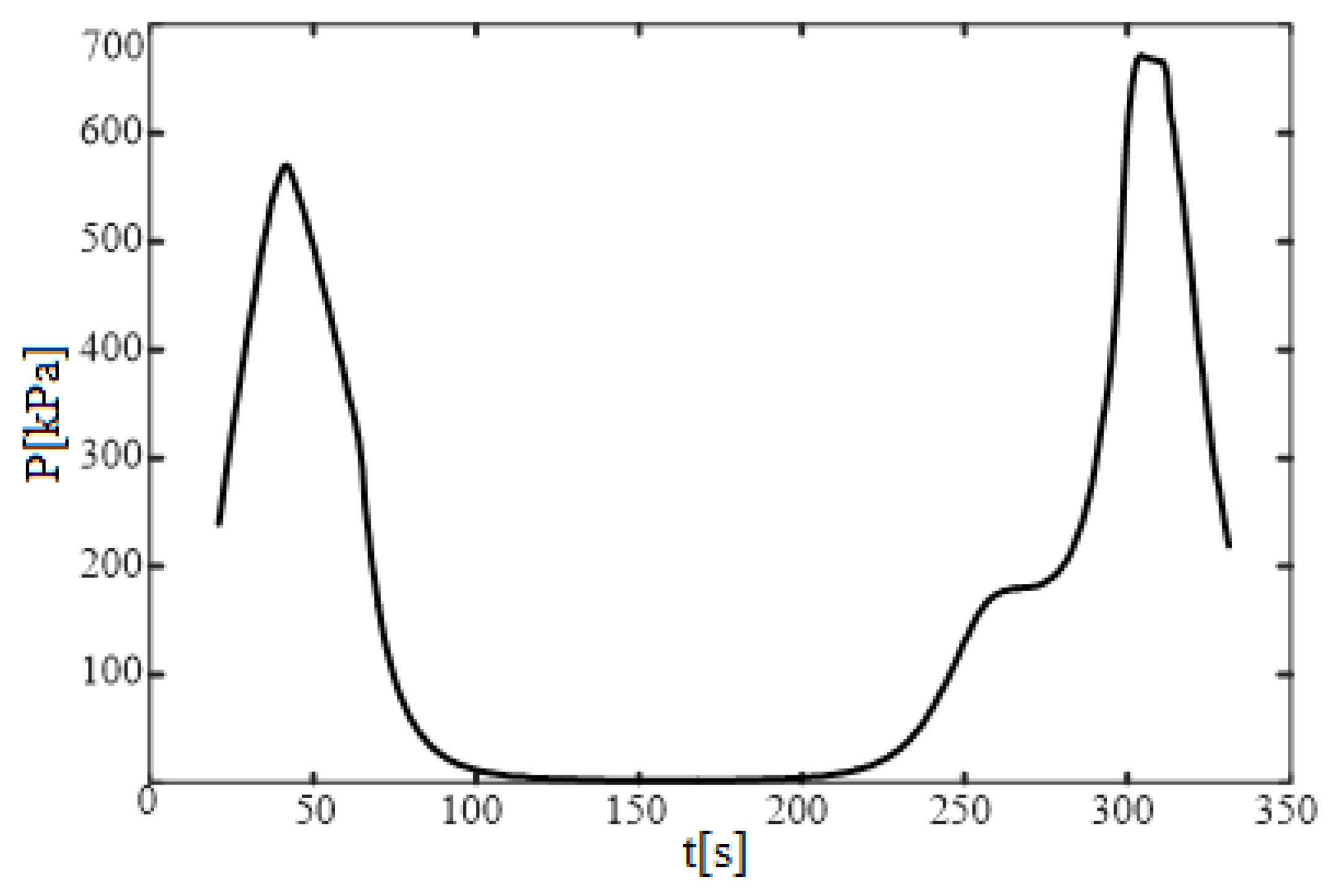
Figure 17 shows the maximum pressure on the outer wall of the optical dome with time during the flight. The wall pressure is high at both ends and low in the middle. The maximum pressure on the optical dome wall is below 700 kPa during the whole flight. The hypersonic wall pressure distribution is closely related to the inflow pressure and Mach number, and the inflow pressure is related to the flight altitude. Generally, the higher the flight altitude, the thinner the air and the lower the inflow pressure. At an altitude of 60 km, the atmospheric pressure is less than that of the horizontal plane. As shown in
Figure 17, the pressure on the optical dome wall firstly increases and then decreases. The rapid increase in the Mach number plays a major role in this process, and the decrease is caused by the decrease in the inflow pressure due to the change in the flight altitude. In the reentry phase, the pressure firstly increases and then decreases, which is contrary to the pressure change in the previous phase. Firstly, the pressure on the optical dome wall increases due to the altitude decrease and the inflow pressure increase. Then, the pressure on the optical dome wall decreases due to the sharp decrease in Mach number. Although the pressure on the optical dome wall varies greatly during the whole flight, the pressure magnitude is far below the maximum safety range of the optical dome. Therefore, the aerodynamic heat problem encountered in the aircraft is more serious and prominent than the problem of structure pressure.
According to the overall temperature and pressure changes of the optical dome, the whole flight can be divided into four periods for detailed analysis according to the “M” shape. The first time period is from 20 s to 70 s, the second period is from 70 s to 190 s, the third period is from 190 s to 290 s, and the fourth period is from 290 s to the end time of 330 s. The aerodynamic heat transfer characteristics of the optical dome are analyzed in combination with the variation of the inflow parameters such as flight altitude and the Mach number.
5.1. Analysis of Results in the First Period
Figure 18,
Figure 19,
Figure 20 and
Figure 21 show numerical results of the aircraft structure and the temperature field, the pressure of the external flow field, and temperature distribution of the optical dome structure at different time points in the first period (between 20 s and 70 s), respectively.
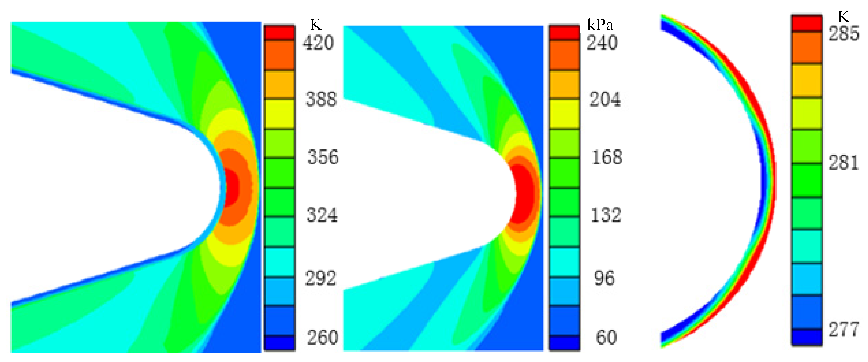
Figure 18 shows the results at 22 s when the flight altitude is approximately 3.5 km; the maximum temperature of the external flow field is around 420 K, and the temperature of the solid structure does not increase much compared with the inflow temperature. At this time, the flight velocity is less than Mach 2, the generated shock wave presents a large shock angle, and the parameters before and after the shock wave change only slightly. The maximum pressure near the optical dome is approximately 240 kPa and gradually decreases along the direction of fluid flow as the velocity increases. From the temperature distribution of the optical dome structure, shown on the right side of
Figure 18, the outer wall of the optical dome is heated up and conducts heat to the inside. However, because the aerodynamic heating time is relatively short, the aerodynamic heat intensity is not high when the Mach number is not large, and the overall temperature of the optical dome structure changes slightly.
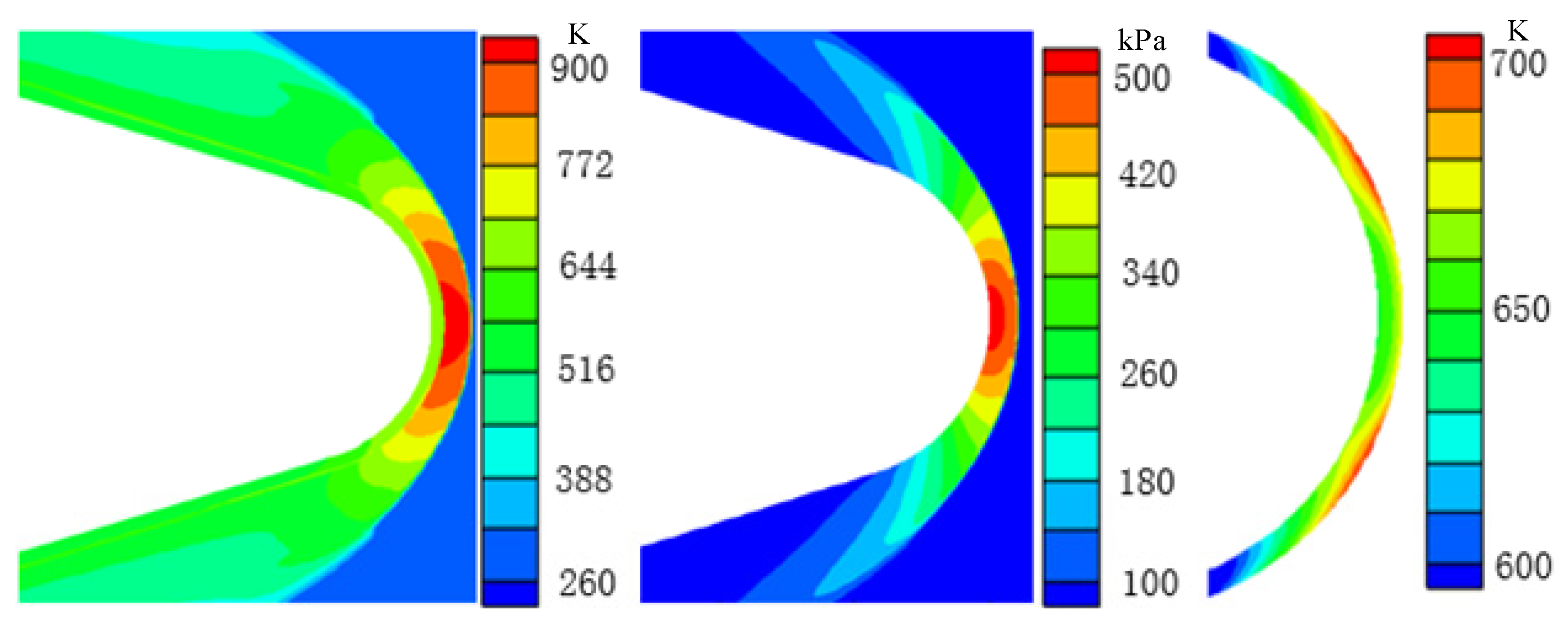
Figure 19 shows the results at 38 s when the flight altitude is around 9.5 km. This is the stage where the aircraft is accelerating but has not yet entered the hypersonic flight state. The maximum temperature of the external flow field increases to over 900 K, and the temperature of the external flow field near the optical dome is higher than that of the other positions of the aircraft structure. At this time, due to the improvement in the pneumatic heating intensity and sufficient heat conduction time inside the structure, the optical dome temperature is close to 650 K. With the increase of the flight velocity, the shock wave becomes increasingly intense. The wave angle decreases, and the parameter changes before and after the shock wave increase. From the pressure of the external flow field, it can be seen that the pressure near the back reaches 500 kPa, which is close to 5 atm. From the temperature distribution of the optical dome, it can be seen that the maximum temperature is over 700 K, and the temperature difference in the radial and circumferential structure inside the optical dome increases. This leads to changes in the heat flux distribution between the external flow field and the optical dome and the difference in the intensity of radiation heat dissipation in the sapphire optical dome.
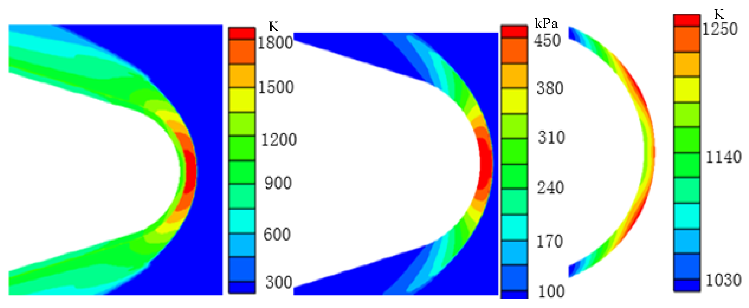
Figure 20 shows the results at 53 s when the flight altitude is around 17 km. After a period of acceleration, the flight velocity exceeds Mach 5, and the aircraft enters the hypersonic flight state. The maximum temperature of the external flow field exceeds 1800 K, which shows the severity of aerodynamic heating of the optical dome during hypersonic flight. With the increase in the flight velocity, the temperature of the flow field behind the shock wave increases due to intense compression. The temperature of the hypersonic aircraft structure continues to increase due to the increasing external aerodynamic heating. From the temperature distribution of the optical dome, it can be seen that the maximum temperature near the outer wall is 1250 K, and the minimum temperature on the inner wall is over 1030 K.
From the pressure distribution of the external flow field, it can be seen that the maximum pressure on the optical dome is approximately 450 kPa and remains at a high level during the whole flight. From the maximum pressure shown in
Figure 17 and the analysis of the results at 38 s, it can be observed that the high-pressure interval between 38 s and 53 s is mainly due to the strong pressure increase after the shock wave caused by the continuous acceleration of the aircraft, and the increase in the flight altitude leads to a decrease in the inflow pressure.
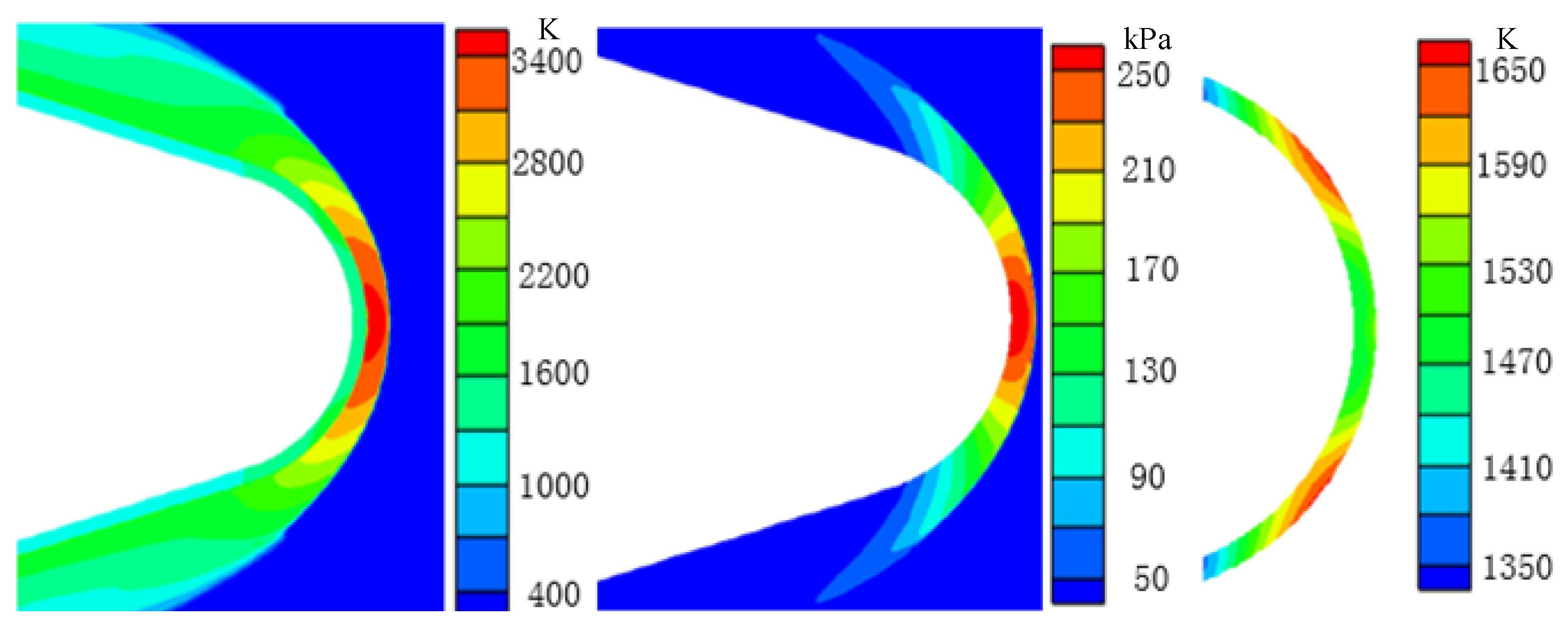
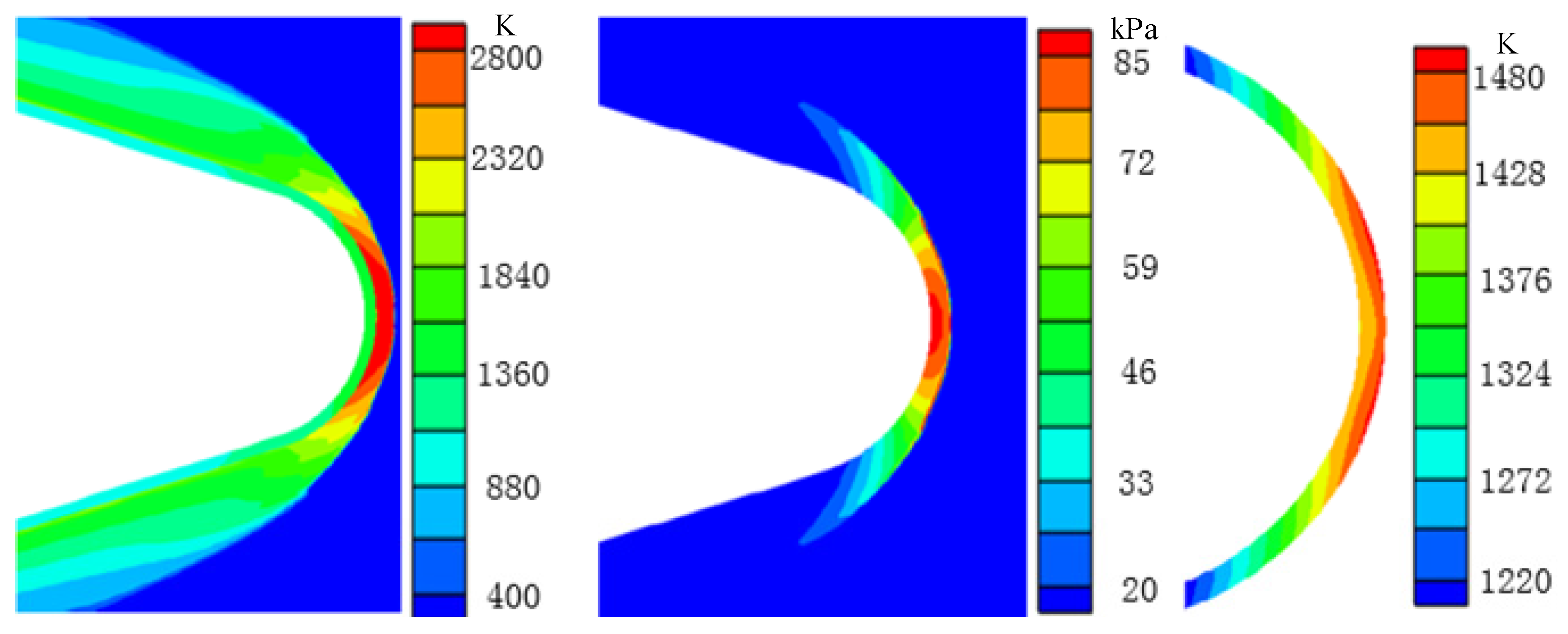
Figure 21 shows the results at 70 s; the first high-temperature cusp appears at this moment. At this moment, the flight altitude is around 24 km, the flight velocity is 2528 m/s, and the maximum temperature of the external flow field near the optical dome is over 3400 K. The aerodynamic heating effect is the strongest, the structure temperature reaches the peak, and also the radiation heat dissipation reaches the highest value. The moment when the temperature reaches its maximum is not the moment when the velocity reaches its maximum because of the dynamic balance between aerodynamic heating and radiation heat dissipation. In addition, the internal heat conduction of the structure has a greater effect relative to aerodynamic heat and radiation heat transfer. Under the combined action of hypersonic aerodynamic heating, radiation heat dissipation, and heat conduction inside the structure, the temperature distribution of the optical dome structure is as shown in
Figure 21, from which it can be seen that the maximum temperature of the optical dome reaches 1650 K.
The inflow pressure is only 2320 Pa due to the flight altitude, which is less than one-fifth of the pressure at 53 s. The inflow velocity does not increase much. According to
Figure 21, the maximum pressure on the outer wall is approximately 250 kPa.
5.2. Analysis of Results in the Second Period
Figure 22,
Figure 23 and
Figure 24 show the results of the temperature field, pressure of the external flow field, and temperature distribution of the optical dome structure at different time points in the second period (between 70 s and 190 s), respectively.
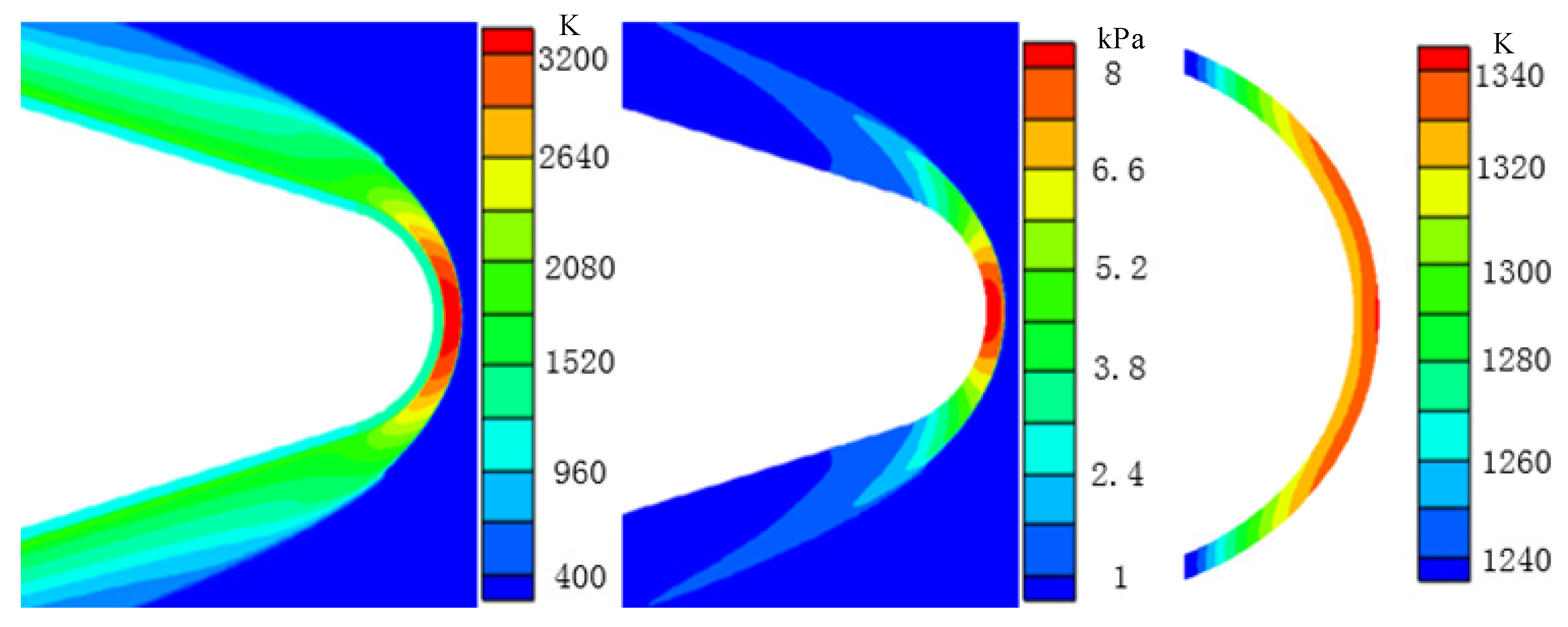
Figure 22 shows the results at 109 s, when the flight altitude is around 49 km; the velocity of the aircraft changes little during the second period. The velocity fluctuates at 2500 m/s from 70 s to 109 s. The maximum temperature of the external flow field is around 3200 K, which is slightly lower than that at 70 s, mainly because of the influence of flight altitude on the inflow parameters. The decrease in the inflow temperature not only directly affects the temperature behind the shock wave but also affects the local sound speed. As the Mach number is the ratio of the inflow speed to the local sound speed, it affects the inflow Mach number and indirectly affects the temperature distribution outside the optical dome. Because of the weakening of external aerodynamic heating, the radiation heat dissipation becomes greater than the aerodynamic heating, and the temperature of the optical dome structure drops although the temperature of the external flow field is still high. The maximum temperature of the optical dome structure decreases from 1650 K to 1340 K at 70 s, and the temperature of the outer side wall decreases faster than that of the inner side wall.
From the pressure distribution of the external flow field, it can be seen that the maximum pressure on the optical dome at this time is only approximately 8 kPa and is at a relatively low level during the whole flight. As can be seen from the variation in the flight altitude with time shown in
Figure 13, the flight altitude at this moment is close to the maximum flight altitude, the atmosphere is thin, and the inflow pressure is extremely low. The pressure on the optical dome wall shows a very low level.
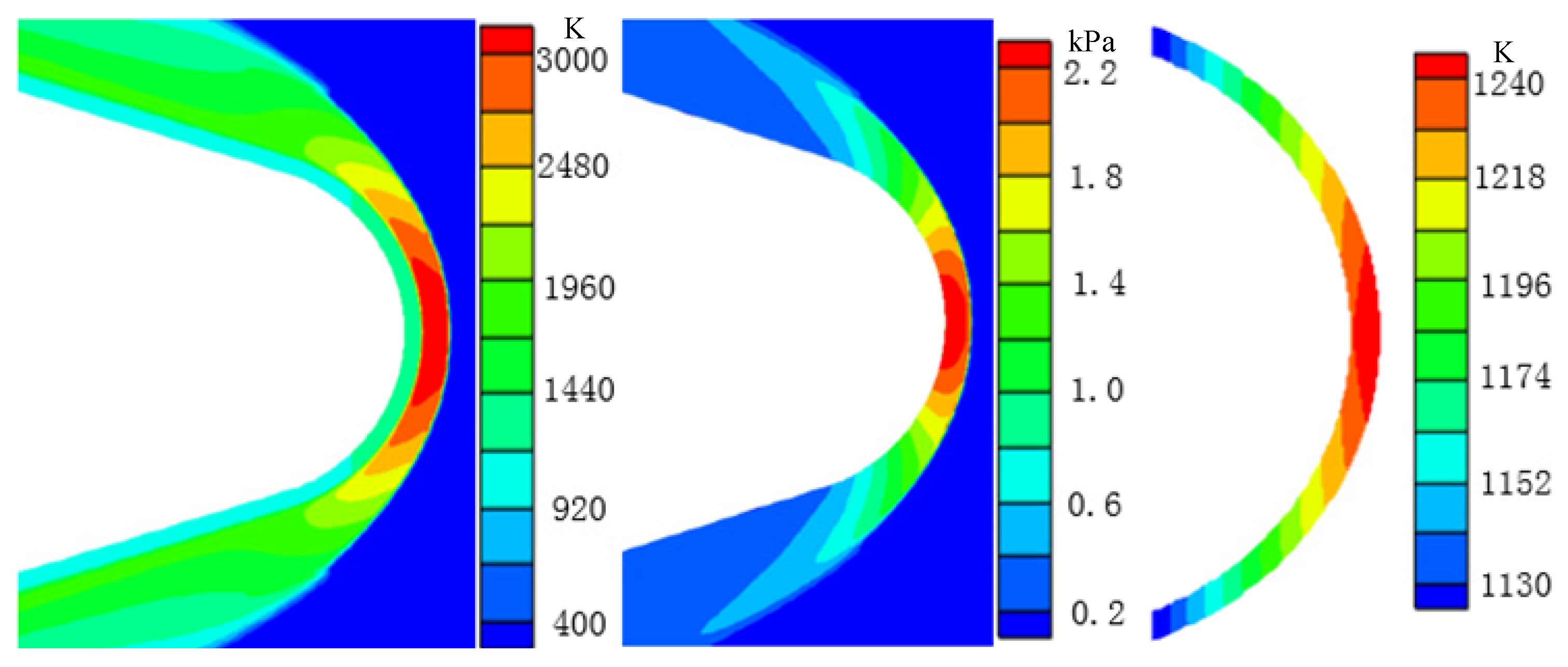
Figure 23 shows the results at 149 s, when the flight altitude is around 59 km, which is close to the maximum altitude of 60 km. The maximum temperature of the external flow field at this moment is approximately 3000 K, while the maximum wall pressure is only 2.2 kPa. The maximum temperature of the optical dome structure is approximately 1240 K. Compared with the results at 109 s, temperature of the external flow field, pressure of the external flow field, and internal temperature of the optical dome structure decrease. The reason for the decrease is similar to the analysis at 109 s. Due to the further increase of the flight altitude, the aircraft is in an atmospheric environment with low temperature, low pressure, and low density (thin air). The aerodynamic heating effect continues to weaken, while the radiation heat dissipation continues to strengthen due to the fourth square correlation with the structure temperature, resulting in the decrease of the optical dome structure temperature. The pressure on the optical dome wall remains extremely low due to the low-pressure environment.
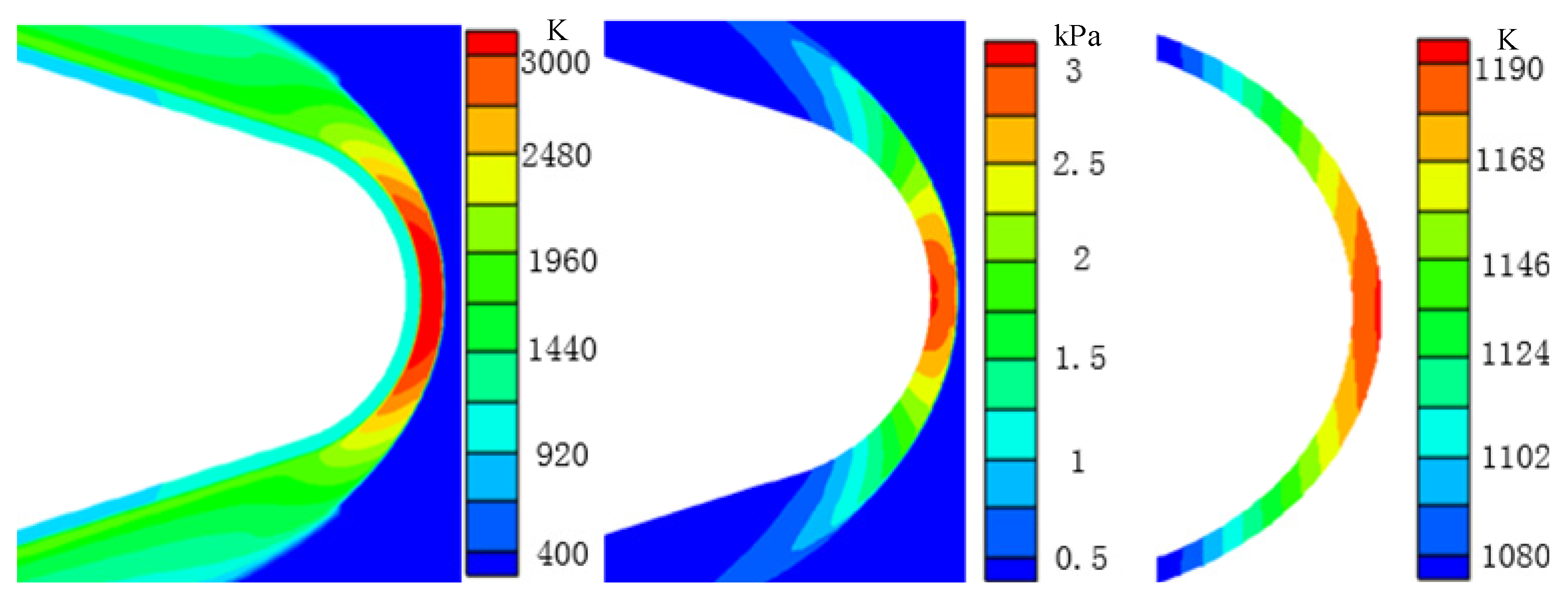
Figure 24 shows the results at 190 s, which is the low-temperature cusp of the optical dome structure temperature in the flight. The flight altitude is around 55 km, and the aircraft has just entered the reentry phase. At this moment, the maximum temperature of the external flow field near the optical dome remains at approximately 3000 K, but the structure temperature continues to decrease, and the maximum temperature of the optical dome structure is less than 1200 K. The cooling effect in this stage is mainly accomplished by the radiation of the optical dome structure, and the rate of change of aerodynamic heating in the external flow field is very small. As the structure temperature continues to decrease during this period, it adversely affects the radiation and heat dissipation, gradually weakening it and reaching a new balance with the aerodynamic heating. The wall pressure at this moment is still at a low level due to the flight altitude, and the maximum wall pressure is only 3 kPa.
5.3. Analysis of Results in the Third Period
Figure 25 and
Figure 26 show the results of the temperature field, the pressure of the external flow field, and the temperature of the optical dome structure at 239 s and 290 s, respectively. At 239 s, the flight altitude decreases to around 33 km, and the flight velocity decreases slightly compared with the second period. The temperature of the external flow field near the optical dome is above 2800 K, and the maximum temperature is around 3000 K. As the optical dome has cooled to below 1200 K in the second period, the average temperature difference between the optical dome structure and the external flow field near the optical dome increases to nearly 2000 K. This temperature difference increases the intensity of aerodynamic heating and the balance between aerodynamic heating and radiation heat dissipation no longer exists. The temperature outside the optical dome increases, and the heat is transferred inside. The maximum temperature of the optical dome structure increases to over 1480 K at this moment, and the temperature of the optical dome edge and inner wall surface increases to over 1220 K. It can be seen from the pressure of the external flow field that the pressure near the back cover wall of the shock wave increases to 85 kPa. This is mainly due to the decrease in flight altitude and denser air than that at 190 s; thus, the inflow pressure increases, which is finally reflected in the increase in the pressure on the optical dome wall.
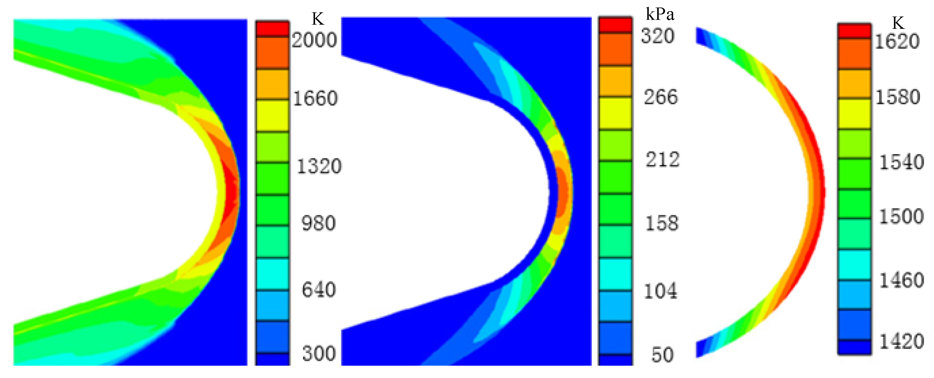
Figure 26 shows the results at 290 s, when the flight altitude decreases to around 20 km, and the optical dome structure temperature increases to the second temperature peak after this time period. With the decrease in flight velocity, the maximum temperature of the external flow field decreases to approximately 2000 K. Before this moment, the dominant aerodynamic heating effect continues to decrease, while the previously weak radiation intensity continues to increase due to the continuous increase in the temperature of the optical dome structure. This phenomenon continues until 290 s, when there is a new thermal equilibrium state, exhibiting the second temperature peak. At this time, the maximum temperature of the optical dome structure is 1620 K, and the minimum temperature inside is around 1420 K.
The pressure of the external flow field is affected by the decrease in the flight altitude, and the pressure of the atmospheric inflow increases during this period, leading to the continuous increase in the pressure of the external flow field. At 290 s, the maximum pressure on the optical dome wall is 320 kPa.
5.4. Analysis of Results in the Fourth Period
Figure 27 and
Figure 28 show the results of the temperature field, pressure of the external flow field, and temperature distribution of the optical dome structure at 310 s and 330 s, respectively.
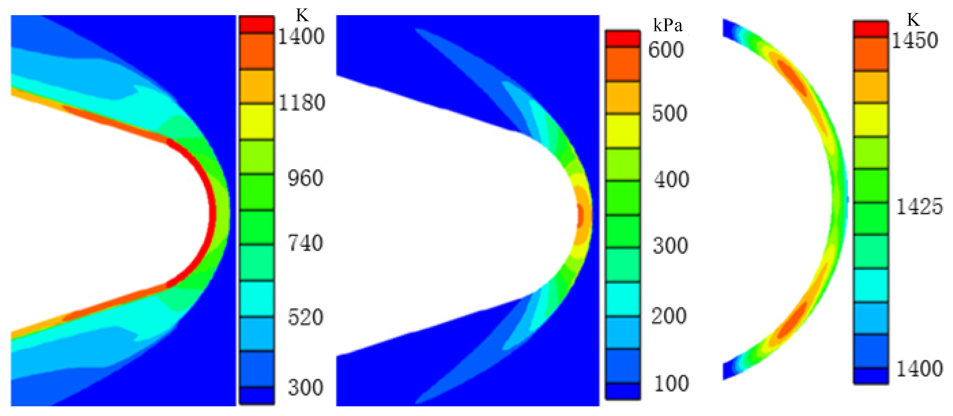
At 310 s, the flight altitude decreases to approximately 9.3 km, and the flight velocity decreases to 1178 m/s. During this period, the aircraft slows down to prepare for landing. The temperature of the aircraft structure at this moment is already higher than the temperature behind the shock wave of the external flow field, that is, the optical dome began to convectively dissipate heat to the flow field. The radiation effect of the optical dome is still evident. Under the dual effects of convection and radiation, the optical dome structure temperature begins to decrease.
As the flight altitude decreases, the inflow pressure increases rapidly. Because the flight velocity is still 1178 m/s, the pressure rise after the shock wave is still evident. Under the influence of Mach number and inflow pressure parameters, the stagnation pressure of the optical dome is greater than 600 kPa.
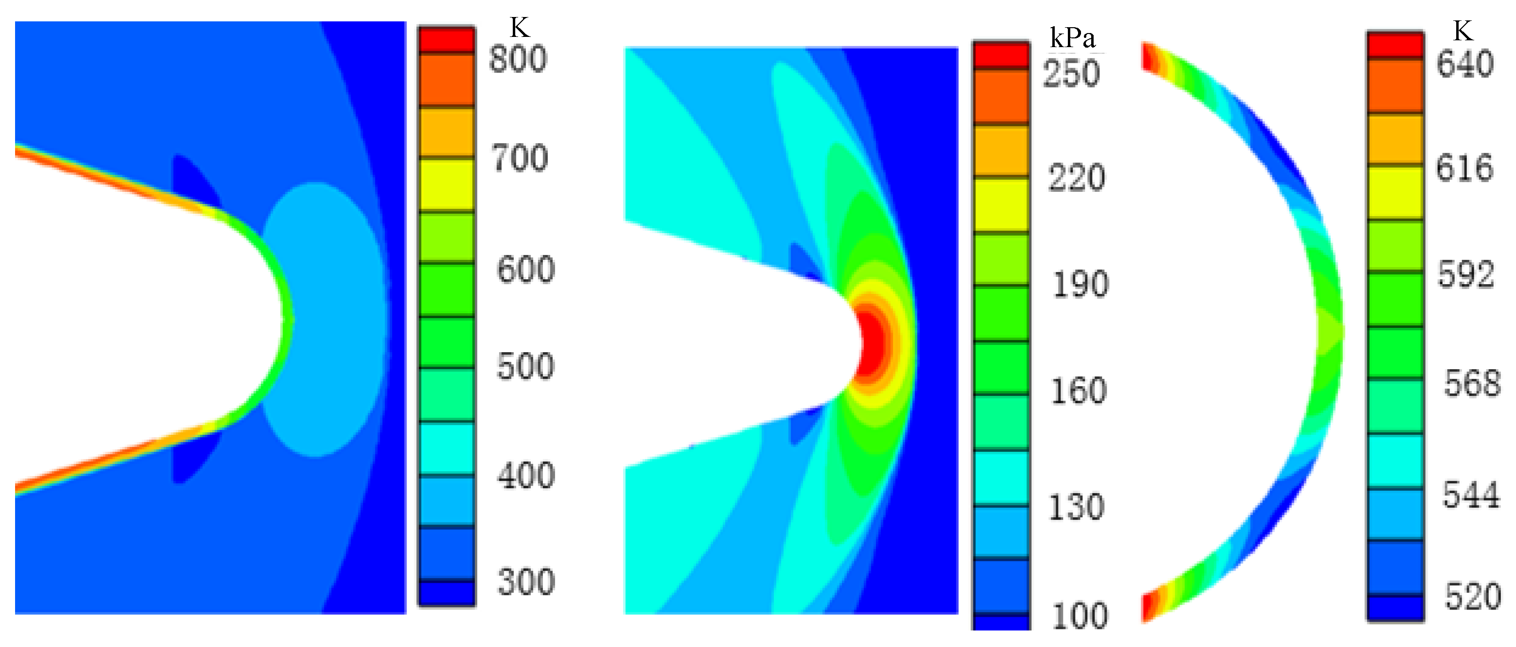
Figure 28 shows the results of the final moment of the whole flight when the flight altitude is close to the ground. At this moment, due to the continuous decrease in flight velocity, the shock angle of the detached shock wave on the nose of the aircraft is very large, and the parameters before and after the shock wave change only slightly. The temperature of the optical dome structure is higher than the maximum temperature of the flow field, and heat is continuously dissipated through convection and radiation. The maximum temperature of the optical dome structure is approximately 640 K. The temperature of the conical section behind the optical dome is higher than that of the optical dome. Due to the internal heat conduction of the aircraft structure, the temperature gradient between the titanium-alloy conical section and the sapphire optical dome leads to heat transfer from the conical section to the optical dome; thus, the temperature at the position where the titanium-alloy conical section is connected to the optical dome is higher than that at other positions of the optical dome.
Because of the rapid decrease in flight velocity, the effect of the pressure of the aircraft after the shock wave is greater than that caused by the altitude change of the aircraft. The atmospheric pressure parameters at the altitude of 9.3 km at 310 s show little difference with those at the altitude near the ground. It can be seen from
Figure 14 that the flight velocity at 330 s roughly decreases by half compared with that at 310 s. Therefore, the maximum wall pressure during this period decreases continuously, and the maximum wall pressure at 330 s is only 250 kPa.
6. Conclusions
In this study, the aerodynamic heat transfer characteristics of a hypersonic aircraft optical dome are studied, and the main conclusions are listed as follows:
(1) The distribution of average and maximum temperature on the inner and outer walls of the optical dome exhibit an M-shaped pattern, with two high-temperature cusps (70 s and 290 s) and one low-temperature cusp (190 s), and the highest average temperature coincides with the maximum wall temperature. Heat conduction in the optical dome and radiation in the high-temperature areas balance the wall temperature distribution.
(2) The wall pressure of the hypersonic aircraft changes with time during the whole flight process, showing the characteristics of high pressure at both ends of the time period and low pressure in the middle. The initial increase in the optical dome pressure is due to the rapid increase in flight Mach number, and the subsequent decrease is due to the decrease in flight altitude, leading to the decrease of inflow pressure. The reentry pressure firstly increases and then decreases, but the pressure on the optical dome wall increases continuously due to the altitude decrease. The pressure on the optical dome wall decreases due to the sharp decrease in Mach number.
(3) From 20 s to 290 s, the temperature of the external flow field near the optical dome is higher than that near other positions of the aircraft structure. Because of the severe aerodynamic heating of the nose during hypersonic flight, with the increase in flight velocity, the gas behind the shock wave of the external flow field is compressed more violently, resulting in an increase in the temperature.
(4) The structure temperature of the hypersonic aircraft is higher than the temperature behind the shock wave in the external flow field at 310 s and later. At this time, the optical dome begins to dissipate heat convection to the flow field, and the radiation effect of the optical dome is still obvious. Under the dual effects of convection and radiation, the optical dome temperature begins to decrease.


