Article

Prediction of Building Electricity Consumption Based on Joinpoint−Multiple Linear Regression

1
School of Architecture, Huaqiao University, Xiamen 361021, China
2
Xiamen Key Laboratory of Ecological Building Construction, Xiamen 361021, China
3
Data-Centric Engineering, The Alan Turing Institute, The British Library, 96 Euston Road, London NW1 2DB, UK
*
Authors to whom correspondence should be addressed.
Energies 2022, 15(22), 8543; https://doi.org/10.3390/en15228543
Submission received: 11 October 2022 / Revised: 4 November 2022 / Accepted: 9 November 2022 / Published: 15 November 2022

Abstract

:
Reliable energy consumption forecasting is essential for building energy efficiency improvement. Regression models are simple and effective for data analysis, but their practical applications are limited by the low prediction accuracy under ever-changing building operation conditions. To address this challenge, a Joinpoint–Multiple Linear Regression (JP–MLR) model is proposed in this study, based on the investigation of the daily electricity usage data of 8 apartment complexes located within a university in Xiamen, China. The univariate model is first built using the Joinpoint Regression (JPR) method, and then the remaining residuals are evaluated using the Multiple Linear Regression (MLR) method. The model contains six explanatory variables, three of which are continuous (mean outdoor air temperature, mean relative humidity, and temperature amplitude) and three of which are categorical (gender, holiday index, and sunny day index). The performance of the JP–MLR model is compared to that of the other four data-driven algorithm models: JPR, MLR, Back Propagation (BP) neural network, and Random Forest (RF). The JP–MLR model, which has an R2 value of 95.77%, has superior prediction performance when compared to the traditional regression-based JPR model and MLR model. It also performs better than the machine learning-based BP model and is identical to that of the RF model. This demonstrates that the JP–MLR model has satisfactory prediction performance and offers building operators an effective prediction tool. The proposed research method also provides also serves as a reference for electricity consumption analysis in other types of buildings.

1. Introduction

Energy consumption analysis and forecasting in buildings are prerequisites for building energy efficiency improvement. In the design planning stage, the design of building energy use systems can be improved. In the operation stage, reasonable energy consumption forecasting can help operators identify energy-saving potential and implement scientific management policies. Usually, the model for building energy consumption prediction is composed of three components [1]: input data (e.g., architectural design parameters such as orientation [2], shape [3], the window-to-wall ratio [4], shading [5], and weather variables), system structure (e.g., thermal properties of the exterior walls [6,7], parameters of the cooling or heating system [8,9]), and output data (i.e., energy use).
Currently, there are numerous methods for predicting building energy consumption, which can be grouped into 2 categories depending on the analysis method [10]: simulation techniques based on physics principles and data-driven approaches utilizing artificial intelligence algorithms.
Simulation techniques are used to predict building energy consumption by building physical models. Currently, there are several software tools for building energy consumption simulation, such as DOE-2 [11], Energy Plus [12], ESP-r [13], TRNSYS [14], Design Builder [15] and EQUEST [16], etc. These tools can calculate the changes in building energy consumption on a time-by-time basis and are easy and convenient to operate.
The data-driven approach applies statistical analysis approaches to build mathematical models of energy consumption systems based on known input and output data. Data-driven models used in the field of energy prediction involve Multiple Linear Regression (MLR) [17], Time Series Model (TSM) [18] and machine learning-based methods, e.g., Back Propagation (BP) neural network [19] and Random Forest (RF) [20].
The Joinpoint−Multiple Linear Regression (JP–MLR) model proposed in this study is a regression model based on a data-driven approach. Each algorithm has its advantages and disadvantages, and choosing the right method for a specific case is the key to ensuring the success of building energy operation management. However, different models in the data-driven method have different prediction accuracy. Sretenović [21] used different inverse modelling methods, including MLR, SVM and neural network models, to compare the prediction of cooling electricity consumption in a commercial building in Belgrade. The results show that the MLR model has the lowest accuracy than the neural network and SVM.
The following authors have also used regression models for energy forecasting. Fumo et al. [22] analyzed the energy consumption of residential buildings using MLR and quadratic regression. Two explanatory variables were used in the model: solar radiation and outdoor temperature. However, they found that the root mean square error values deteriorate with the inclusion of the solar radiation variable in the model. The prediction accuracy of the model for daily data R2 = 74%. Amiri et al. [23] demonstrated the advantages and potential of the MLR regression model for building energy prediction through 150,000 computer simulations. The model contains 13 screened building parameters, of which occupancy schedule and exterior wall construction are the two most dominant parameters. The R2 values of the models given in the study vary between 95% and 98%, but there are no other parameters for model evaluation that can be discussed. Marwen et al. [24] used an MLR regression model to predict the future electricity consumption in Florida. The results show that month, cooling and heating degree days and GDP are the important variables in the regression model. Venkataramana et al. [25] found that the MLR method can predict the electricity demand of a substation located in Warangal with good accuracy. YANG et al. [26] found a strong relationship between outdoor temperature and building energy usage utilizing a regression method and established a cubic equation with R2 = 70.27%. Capozzoli et al. [27] analyzed the annual heating energy consumption of 80 schools and developed an MLR model with 9 variables to estimate the energy consumption of these schools. The final model showed R2 = 85% and MAPE = 15%. Aranda [28] developed three different MLR models using building characteristics and climatic areas to assess the energy performance of bank buildings in Spain. The R2 values for the three models were 56.8%, 65.2% and 68.5%, respectively.
Based on the above discussion, we found four deficiencies in the existing regression prediction model studies.
First, previous regression analysis studies have been based on MLR analysis, and the Joinpoint Regression (JPR) method has not been addressed. The JPR model is a special regression model [29] that is typically employed in the field of medicine [30].
Second, the accuracy of regression models is relatively low compared to other data-driven models. To increase the accuracy of regression models, researchers have to find more input variables. As the input variables to the regression model are critical, the number and validity of the variables can significantly influence the predictive accuracy of the model. However, the variables affecting the model cannot always be obtained effectively. Moreover, some variables are difficult to measure in practical applications. Therefore, the issue of using the current regression modelling techniques logically and producing great predicted performance is still present given the small number of critical variables.
Again, previous research has shown a significant relationship between energy use and meteorological variables, and the models they constructed used meteorological variables like air temperature, but the impact of rain or shine is often overlooked. Rainy (or sunny) weather affects people’s travel plans and indirectly affects the use of indoor appliances, thus affecting energy consumption. Therefore, in this study, the input parameters of the model are studied by considering whether it rains or not on the same day.
Finally, previous studies have included the key meteorological variable, i.e., outdoor air temperature, in the input variables of the model. However, most of them ignored the effect of balance point temperatures on energy consumption. The balance point temperature is the turning point at which the correlation between a building’s energy consumption and outdoor temperature changes. For example, rising temperatures would raise the need for interior cooling and vice versa. The electricity usage changes at different rates above or below the temperature point. Thus, when predicting building energy consumption, it is important to take into account the influence of the balance point temperature and perform the analysis in segments.
In order to overcome the problems mentioned above, this study analyzes the daily electricity consumption data of 8 apartment buildings in Xiamen, China, and proposes a building energy consumption prediction model based on Joinpoint−Multiple Linear Regression (JP–MLR). To the best of the authors’ knowledge, this work is the first to apply the JPR model to the field of electricity prediction. A total of 8 variables are screened in the pre-analysis phase of the study, and 6 parameters are finally selected as model variables.
The rest of the paper is structured as follows. Section 2 introduces the methodology of this study. Section 3 is a case study that demonstrates the application of the proposed method. Section 4 presents a comparison and discussion of the model’s performance. Finally, Section 5 gives concluding remarks.

2. Methodology

This section presents the research methodology of the proposed JP–MLR model, the framework of which is shown in Figure 1. The details of the different stages are detailed in the following.

2.1. Data Collection

In this research, electricity consumption data from eight student apartment buildings located in Xiamen, China, are analyzed to apply and validate the proposed JP–MLR model, as shown in Figure 2. The electricity consumption data are measured through a central smart meter on the campus. In addition to this, meteorological data and gender information of occupants are also collected. The meteorological data are downloaded from a meteorological website [31].
This study spans a full academic year (the academic system of Chinese universities, which includes two semesters). The first semester is from 1 September 2020 to 8 January 2021, and the second semester is from 15 March 2021 to 2 July 2021, for a total of 240 days.
The dependent variable in the prediction model is the electricity consumption of the building. There are three types of indicators that describe the electricity consumption of a building: total electricity consumption, electricity consumption per floor area, and electricity consumption per person [32]. Since the floor area and occupancy of the apartments are the same, the average daily electricity consumption of the rooms is chosen as the dependent variable data in this study.
A total of 8 explanatory variables were collected and divided into continuous and categorical types. The continuous variables are mainly outdoor meteorological parameters, and there are 5 of them: average outdoor air temperature, average relative humidity, daily global irradiance, average wind speed and daily temperature amplitude, see Figure 3. There are 3 categorical variables: gender of the occupants, the holiday index and the sunny day index. These indices will be explained below.
Among these 8 apartment buildings, the odd-numbered buildings (1#A, 1#B, 3#A, 3#B) are male buildings and the even-numbered buildings(2#A, 2#B, 4#A, 4#B) are female buildings. Different genders have different energy consumption habits and electricity demands [33,34], thus using gender as one of the explanatory variables. The dummy value for the female is 0 and for the male is 1.
Building occupancy significantly affects the energy consumption of a building. However, the real building occupancy rate is not available in the actual study, so this research introduces the “holiday index” to represent the building usage [17]. The dummy value for working days is 0 and for holidays is 1. Non-working days include weekends and national holidays [35]. The holiday index affects the occupancy of the building and thus the use of indoor electrical equipment.
The sunny day index is a meteorological parameter of categorical type. Rain or shine affects people’s travel arrangements, and therefore indirectly reflects the use of electrical appliances inside the building. Therefore, this study introduces a proxy variable, the “sunny day index”. The dummy value is 1 for rainy days and 0 for non-rainy days. This is one of the innovative points of this study.
Since the parameters such as floor area, orientation and indoor electrical equipment (including air conditioning) are the same for these 8 buildings, these parameters are not considered explanatory variables in this study. In this study, the data from Building 2#–4# are used as the training data set and Building 1# is used as the testing data set.

2.2. Data Preprocessing

The existence of missing-value rooms, empty rooms and data-abnormal rooms can interfere with the statistical calculation of average electricity consumption, so data pre-processing is required to identify and remove them from the data set, as shown in Figure 4. When the electricity usage in a room has not been recorded for more than 3 days, it is recognized as a missing-value room, which may be caused by a faulty electricity meter. However, to save sample size, rooms with only one or two missing values are filled by linear interpolation. When zero or near-zero electricity use in a room is last for more than five consecutive days, this room is deemed to be empty. When negative electricity use is observed in a room, this room is considered to be data-abnormal. After data pre-processing, 493 valid rooms remained in the dataset.

2.3. Data normalization

Data normalization is an important part of regression analysis. Different input variables have different magnitudes, which can lead to weak comparability between variables. In order to enhance the analysis results of the data, data normalization is required. After the raw data are normalized, the variables are in the same order of magnitude and dimensionless, which is suitable for data analysis. There are various methods of data normalization [36], such as Min-Max Normalization, Z-score Normalization and Batch Standardization. The Z-score normalization method was chosen for this study:
x n =   x u δ
where xn is the normalized data, x is the original data, u is the mean of the original data and δ is the standard deviation of the original data. The processed data have a mean of 0 and a variance of 1, which conform to the standard normal distribution and are dimensionless.

2.4. Model Analysis Method

2.4.1. Joinpoint Regression (JPR)

The JPR method is first proposed by KIM in 1998 [29]. It performs a regression analysis on each side of a join point of trend change after identifying it. JPR is typically employed in the field of medicine [37] for the analysis of time series, such as the trend in the incidence of a disease over a decade. However, the JPR method can also be utilised for datasets where the independent parameter is ordered numerical and the dependent parameter is numerical. This method was also used in this study to analyze balance point temperatures. The Joinpoint Regression Program (version 4.8.0.0) was released by the National Cancer Institute [38].
For a set of ordered data (xi, yi),…,(xn, yn), where yi is the dependent variable, xi is the independent variable, and x1 ≤…≤ xn. The log-linear model equation is:
E [ y i | x i ] = e β 0 + β 1 x i + δ 1 x i τ 1 + + + δ k x i τ k +
where β0 is the constant, β1 is the regression coefficient; δ k = β n + 1 β n is the coefficient of the segments; τk is the joining point, k is the number of joining points, when ( x i τ k ) > 0 , x i τ k + = ( x i τ k ) otherwise, ( x i τ k ) = 0.

2.4.2. Multiple Linear Regression

MLR is a statistical tool [39] used to reveal the linear relationship between the dependent variable and multiple other explanatory variables.
The MLR equation is:
Y = b 0 + b 1 x 1 + b 2 x 2 + + b n x n
where Y is the predicted value, x1 to xn are the different explanatory variables, b0 is the intercept, and b1 to bn are the regression coefficients.
The check for collinearity between explanatory variables is crucial in the analysis of MLR models. The presence of high collinearity between explanatory variables can affect the calculation of the regression model. When multiple explanatory variables are co-linear, one should choose to keep and remove the others. The analysis of MLR is performed using SPSS25 software [40].

2.4.3. Back Propagation Neural Network

Back Propagation (BP) neural network is a weight learning process based on error back propagation of gradient most rapid descent method [41]. Its network learning process is the process of iterating weights and thresholds to make the error reach a preset range. The BP algorithm includes two phases: the forward spread of the signal and the backward spread of the error. The errors are evaluated in the direction from input to output, while adjusting the weights and thresholds in the opposite direction. This part of the computation is programmed in Python, using the scikit-learn library (https://scikit-learn.org/, accessed on 4 November 2022). The training process is as follows.
  • Sample data selection and grid initialization, initialization of BP neural network weights and thresholds.
  • Preprocess the sample data and calculate the hidden layer and output layer outputs. Suppose there are s neurons in the hidden layer, the output of the hidden layer is bj, and the threshold of the hidden layer and output layer units are θj θk, respectively. Then, the output of the jth unit of the hidden layer, bj, is:
    b j = f 1 j = 1 s w ij x i θ j
  • The output layer outputs yk as:
    y k = f 2 j = 1 s w ij b j θ k
    where f1, f2 are the hidden layer and output layer transfer functions, respectively.
  • Deviation function of the actual output value of the neural network from the expected value.
    e = k = 1 m ( t k y k ) 2
  • If the prediction error does not meet the setting requirements, the error is back-propagated and the weights and thresholds of the network are adjusted iteratively. The above process is repeated until the error meets the pre-set requirements.
Figure 5 shows the computational structure of the BP neural network.

2.4.4. Random Forest Model

Random forest (RF) is a combinatorial model containing multiple decision trees [42], which has the advantages of high accuracy, flexibility, ability to handle high-dimensional feature samples, and the ability to evaluate the importance of individual features. RF is an improved algorithm for integrated learning [43], and its principle is shown in Figure 6. The RF algorithm randomly samples m training sets with the same sample size as the original sample and builds m decision trees from the original sample. The final result of the RF regression, y(x), is determined by the average of the outputs of the m decision trees.
y x = 1 m h x , θ n
where x is the independent and dependent variables of the input model. θn is the independent identically distributed random vector. This part of the computation is also programmed in Python, using the scikit-learn library.

2.5. Model Performance Evaluation

To quantitatively evaluate and compare the forecasting performance of different data-driven algorithms, this study evaluates the results using 6 metrics commonly used in electricity load forecasting [17,44]: the Root Mean Squared Error (RMSE), the Coefficient of Variation of the Root Mean Squared Error (CV-RMSE), the Normalized Mean Bias Error (NMBE), the Normalized Root Mean Square Error (NRMSE), the Mean Absolute Percentage Error (MAPE) and R2. The above metrics are calculated in Equations (8)–(13), where yi is the real value, y ^ i is forecasted value and y - is the mean of the real values. Index “n” represents the total number of observations.
RMSE = i = 1 n y i y ^ i 2 n
CV-RMSE =   RMSE y ¯   ×   100 %
NMBE =   i = 1 n ( y i ŷ i ) n × y ¯ × 100 %
NMBE =   RMSE y max y min
MAPE =   1 n i = 1 n ŷ i y i y i × 100 %
R 2 = 1   i = 1 n y i y ^ i 2 i = 1 n y i y ^ i 2

3. Results and Analysis

Air temperature is the most important factor affecting energy consumption [45,46]. A good prediction can be achieved by establishing a one-dimensional equation using outdoor air temperature as the independent variable, R2 = 0.7027 [26]. Therefore, as shown in the review in Section Introduction, most of the MLR models developed by previous authors include air temperature among the explanatory variables. However, the simple MLR prediction model has a large error and does not consider the effect of balance point temperatures on energy consumption.
Xiamen is located in China’s hot summer and warm winter climate zone, with cooling in summer and almost no heating in winter. In addition, campus administrators procured air conditioners in the rooms without heating functions to save energy. This results in a significant correlation between electricity use and the outdoor air temperature during the hot season, and no significant correlation during the cold season. The trend of electrical consumption should be different at different temperature conditions. Therefore, a segmented regression approach should be used for the temperature parameter-driven electric consumption prediction model according to the balance point temperatures.
The JPR analysis is carried out with average energy usage as the dependent parameter and temperature as the independent parameter, the results are shown in Figure 7. Additionally, Table 1 shows their parameters. Model B is chosen because it fits better and has more significant parameters than Model A. It can be expressed as
f ( T ) = exp { 0.399864 + 0.012426 T + 0.296417 ( T 20.5 ) + 0.2056766 T 26.0 + }
where f(T) is the predicted mean daily electricity usage, T is mean daily temperature. The range of T is 6.31−31.45 °C.
From Model B, it can be observed that two balance point temperatures exist that influence the energy usage curve of the buildings, 20.5 °C and 26.0 °C, respectively. The average outdoor air temperature can be divided into three segments based on these two turning points. The Segment Ⅰ is the low-temperature segment, where the average outdoor air temperature value is lower than 20.5 °C. Segment Ⅱ is the transition segment, where the temperature is between 20.5 and 26.0 °C. Segment Ⅲ belongs to the high-temperature segment, the temperature is greater than 26.0 °C. At lower temperatures (<20.5 °C), the room does not need to be cooled and only basic energy consumption such as lighting or sockets is included, so energy consumption is independent of temperature. The energy consumption remains almost at a stable value because the users have the same daily habits. At high temperatures (>26.0 °C), the energy use is significantly correlated with temperature because the daily energy consumption is mainly cooling energy consumption. Additionally, in the transition temperature segment (20.5–26.0 °C), such as spring or fall, the temperature change significantly affects the occupants’ hot and cold sensations. It is the key stage to decide whether to turn on the air conditioner or not, so there is a clear rising curve here.
The R2 value of model B is 94.34%, which is already much better than the simple MLR model (R2 = 72% in [17]), while 5.66% of the variables (ΔEd) are still influenced by unknown or potential factors. So the perfect prediction model can be expressed as Equation (15).
Ed = f(T) + ΔEd
Therefore, to further refine the model, ΔEd is analyzed using the MLR method, where ΔEd is the difference between Ed and f(T). Ed is the predicted daily electricity consumption. The ΔEd of three Segments are analyzed using the MLR method, respectively, and continuous-type independent variables are used with normalized data.
Firstly, the significance between the 8 explanatory variables and the dependent variable (ΔEd) is identified in Table 2. After preliminary tests, explanatory variables that are not significantly linearly related to the dependent variable are excluded (p-value > 0.05). In Segment Ⅰ, global solar irradiance, average outdoor air temperature, relative humidity, and wind speed are excluded. In Segment Ⅱ, all explanatory variables are significantly correlated with the dependent variable, so no explanatory variables are excluded. In Segment Ⅲ, the sunny day index and global solar irradiance are excluded.
Then, the explanatory variables suitable for inclusion in the model are selected based on the collinearity analysis, as shown in Table 3. Collinearity is a phenomenon in which independent variables (explanatory variables) are correlated with each other. High collinearity between any two variables indicates that only one of them can be used because they affect the dependent variable in a similar way. In Segment I of the model, 2 explanatory variables are chosen: gender (X2) and sunny day index(X3). In the Segment II, 3 explanatory variables are selected: holiday index (X1), gender (X2) and sunny day index (X3). In the Segment III, 3 explanatory variables are selected: holiday index (X1), gender (X2) and relative humidity (X6).
MLR analysis is performed using the selected explanatory variables, and the pa-rameters of the models for the 3 segments are calculated as shown in Table 4. All three segments of the model use the gender variable and have a positive slope. This indicates that males use more electricity than females, both in winter and summer, which is in line with previous works [34]. The sunny day index is used in both Segment I and II with a positive slope. This indicates that at relatively low temperatures, rainy days re-duce the occupants’ outside activities and thus increase indoor electricity usage. In Segments Ⅱ and Ⅲ, when the temperature is relatively high, the day type (i.e., working or not-working day) will also affect the electricity consumption of the day. The positive slope of the holiday index indicates that on non-working days, occupants do not have to go out to work or class, which leads to an increase in indoor electricity consumption. In addition, in Segment Ⅲ, i.e., at high temperatures, the relative humidity also affects the electricity consumption. A positive slope indicates that the higher the humidity, the higher the electricity consumption of the air conditioner will be.
The ΔEd is evaluated by the MLR method. The final integrated prediction model, i.e., the JP–MLR model, can be expressed as: when T ≤ 20.5 °C:
Ed = exp (0.399864 + 0.012426T) − 0.279 + 0.688x2 + 0.388x3
when 20.5 °C < T ≤ 26.0:
Ed = exp (−5.6766845 + 0.308843T) − 1.553 + 0.269x1 + 1.730x2 + 2.133x3
when T > 26.0 °C:
Ed = exp (−0.3290929 + 0.1031664T) − 1.766 + 1.199x1 + 2.77x2 + 0.386x6
which implies that Ed = f (T, x1, x2, x3, x6, x8), where T is average outdoor air temperature, x1 is holiday index, x2 is gender, x3 is sunny day index, x6 is normalized daily average relative humidity, x8 is normalized daily temperature amplitude and Ed is the predicted daily electricity consumption,.

4. Discussion and Comparison of Data-Driven Models Performance

Using data from the training set, five different data-driven algorithm methods are employed to predict the average daily electricity consumption in Building 1# (the test set). These five methods are: the JP–MLR model, JPR model, MLR model, BP model and RF model. Among them, JP–MLR, JPR and MLR are models based on regression algorithms, and BP and RF are models based on machine learning algorithms.
The analysis process and results of the JP–MLR model are shown in Section 3.
The JPR model derived using the training set data is f(T).
The algorithm of the MLR model is the same as when analyzing ΔEd in Section 3. The analysis process is divided into three steps: preliminary analysis, collinearity analysis and regression analysis. Preliminary and collinearity analyses are shown in Table 5. The p-value of the holiday index is greater than 0.05, so it can be excluded and thus collinearity is analyzed for the remaining seven variables. Gender (x2) has no collinearity with any of the other variables. In contrast, the collinearity between the six climate-related variables is more severe, so only one variable could be selected, and the average outdoor air temperature (x5) is chosen for this study.
MLR analysis is performed based on the two selected variables (x2, x5) and the results are shown in Table 6. The final model is shown in Equation (5), where x2 is the gender and x5 is the normalized average outdoor temperature.
Ed = 5.341 + 1.409x2 + 3.912x5
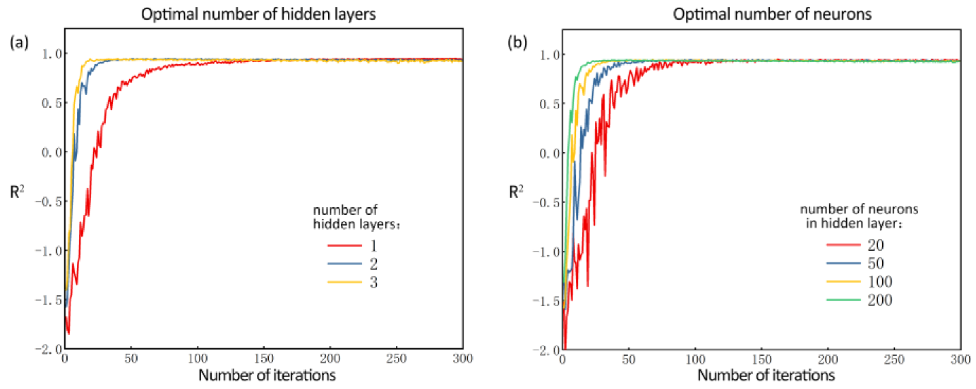
The BP model uses the 8 explanatory variables mentioned in this study as input variables, and the output variable is the average daily electricity consumption. The number of hidden layers, the number of neurons in the hidden layers, and the number of iterations are three hyperparameters that influence how well the BP model performs. Since there is no universal unique value for these hyper parameters, this study uses trial-and-error method for parameter tuning.
Firstly, the number of hidden layers is debugged. When the number of hidden layers is 1, 2 and 3, respectively, the R2 value of the BP model varies with the number of iterations, as shown in Figure 8a. The other parameters in the iterative process are set as follows: the number of neurons in the hidden layer is 100, and the number of iterations is 300. As the number of iterations increases, R2 increases continuously and the prediction accuracy improves, and the increase in the number of hidden layers speeds up the convergence of R2 to some extent. However, the effect of the number of hidden layers on the model accuracy tends to stabilize after a threshold (i.e., 40 for 1 hidden layer, 50 for 2 hidden layers and 150 for 3 hidden layers). To save training time at computation, 2 hidden layers with moderate convergence speed are chosen, since an increase in the number of hidden layers would cause a significant increase in training time.
Then, the number of neurons in each hidden layer is debugged. The number of neurons in the hidden layer is set to 20, 50, 100 and 200, respectively, and the effect of the number of neurons in the hidden layer on the prediction accuracy is analyzed. The other parameters in the iterative process are set as follows: the number of hidden layers is 2 and the number of iterations is 300. The change of R2 is shown in Figure 8b. With the increase of the neurons, the convergence speed of R2 accelerates to different degrees. The convergence speed at the neuron number of 200 is much higher than that at 20. But again, after many iterations, the accuracy of the model (R2) tends to be stable, and the prediction errors are the same for different numbers of neurons. Therefore, the hyper parameters of the BP model used as a comparison in this study are set as follows: the number of hidden layers is 3, the number of neurons is 200, and the number of iterations is 300.
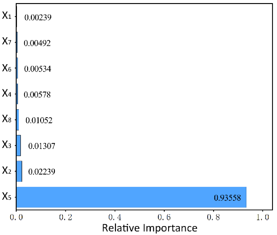
The RF model also uses the eight explanatory variables mentioned in this study as input variables and the output variable is the average daily electricity consumption. The main parameter that affects the performance of the RF model is the number of decision trees. The same, trial-and-error method is used to find the optimal number of trees. The model prediction accuracy is calculated sequentially for the number of trees from 1 to 300, still using R2 as the evaluation metric. As shown in Figure 9, the model is optimal when the number is 22, so this study uses this parameter setting to build the RF model. The importance of the eight input variables is shown in Figure 10, and the importance of temperature (x5) is much higher than the other variables. This also indicates that temperature is the most important factor affecting building energy consumption.
The final prediction results of the five models for Building #1 (test set) are shown in Figure 11, and their evaluation metrics are shown in Table 7. The predictive performance of the JP–MLR model far exceeded that of the conventional regression models (JPR and MLR), where all six evaluated metrics far outperformed them. The R2 values of the JP–MLR model were 8.11% and 24.79% higher than JPR and MLR, respectively. Compared to the machine learning models, the JP–MLR model outperforms the BP model and is basically on par with the RF model. The JP–MLR model outperformed BP in all six metrics, with CVRMSE and NMBE being 2.47% and 3.61% lower than BP, respectively. Even though the BP algorithm can be derived as neural networks for the task of regression, its prediction performance will be inferior to the JP–MLR model be-cause the influence of balance point temperature is not taken into account. CVRMSE and NMBE are the only metrics recommended by the American Society of Heating, Refrigerating and Air-Conditioning Engineers (ASHRAE) for the evaluation of energy forecasting models. Although the CVRMSE of JP–MLR is 1.13% higher than that of RF, the NMBE is 3.03% lower. Moreover, the R2 of JP–MLR and RF are nearly the same, with only a 0.19% difference, so the prediction performance of both models is the same. The reason is that the RF algorithm can be also regarded as a special type of segmented regression, which divides the data set into segments and analyzes them segment by segment. However, the JP–MLR model is simpler and does not require complex programming knowledge for building managers, so JP–MLR is more valuable for promotion.
In addition, according to the recommendation of ASHRAE [47], the prediction model of building monthly energy consumption should have an NMBE of 5%. However, the prediction granularity of the JP–MLR model is 24 h (one day), but its NMBE value reaches 4.05%, which is sufficient to show its excellent performance. The prediction accuracy of the same model for a day will be lower than that for a month.
Not surprisingly, the MLR model has the worst evaluation results, a result that is consistent with the findings of [21]. The JPR model, however, outperformed the MLR model, with an R2 16.68% higher. Because the JPR model is actually a combination of several MLR models, so it fits better than the MLR model. It is the JPR that has the advantage of segmental analysis and is therefore chosen to be used in this study to identify the balance point temperature that influence energy usage. Additionally, the R2 of the JP–MLR model is 7.67% higher than that of the JPR model, which is because the JP–MLR model evaluates the residual (ΔEd) on top of the JPR model and therefore improves the accuracy.
It is worth noticing that the subject of this study is in a hot summer-warm winter area, while the magnitude or number of balance point temperatures in other climatic zones may be different. However, the research method proposed can be used as a reference. Similarly, although the subject of this paper is apartment buildings, the research methodology and modelling process could be applied to other kinds of buildings, for example, residential or industrial buildings.

5. Conclusions

Efficient building energy forecasting is an important foundation for building energy efficiency management. This study proposes a method for predicting building energy consumption based on JP–MLR through the analysis of daily electricity consumption data from 8 apartment buildings in Xiamen, China. The method has been applied and validated in practical tests. The JPR approach is utilized to identify two balance point temperatures for these apartment buildings: 20.5 °C and 26.0 °C. Segmental modeling based on these temperatures and residuals is evaluated using the MLR method. Six explanatory variables are used in the model, including three continuous variables (average outdoor air temperature, average relative humidity and temperature amplitude) and three categorical variables (gender, holiday index, and sunny day index). JP–MLR model with RMSE = 1.183 kWh, CVRMSE = 16.26%, NMBE = 4.05%, NRMSE = 6.00%, MAPE = 12.70% and R2 = 95.77%. By comparing the six prediction evaluation metrics, the JP–MLR model has good prediction performance, much better than JPR and MLR based on conventional regression algorithms, and also better than BP based on machine learning, while basically on par with RF. This proves the feasibility of the JP–MLR model proposed in this study, and the research method also provides a reference for the analysis of electricity consumption in other types of buildings.

Author Contributions

Conceptualization, H.Y.; methodology, H.Y.; software, H.Y. and C.Z.; validation, M.R. and C.Z.; formal analysis, H.Y.; investigation, H.Y.; data curation, H.Y.; writing—original draft preparation, H.Y.; writing—review and editing, M.R. and C.Z.; visualization, H.Y.; supervision, M.R. and C.Z.; funding acquisition, M.R.; resources, C.Z. All authors have read and agreed to the published version of the manuscript.

Funding

This research was funded by National Natural Science Foundation of China, grant number 51678254.

Data Availability Statement

Not applicable.

Acknowledgments

Authors would like to offer special gratitude to Pengyuan Zeng at the Department of Informationization Development and Management, Huaqiao University for providing information and electricity data.

Conflicts of Interest

The authors declare no conflict of interest.

References

  1. ASHRAE. ASHRAE Handbook—Fundamentals; Inch-pound 2017 SI ed.; American Society of Heating, Refrigerating, and Air-Conditioning Engineers: Atlanta, GA, USA, 2013. [Google Scholar]
  2. Delgarm, N.; Sajadi, B.; Delgarm, S.; Kowsary, F. A novel approach for the simulation-based optimization of the buildings energy consumption using NSGA-II: Case study in Iran. Energy Build. 2016, 127, 552–560. [Google Scholar] [CrossRef]
  3. Yu, W.; Li, B.; Jia, H.; Zhang, M.; Wang, D. Application of multi-objective genetic algorithm to optimize energy efficiency and thermal comfort in building design. Energy Build. 2015, 88, 135–143. [Google Scholar] [CrossRef]
  4. Li, J.; Zheng, B.; Bedra, K.B.; Li, Z.; Chen, X. Evaluating the effect of window-to-wall ratios on cooling-energy demand on a typical summer day. Int. J. Environ. Res. Public Health 2021, 18, 8411. [Google Scholar] [CrossRef]
  5. Carlucci, S.; Cattarin, G.; Causone, F.; Pagliano, L. Multi-objective optimization of a nearly zero-energy building based on thermal and visual discomfort minimization using a non-dominated sorting genetic algorithm (NSGA-II). Energy Build. 2015, 104, 378–394. [Google Scholar] [CrossRef] [Green Version]
  6. Hamdy, M.; Nguyen, A.-T.; Hensen, J.L. A performance comparison of multi-objective optimization algorithms for solving nearly-zero-energy-building design problems. Energy Build. 2016, 121, 57–71. [Google Scholar] [CrossRef] [Green Version]
  7. Murray, S.N.; Walsh, B.P.; Kelliher, D.; O’Sullivan, D. Multi-variable optimization of thermal energy efficiency retrofitting of buildings using static modelling and genetic algorithms–A case study. Build. Environ. 2014, 75, 98–107. [Google Scholar] [CrossRef]
  8. Yu, Z.J.; Chen, J.; Sun, Y.; Zhang, G. A GA-based system sizing method for net-zero energy buildings considering multi-criteria performance requirements under parameter uncertainties. Energy Build. 2016, 129, 524–534. [Google Scholar] [CrossRef]
  9. Cho, J.; Shin, S.; Kim, J.; Hong, H. Development of an energy evaluation methodology to make multiple predictions of the HVAC&R system energy demand for office buildings. Energy Build. 2014, 80, 169–183. [Google Scholar]
  10. Liu, R.; Wang, Z.; Chen, H.; Yang, J. Overview of the Application of Energy Consumption Forecast Models in Energy Efficiency Optimization. In IOP Conference Series: Earth and Environmental Science, 2021; IOP Publishing: Bristol, UK, 2021; p. 012012. [Google Scholar]
  11. Yang, T.; Pan, Y.; Mao, J.; Wang, Y.; Huang, Z. An automated optimization method for calibrating building energy simulation models with measured data: Orientation and a case study. Appl. Energy 2016, 179, 1220–1231. [Google Scholar] [CrossRef]
  12. Kim, S.; Park, D. Study on the Variation in Heating Energy Based on Energy Consumption from the District Heating System, Simulations and Pattern Analysis. Energies 2022, 15, 3909. [Google Scholar] [CrossRef]
  13. Clarke, J. Moisture flow modelling within the ESP-r integrated building performance simulation system. J. Build. Perform. Simul. 2013, 6, 385–399. [Google Scholar] [CrossRef]
  14. Noferesti, S.; Ahmadzadehtalatapeh, M.; Motlagh, V.G. The application of solar integrated absorption cooling system to improve the air quality and reduce the energy consumption of the air conditioning systems in buildings—A full year model simulation. Energy Build. 2022, 274, 112420. [Google Scholar] [CrossRef]
  15. Blanco, J.M.; Buruaga, A.; Rojí, E.; Cuadrado, J.; Pelaz, B. Energy assessment and optimization of perforated metal sheet double skin façades through Design Builder; A case study in Spain. Energy Build. 2016, 111, 326–336. [Google Scholar] [CrossRef]
  16. Kandya, A.; Mohan, M. Mitigating the Urban Heat Island effect through building envelope modifications. Energy Build. 2018, 164, 266–277. [Google Scholar] [CrossRef]
  17. Amber, K.P.; Aslam, M.W.; Mahmood, A.; Kousar, A.; Younis, M.Y.; Akbar, B.; Chaudhary, G.Q.; Hussain, S.K. Energy consumption forecasting for university sector buildings. Energies 2017, 10, 1579. [Google Scholar] [CrossRef] [Green Version]
  18. Zhu, M.; Pan, Y.; Huang, Z.; Xu, P. An alternative method to predict future weather data for building energy demand simulation under global climate change. Energy Build. 2016, 113, 74–86. [Google Scholar] [CrossRef]
  19. Zhang, L.; Sang, G.; Cui, X.; Han, W. Design optimization of rural building in dry-hot and dry-cold area using a back propagation (BP) neural network. Energy Build. 2022, 259, 111899. [Google Scholar] [CrossRef]
  20. Wang, Z.; Wang, Y.; Zeng, R.; Srinivasan, R.S.; Ahrentzen, S. Random Forest based hourly building energy prediction. Energy Build. 2018, 171, 11–25. [Google Scholar] [CrossRef]
  21. Sretenović, A.; Živković, B.; Jovanović, R. Multiple linear regression, support vector machines and neural networks for prediction of commercial building energy consumption. Zb. Međunarodnog Kongr. O KGH 2017, 46, 383–393. [Google Scholar]
  22. Fumo, N.; Biswas, M.R. Regression analysis for prediction of residential energy consumption. Renew. Sustain. Energy Rev. 2015, 47, 332–343. [Google Scholar] [CrossRef]
  23. Amiri, S.S.; Mottahedi, M.; Asadi, S. Using multiple regression analysis to develop energy consumption indicators for commercial buildings in the US. Energy Build. 2015, 109, 209–216. [Google Scholar] [CrossRef]
  24. Elkamel, M.; Schleider, L.; Pasiliao, E.L.; Diabat, A.; Zheng, Q.P. Long-term electricity demand prediction via socioeconomic factors—A machine learning approach with florida as a case study. Energies 2020, 13, 3996. [Google Scholar] [CrossRef]
  25. Veeramsetty, V.; Mohnot, A.; Singal, G.; Salkuti, S.R. Short term active power load prediction on a 33/11 kv substation using regression models. Energies 2021, 14, 2981. [Google Scholar] [CrossRef]
  26. Yang, Y.; Yuan, J.; Xiao, Z.; Yi, H.; Zhang, C.; Gang, W.; Hu, H. Energy consumption characteristics and adaptive electricity pricing strategies for college dormitories based on historical monitored data. Energy Build. 2021, 245, 111041. [Google Scholar] [CrossRef]
  27. Fan, C.; Ding, Y. Cooling load prediction and optimal operation of HVAC systems using a multiple nonlinear regression model. Energy Build. 2019, 197, 7–17. [Google Scholar] [CrossRef]
  28. Aranda, A.; Ferreira, G.; Mainar-Toledo, M.; Scarpellini, S.; Sastresa, E.L. Multiple regression models to predict the annual energy consumption in the Spanish banking sector. Energy Build. 2012, 49, 380–387. [Google Scholar] [CrossRef]
  29. Kim, H.J.; Fay, M.P.; Feuer, E.J.; Midthune, D.N. Permutation tests for joinpoint regression with applications to cancer rates. Stat. Med. 2000, 19, 335–351. [Google Scholar] [CrossRef]
  30. Swartjes, H.; Brouwer, N.P.; de Nes, L.C.; van Erning, F.N.; Verhoeven, R.H.; Vissers, P.A.; de Wilt, J.H. Incidence, treatment and relative survival of early-onset colorectal cancer in the Netherlands since 1989. Eur. J. Cancer 2022, 166, 134–144. [Google Scholar] [CrossRef]
  31. China Meteorological Data Service Centre. Hourly Observation Data from Ground Meteorological Station in China. 2022. Available online: http://data.cma.cn./ (accessed on 4 November 2022).
  32. Zhang, X. Establishing energy consumption quota and reducing energy consumption of public buildings to implement the effective supervision to the government office buildings and large-scale public buildings. Constr. Sci. Technol. 2009, 8, 22–23. [Google Scholar]
  33. Deng, Y.; Gou, Z.; Gui, X.; Cheng, B. Energy consumption characteristics and influential use behaviors in university dormitory buildings in China’s hot summer-cold winter climate region. J. Build. Eng. 2021, 33, 101870. [Google Scholar] [CrossRef]
  34. Wang, J.; Zhu, J.; Ding, Z.; Zou, P.X.; Li, J. Typical energy-related behaviors and gender difference for cooling energy consumption. J. Clean. Prod. 2019, 238, 117846. [Google Scholar] [CrossRef]
  35. Website, C.G. Notice of the General Office of the State Council on the Arrangement of Some Holidays in 2021. 2021. Available online: http://www.xinchengqu.gov.cn/xincheng/bmzz/825619/825620/825622/1284731/index.html (accessed on 11 October 2021).
  36. Theodoridis, S.; Koutroumbas, K. Pattern Recognition; Elsevier: Amsterdam, The Netherlands, 2006. [Google Scholar]
  37. Labani, S.; Asthana, S.; Srivastava, A.; Vohra, P.; Bhatia, D. Incidence and trends of breast and cervical cancers: A Joinpoint regression analysis. Indian J. Med. Paediatr. Oncol. 2020, 41, 654–662. [Google Scholar] [CrossRef]
  38. Institute, N.C. Download Joinpoint Desktop Software. 2022. Available online: https://surveillance.cancer.gov/joinpoint/download (accessed on 4 November 2022).
  39. Braun, M.; Altan, H.; Beck, S. Using regression analysis to predict the future energy consumption of a supermarket in the UK. Appl. Energy 2014, 130, 305–313. [Google Scholar] [CrossRef]
  40. Field, A. Discovering Statistics Using IBM SPSS Statistics; SAGE: Thousand Oaks, CA, USA, 2013. [Google Scholar]
  41. Yalcintas, M. An energy benchmarking model based on artificial neural network method with a case example for tropical climates. Int. J. Energy Res. 2006, 30, 1158–1174. [Google Scholar] [CrossRef]
  42. Breiman, L. Bagging predictors. Mach. Learn. 1996, 24, 123–140. [Google Scholar] [CrossRef] [Green Version]
  43. Deb, S.; Gao, X.-Z. Prediction of Charging Demand of Electric City Buses of Helsinki, Finland by Random Forest. Energies 2022, 15, 3679. [Google Scholar] [CrossRef]
  44. Niu, F.; O’Neill, Z.; O’Neill, C. Data-driven based estimation of HVAC energy consumption using an improved Fourier series decomposition in buildings. In Building Simulation, 2018; Springer: Berlin/Heidelberg, Germany, 2018; pp. 633–645. [Google Scholar]
  45. Verichev, K.; Zamorano, M.; Carpio, M. Effects of climate change on variations in climatic zones and heating energy consumption of residential buildings in the southern Chile. Energy Build. 2020, 215, 109874. [Google Scholar] [CrossRef]
  46. Xiang, C.; Tian, Z. Impact of climate change on building heating energy consumption in Tianjin. Front. Energy 2013, 7, 518–524. [Google Scholar] [CrossRef]
  47. ASHRAE. ASHRAE Guideline 14: Measurement of Energy, Demand, and Water Savings; American Society of Heating, Refrigerating, and Air-Conditioning Engineers: Atlanta, GA, USA, 2014. [Google Scholar]
Figure 1. Proposed methodology.
Energies 15 08543 g001
Figure 2. Photograph of 8 selected apartment buildings.
Energies 15 08543 g002
Figure 3. Daily Average values of 5 meteorological parameters.
Energies 15 08543 g003
Figure 4. Identification of the missing-value rooms, empty rooms and data-abnormal rooms.
Energies 15 08543 g004
Figure 5. BP neural network model.
Energies 15 08543 g005
Figure 6. Random Forest model.
Energies 15 08543 g006
Figure 7. Fitting results of the JPR models (*: p < 0.05).
Energies 15 08543 g007
Figure 8. Debugging of optimal parameters of BP model.
Energies 15 08543 g008
Figure 9. Debugging of the number of decision trees.
Energies 15 08543 g009
Figure 10. Feature-importance.
Energies 15 08543 g010
Figure 11. Electricity consumption estimation using 5 models.
Energies 15 08543 g011
Table 1. Parameters of the four JPR models.
ModelR2kτ1 (°C)τ2 (°C)β0β1δ1δ2
A0.8939118.6 0.5191240.0040960.200149 *
B0.9434220.526.00.399864 *0.012426 *0.296417 *−0.205676 *
*: p < 0.05.
Table 2. Preliminary MLR Model.
IIIIII
Bp-ValueBp-ValueBp-Value
Intercept−0.2490.000−1.2000.000−2.8280.000
X10.1350.0020.3460.0021.0140.000
X20.6880.0001.7300.0002.7700.000
X30.3200.0001.5270.0000.3080.193
X40.0140.6750.2210.0120.0670.671
X50.0450.194−1.0910.0001.0810.007
X60.0320.3490.7260.0000.4380.035
X7−0.0150.5710.4710.0000.5580.001
X8−0.0700.017−0.2560.004−0.3910.003
X1: holiday index; X2: gender; X3: sunny day index; X4: global solar irradiance; X5: outdoor air temperature; X6: relative humidity; X7: wind speed; X8: temperature amplitude.
Table 3. Collinearity Analysis.
X1X2X3X4X5X6X7X8
IX110.000−0.152 ** 0.158 **
X20.00010.000 0.000
X3−0.152 **0.0001 −0.207 **
X80.158 **0.000−0.207 ** 1
IIX110.0000.0100.040−0.011−0.001−0.0250.122 *
X20.00010.0000.0000.0000.0000.0000.000
X30.0100.0001−0.574 **0.154 **0.708 **−0.456 **−0.410 **
X40.0400.000−0.574 **10.086−0.380 **0.0580.705 **
X5−0.0110.0000.154 **0.08610.183 **−0.227 **−0.019
X6−0.0010.0000.708 **−0.380 **0.183 **1−0.760 **−0.252 **
X7−0.0250.000−0.456 **0.058−0.227 **−0.760 **1−0.137 *
X80.122 *0.000−0.410 **0.705 **−0.019−0.252 **−0.137 *1
IIIX110.000 −0.031−0.0040.136 *−0.278 **
X20.0001 0.0000.0000.0000.000
X5−0.0310.000 1−0.502 **0.253 **0.580 **
X6−0.0040.000 −0.502 **1−0.188 **−0.342 **
X70.136 *0.000 0.253 **−0.188 **10.053
X8−0.278 **0.000 0.580 **−0.342 **0.0531
**: p < 0.01, *: p < 0.05.
Table 4. Proposed MLR Models.
BStdtp-ValueR2
I(constant)−0.2790.029−8.2820.0000.530
X20.6880.04016.3490.000
X80.3880.062−3.5370.000
II(constant)−1.5530.102−15.2900.0000.525
X10.2690.1242.1710.031
X21.7300.11914.5140.000
X32.1330.13615.6370.000
III(constant)−1.7660.153−11.5220.0000.608
X11.1990.1736.9160.000
X22.7700.15517.8220.000
X60.3860.1532.5180.012
X1: holiday index; X2: gender; X3: sunny day index; X6: relative humidity; X8: temperature amplitude.
Table 5. Preliminary and collinearity analyses.
Preliminary Analysis
BStdp-Value
Intercept5.0940.1420.000
X10.2670.1740.124
X21.6730.1610.000
X30.6690.2520.008
X41.0150.1310.000
X53.4050.1070.000
X61.0410.1490.000
X70.3280.1260.009
X8−0.5270.1140.000
Collinearity Analysis
X2X3X4X5X6X7X8
X210.0000.0000.0000.0000.0000.000
X30.00010.184 **−0.321 **0.609 **−0.332 **−0.250 **
X40.000−0.321 **0.454 **1−0.137 **−0.174 **0.667 **
X50.0000.184 **10.454 **0.385 **−0.329 **0.215 **
X60.0000.609 **0.385 **−0.137 **1−0.686 **−0.159 **
X70.000−0.332 **−0.329 **−0.174 **−0.686 **1−0.213 **
X80.000−0.250 **0.215 **0.667 **−0.159 **−0.213 **1
X1: holiday index; X2: gender; X3: sunny day index; X4: global irradiance; X5: outdoor air temperature; X6: relative humidity; X7: wind speed; X8: temperature amplitude; **: p < 0.01.
Table 6. MLR model analysis.
BStdp-ValueR2
Intercept5.3410.1170.0000.706
X21.4090.2030.000
X53.9120.0960.000
X2: gender; X5: outdoor air temperature.
Table 7. Comparison of evaluation metrics for 4 models.
JP–MLRJPRMLRBPRF
RMSE (kWh)1.1831.9242.9541.3631.101
CVRMSE16.26%26.43%40.54%18.73%15.13%
NMBE4.05%16.08%13.65%7.66%7.08%
NRMSE6.00%9.76%14.97%6.92%5.59%
MAPE12.70%20.05%55.77%13.52%10.99%
R295.77%87.66%70.98%93.08%95.96%
Publisher’s Note: MDPI stays neutral with regard to jurisdictional claims in published maps and institutional affiliations.

