Thermal Response Measurement and Performance Evaluation of Borehole Heat Exchangers: A Case Study in Kazakhstan

Abstract

The purpose of the present work was to determine the thermal performance of borehole heat exchangers, considering the influences of their geometric configurations and the thermophysical properties of the soil, grout and pipe wall material. A three-dimensional model was developed for the heat and mass transfer in soil (a porous medium) and grout, together with one-dimensional conductive heat transfer through the pipe walls and one-dimensional convective heat transfer of the heat transfer fluid circulating in the pipes. An algorithm was developed to solve the mathematical equations of the model. The COMSOL Multiphysics software was used to implement the algorithm and perform the numerical simulations. An apparatus was designed, installed and tested to implement the thermal response test (TRT) method. Two wells of depth 50 m were drilled in the Almaty region in Kazakhstan. Gravel and till/loam were mainly found, which are in accordance with the stratigraphic map of the local geological data. In each well, two borehole heat exchangers were installed, which were an integral part of the ground source heat pump. The TRT measurements were conducted using one borehole heat exchanger in one well and the data were obtained. The present TRT data were found to be in good agreement with those available in literature. The numerical results of the model agreed well with the present TRT data, with the root-mean-square-deviation within 0.184 °C. The TRT data, together with the predictions of the line-source analytical model, were utilized to determine the soil thermal conductivity (${\lambda }_g$ = 2.35 W/m K) and the thermal resistance of the borehole heat exchanger from the heat transfer fluid to the soil ($R_b$ = 0.20 m K/W). The model was then used to predict the efficiencies of the borehole heat exchangers with various geometric configurations and dimensions. The simulation results show that the spiral borehole heat exchanger extracts the highest amount of heat, followed by the multi-tube, double U-type parallel, double U-type cross and single U-type. It is also found that the spiral configuration can save 34.6% drilling depth compared with the conventional single U-type one, suggesting that the spiral configuration is the best one in terms of the depth and the maximum heat extracted. The simulation results showed that (i) more heat was extracted with a higher thermal conductivity of grout material, in the range of 0.5–3.3 W/m K; (ii) the extracted heat remained unchanged for a thermal conductivity of pipe material higher than 2.0 W/m K (experiments in the range of 0.24–0.42 W/m K); (iii) the extracted heat remained unchanged for a volumetric flow rate of water higher than 1.0 m³/h (experimental flow rate 0.6 m³/h); and (iv) the heat extracted by the borehole heat exchanger increased with an increase in the thermal conductivity of the soil (experiments in the range of 0.4–6.0 W/m K). The numerical tool developed, the TRT data and simulation results obtained from the present work are of great value for design and optimization of borehole heat exchangers as well as studying other important factors such as the heat transfer performance during charging/discharging, freezing factor and thermal interference.

1. Introduction

Geothermal energy originates from the heat dissipated in the Earth’s mantle and crust due to the decay of radioactive isotopes [1]. Such geothermal resources are found in the form of hot rocks and hydrothermal reservoirs at high temperature, which are utilized for electricity generation and direct heating through deep wells [2]. According to the temperature of the reservoir [3], geothermal energy is classified into low-temperature (less than 90 °C), medium (90–150 °C), and high-temperature (more than 150 °C) [4]. There are other temperature values for classifying geothermal energy [5,6,7], but in general they are of the same order. How to classify geothermal energy by depth? The answer to this question lies in the classification of heating systems using geothermal energy. According to the depth from the ground surface, heating systems utilizing geothermal energy are divided into shallow (down to 200 m) [8], medium deep (down to 2000–2500 m) [9,10], and deep types (deeper than 2000 m) [9,10]. There is no single and strict boundary between shallow, medium, and deep geothermal energy systems. In general, these classifications coincide according to the various literature [11,12,13]. Efficient utilization of medium deep and deep geothermal energy requires comprehensive knowledge regarding geology, geophysics, geochemistry, and hydrogeology, as well as drilling, reservoir, and environmental engineering [2]. Deng et al. [9] achieved a coefficient of performance (COP) of 7.8 for a ground source heat pump, working from medium to deep geothermal sources. At such depths, the main heat transfer processes results from heat conduction through the soil from the Earth’s core. At the same time, for shallow systems using geothermal energy from the Earth’s subsurface layers (commonly referred to as ground source energy), not only the geological and hydrogeological properties have effects, but also the local weather conditions/solar irradiance and atmospheric air temperature (down to 15 m) [14]. In the present work, a shallow system, a ground source heat pump (GSHP) with a ground heat exchanger (GHE) installed in a shallow depth well (less than about 200 m depth [8]), was considered, to utilize a low-grade geothermal energy source (typically below 30–40 °C).

GSHP is a clean and green energy system that allows efficient utilization of low-temperature ground thermal energy. It is capable of receiving 3–4 kWh of thermal energy, with 1 kWh of electricity consumption [15]. Local ground characteristics affect the GHEs thermal efficiency and influence their size. The ground characteristics, in turn, depend on local geological conditions/stratigraphic succession and hydrogeological conditions [16]. Since convective and conductive heat transfer mechanisms prevail in underground porous media, it is important to consider the following thermal (volumetric heat capacity, thermal conductivity, thermal diffusivity) and physical (bulk density, hydraulic conductivity, porosity, soil water saturation) properties of reservoirs [16,17,18]. Other properties such as an undisturbed ground temperature, type of soil or rock, presence of groundwater flow, and packing of the sedimentary porous structure are also valuable during the assessment of ground properties. Among these, the thermal conductivity and the volumetric heat capacity of ground materials are the most important parameters associated with subsurface heat transfer [18]. Therefore, it is important to know the underground materials which determine these properties [19]. For example, while drilling wells, it was found that in the Almaty region of Kazakhstan, at shallow depths, there are mainly unconsolidated porous media materials (dry and water-saturated: clay/silt, sand, gravel/stones, soil/loam) [19]. Sedimentary rocks (clay/silt stone, sandstone, limestone, dolomitic rock) may occur in foothill areas. Knowledge of these properties makes it possible to calculate the heat transfer in a porous medium with sufficient accuracy. At the same time, correct assessment of the undisturbed ground temperature profile of a specified area allows for correct design of GHEs. It is known that, down to a depth of 15 m from the ground surface, the temperature profile is affected by seasonal variations in atmospheric air temperature [19,20]. Furthermore, depending on the geological conditions, every 100 m of depth, the temperature gradient is 0.5–3 K [20].

The mentioned thermodynamic and thermophysical properties of soils and rocks can be properly determined by means of an in-situ thermal response test (TRT) [14,20]. An alternative is the laboratory measurement method performed on samples of collected cores from each layer of the stratigraphic sequence [16]. These laboratory measurements do not consider the water saturation of the skeleton of the porous medium, since the core is dried when it is brought to the surface. It is impossible to recreate, on the surface, the reservoir pressure that presses on the core before extraction. In contrast to the latter method, the TRT provides in-situ real conditions, which include the presence of lithological layers, groundwater flow, soil water content, and the real reservoir skeleton structure. The TRT is mainly used to determine the effective thermal conductivity (${\lambda }_g$) and the thermal resistance ($R_b$) of a vertical borehole heat exchanger (BHE) [21]. Spitler and Gehlin [14] provided a comprehensive review of TRT studies up to 2015, starting from the first development by Oklahoma State University (USA) and Technical University Lulea (Sweden). Mogensen [22] reported values ${\lambda }_g$ = 2.69 W/m K and $R_b$ = 0.1266 K/W m, while Reuss [19] reported that ${\lambda }_g$ = 2.2 W/m K and $\rho c$ = 2.8 MJ/m³ K. Gehlin [20] indicated that the thermal conductivity of the ground when a borehole is filled with grout is 3.45 W/m K, while it is 3.62 W/m K when filled with water. In recent years, studies in [23,24,25,26,27,28,29,30,31] showed improvements and applications of the TRT procedure for evaluating BHE efficiency. Luo et al. [23] studied the influence of an unstable power input on the unacceptable errors of the TRT measured data. They reported two approaches, including continuous and semi-superposition algorithms, for efficient interpretation of datasets obtained with interrupted power inputs. They obtained ${\lambda }_g$ = 2.13 W/m K and $R_b$ = 0.11 K/W m for a constant heat supply, while $R_b$ was in the range 0.07–0.8 K/W for a variable heat supply. Li et al. [24] proposed an improved TRT for ground thermal property assessment around a coaxial BHE. It was shown that the effect of inlet temperature and flow rate on the heat transfer rate was more significant than that of the grout backfill material, inner tube thermal conductivity, and well depth. Giordano et al. [27] performed an oscillatory TRT test with an injection duration of 6 days, an oscillation period of 12 h, and an amplitude of 10 W m⁻¹. It was documented that, despite the need to analyze and interpret the received sinusoidal response data, an oscillating TRT helped to determine the thermal conductivity with an error of 3% and the thermal resistance with an error of 15%, without the use of additional observation wells. They reported that $\rho c$ = 1.9 MJ/m³ K with an uncertainty of ±15%. In addition, modern machine learning-based predictions of undisturbed ground temperature, thermal conductivity, and borehole thermal resistance have been performed in recent research publications [32,33]. These studies aimed to determine the ${\lambda }_g$ and $R_b$ in different regions, such as Sweden [14], Germany [19], China [23,24], Canada [27], and Poland [25]. In Section 2.1 and 3.1 below, the results of our TRTs are given, where ${\lambda }_g$ = 2.35 W/m K and $R_b$ = 0.20 K/W m for the Kazakhstan region.

Besides experimental approaches, Kerme and Fung [34] indicated three other types of method to predict the heat transfer in BHEs: analytical, numerical, and semi-analytical. In Section 2.1 and Section 3.1 below, we implemented an analytical model (the line-source model [35]) that, in combination with the TRT test procedure, allows determining ${\lambda }_g$ and $R_b$.

However, to evaluate the transient heat transfer around a BHE with a short-term hourly temperature response, numerical simulations using the CFD approach would be a suitable tool. Such 3D calculations would allow designers to assess the thermal characteristics of the considered ground in the area, before installing the system, thereby saving resources and time. Moreover, a 3D calculator would allow carrying out calculations for complex geometric configurations of ground heat exchangers, the system of heat exchangers, the complex physical processes around the heat exchanger (freezing factor, temperature imbalance, etc.), and considering climate/hydrogeology features. Furthermore, such a numerical approach would allow the consideration of the 3D heterogeneity of the reservoir and surrounding the BHE, as well as a porous and layered soil structure, underground water flows, fluid flows in the heat pipe, various materials, and the resistance between various materials. In this regard, in a 3D model, the above thermal and physical properties are related to each soil layer, and for each material and phase state, allowing the study of local effects in detail. In fact, a 3D simulator can become a tool for answering specific questions in previously unexplored climatic conditions. In order to save computational resources, as well as to carry out long-term seasonal calculations, a combination of analytical and numerical approaches can be utilized through the so-called semi-analytical approach [36,37]. This combination makes it possible to eliminate the shortcomings of analytical models, which are limited to 2D effects [36]; however, the transient processes around the BHE are still not taken into account by a semi-analytical approach. Therefore, 3D modeling using CFD has importance in the study of detailed physical processes. Previously, various authors carried out such CFD calculations, to study the thermal performance of a single U-shaped BHE; more precisely, the influence of the material of the pipe [38], the influence of the grout mass [39], the influence of the smooth and finned U-pipe [40], the influence of different cross-sectional shapes of the U-pipe [30], and the effect of the shank spacing within the U-pipe [41]. As shown by this short literature review, most of the works investigated the influence of a single or a few parameters on the thermal performance. This can also be observed in [34], where only a single U-pipe and double U-pipe were studied. For more complex pipe laying configurations, studies of the effect of more than two parameters using 3D modeling have not yet been reported in the literature. In this paper, the authors investigated the effect of the thermal conductivity of the ground/grout/piping materials, as well as the heat transfer fluid (HTF) flow rate, for a wider range of geometric configurations, such as single U-shaped, double U-shaped parallel, double U-shaped cross, spiral/helix, and multi-tube BHEs.

GHEs, as noted above, can be used for direct heating/cooling, electricity generation, heat pumping, and underground thermal energy storage [42,43]. In the present work, a GHE was considered as a low-grade heat source for a heat pump. Why use BHE as a part of a GSHP? Depending on the type of GHE connection with the heat pump evaporator/condenser, GSHPs are divided into open- and closed-loop configurations. In open-loop systems, groundwater from shallow geothermal aquifers is used as a HTF, where HTF circulates between two or more vertical wells [44,45]. These systems are less common because data are needed on the aquifers and groundwater flow. In closed-loop GHEs, the HTF is water or brine, where only heat transfer with the environment ground material occurs, without mass transfer. Among these types of GHEs are horizontal collectors [46,47], vertical BHEs [21,30,48], shallow baskets [49,50], and building load-bearing deep piles [8]. Horizontal collectors (down to 1–2 m) and shallow baskets (down to 1–6 m) are less common, as the influence of atmospheric air temperature is significant on such GHEs. BHEs and geothermal energy piles are the most versatile in terms of the regional weather conditions and can be used in both cold and hot countries. Since underground piles are used in specific areas with unstable ground conditions, the most common GHE is the BHE. The most widely used BHE is the U-shaped type made of high-density polyethylene (HDPE) pipes, which are installed in a well (of various diameters) backfilled with cement/bentonite grout. The depth from the ground surface for a BHE is from 30–40 m down to 200 m. The difficulty of drilling, depending on the geological characteristics (unconsolidated ground and sedimentary rock materials), determines the overall cost of installation of a GSHP. To reduce installation costs, it is customary to drill a greater number of 30–40 m depth BHE downholes, instead of a smaller number of 200 m boreholes.

Various BHE pipe laying configurations are available to increase the heat exchange area between the HTF and the porous ground structure. Cunha and Bourne-Webb [8] noted the following configurations of geothermal energy piles: single U-pipe, double U-pipe parallel, double U-pipe cross, multi-tube, indirect double pipe, and spiral/helix. An increase in the heat transfer surface area leads to an increase in the length of the GHE, and this leads to an increase in the hydraulic resistance when pumping the HTF. It is also possible to retain the length of the pipes, but at the same time change the configuration to reduce the depth of the BHE. Blazquez et al. [51] studied the efficiency of a closed-loop vertical BHE with a helical configuration pipe, to determine the shortest drilling length. For BHEs, the most frequently used configuration is a single U-pipe heat exchanger, since other configurations require more material and are laborious to install [51,52,53]. More complex geometrical configurations, such as multi-tube or spiral/helix, could be implemented by integrating the heat exchanger pipes with structural foundations. This is because the piles are pre-made before installation in the ground. The thermal performance of coaxial BHEs was numerically investigated in [24]. Li et al. [24] indicated that the influence of inlet temperature and flow rate on heat transfer rate was more significant than that of the backfill grout material, thermal conductivity of the inner pipe, and borehole depth. Javadi et al. [54] conducted a numerical analysis of thermal performance, comparing the various types of helical BHEs with a conventional single U-shaped configuration. Kerme and Fung [34] studied the thermal performance of single and double U-shaped BHEs. Zarella et al. [55] numerically compared the thermal performance of an helical pipe energy pile with a triple U-tube configuration, where the helical configuration proved to be 23% more efficient than the triple U. Quaggiotto et al. [56] reported that coaxial a BHE showed a higher heat transfer than a double U-tube BHE in heat discharging mode by 4.3–6.3%, while in heat charging mode this was 5.4–7.3%. In all these papers, a 2D-3D FEM analysis was conducted using COMSOL Multiphysics software, but the mathematical equations with all hypotheses, closing coefficients, and initial and boundary conditions were not given. In contrast, in Section 3.3, we have given the complete physical and mathematical formulations of the problem, with all initial and boundary conditions, and closing coefficients. There are a few studies in the literature in this area, where only single U-shaped or double U-shaped BHEs were modeled. Among these studies, we can cite the comparison between helical pipe and triple U-shaped BHEs in [55], and between coaxial and double U-shaped BHEs in [56]. In contrast to these previous studies, this paper presents a numerical comparison of four different BHE configurations, based on a 3D calculation algorithm-based COMSOL Multiphysics, which has been thoroughly validated. The authors of the present work hope that the presented results will make a valuable contribution to the few available works on BHE modeling with complex geometries.

Conventionally, the operation of a GSHP can be divided into three phases: low-grade heat source acquisition from ground sources, heat provided by a vapor-compression heat pump, and useful heat distribution to consumers. Above is a discussion of the first phase. The second phase, which is related to the vapor-compression heat pump, can ideally be described by the reverse Carnot cycle: an ideal circular process consisting of two adiabatic and two isothermal processes [57,58]. The GSHP uses a water-to-water or brine-to-water heat pump, which is a mature and energy-efficient system. The efficiency of the system is characterized by the COP [15]. In this indirect expansion type water-to-water or brine-to-water heat pump, the main components are the electricity-driven compressor, the two brazed-plate-type heat exchangers used as evaporator and condenser, the expansion device, and other accessories. Recent work in this direction has been related to the search for alternative refrigerants to R134a, such as R450A and R513A, and that meet the latest environmental requirements [59,60]. Molinaroli et al. [59,60] reported that R450A and R513A are environmental-friendly alternatives but are inferior to R134a in terms of capacity (up to 15.02%) and COP (up to 6.48%). The authors of this paper have prepared a second research article [61], where the second phase of the ground source heat pump is discussed in detail. The third phase deals with efficient heat distribution for indoor thermal comfort. There are many works in this direction, related to storage tank water heating, and space heating/cooling using underfloor/wall/fan coil units. The present authors plan, in future research, to comprehensively investigate the third phase of a ground source heat pump for continental climate conditions.

This paper presents an experimental and numerical study of BHE efficiency as part of a GSHP for a water heating application in the Almaty region in Kazakhstan. The experimental part includes a TRT test to determine the ground thermal conductivity and BHE thermal resistance, as well as a series of tests with a GSHP. Numerical studies include both an analytical solution and CFD simulation. The CFD simulations employed a mathematical model of heat and mass transfer in a porous medium, as well as the HTF flow through the BHE pipes using a COMSOL Multiphysics solver. Based on an analytical line-source model, as well as the data of the geological structure of the area and a TRT test, the ground thermal conductivity and BHE thermal resistance were determined. Calculations of the efficiency of the BHE with various geometric configurations of pipe laying are presented. The novelty of this research lies in the 3D numerical approach used for studying the transient thermal efficiency of a BHE with a more complex geometric configuration (spiral) in a short-time interval. Since we considered the fundamental equations of fluid flow and heat and mass transfer in a porous medium, our numerical approach allows considering the 3D effects around BHE, a porous and layered soil structure, underground water flows, fluid flows in the pipe, various materials, and the resistance between various materials. In the future, this 3D numerical tool will allow studying

• The features of heat transfer around BHEs during heat charging/discharging modes in seasonal conditions.
• Numerical modeling of the freezing factor mechanisms around a BHE during operation in severe winter conditions.
• Prediction of thermal interference between a system of BHEs for large scale GSHPs.

2. Experimental Investigation

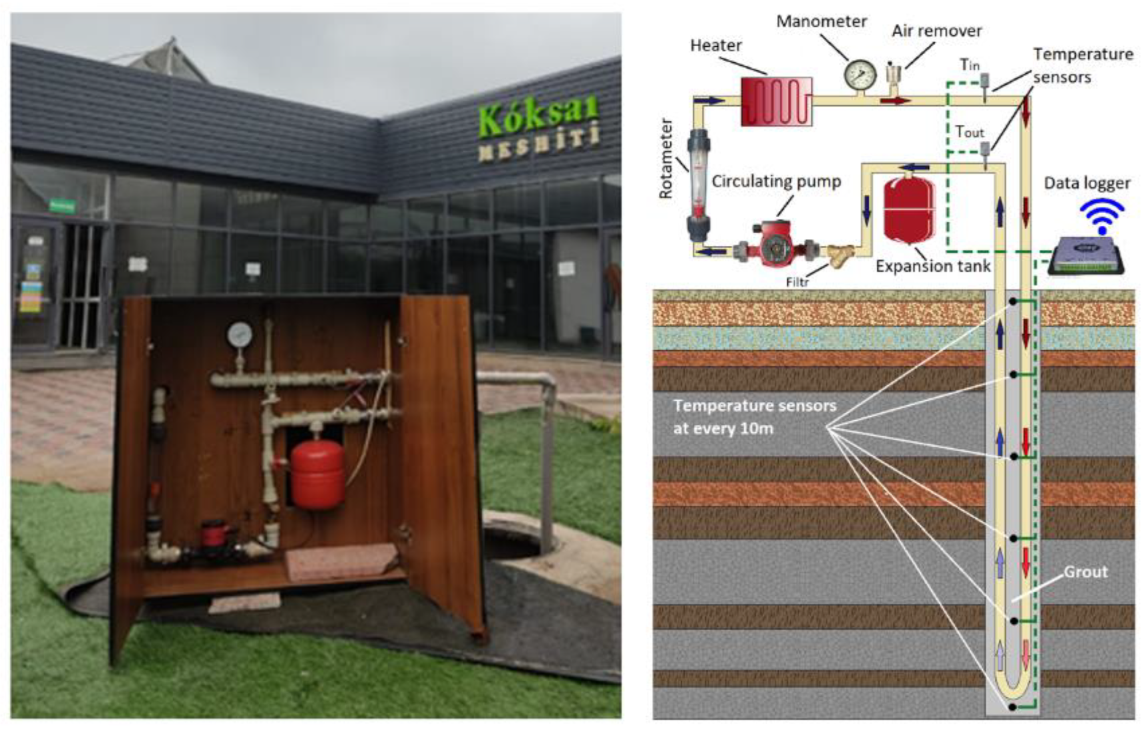
2.1. TRT Device and Test Procedure

A key part of this study was determining parameters such as the soil thermal conductivity and thermal resistance between the circulating fluid and the borehole wall. This is also essential for construction of systems such as a GSHP and borehole thermal energy storage (BTES). These parameters make it possible to correctly evaluate the thermal performance of the BHE and the thermal potential of the soil that is used as a source for GSHP and as a storage medium for BTES system. They also play a crucial role in the efficient construction of such systems on a large scale.

The first TRT device in Kazakhstan was assembled by the authors of the present research in 2015. The TRT rig consisted of elements including

• an adaptive circulating pump with 50 W power consumption, for circulating the HTF,
• a rotameter for measuring the flow rate, a heater with a power of 4.8 kW to supply constant heat flux,
• an expansion tank with a volume of 8 L to keep the pressure constant,
• ball valves for connecting and for filling the loop with the required amount of water,
• temperature sensors for measuring the temperature change over time,
• manometer for monitoring the pressure in the loop,
• air remover to prevent air trap formation in the loop, and pipes for connecting the elements in one closed loop.

All the components mentioned above were installed in a box with dimensions of 1 m × 1 m × 0.5 m (height × length × width). For data acquisition, the IDAQ data acquisition system was used, which has eight channels for measuring temperatures. The TRT rig is shown in Figure 1, and a description of the device is given in [21]. All the devices were calibrated before the start of the TRT test, more detailed characteristics and their measurement uncertainties are given in

Table A1. Thermal response test measurement device specifications.

No.	Equipment Name	Specifications
1	Temperature sensors, Pt100	Model:TS0010 Length: 1 m Class: Class C Tolerance: (0.6 + 0.008 * |t|) °C (|t| is the absolute value of the actual temperature) Electrical design: Three-wire system Probe: Temperature range: −40 °C~400 °C Material: Stainless steel Size: 4 mm × 50 mm/4 mm × 80 mm The wire: Temperature range E: −60 °C~250 °C Material: 3-Core Silver Fox Fur Jacket Teflon Insulated High Temperature Wire Net weight: 50 g
2	Rotameter, Emis Meta	Nominal diameter: 25 mm Reduced error: ± 4% Nominal medium pressure: дo 1 MPa Minimum medium pressure: 100 Pa … 1000 Pa Maximum viscosity of the medium: 5 mPa × s Medium temperature: −2 °C …+80 °C Ambient temperature: −40 °C …+70 °C Relative Humidity: no more than 95 ± 3%
3	Electrical heater, Caнгaй “УMT”	Supply voltage (three-phase): 3 × 380 ± 10 % V Supply voltage (single-phase): 3 × 380 ± 10 % V Frequency: 50 Hz Rated Power (no more): 1.6 + 3.2 kW Heated area: 48 m2 Heat transfer fluid pressure in the system: 0.25 MPa
4	Circulating Pump, Grundfos Alpha2 32–40 (180) Circulator Pump with Auto Adapt	Weight: 2.3 Kg Dimensions: 138 mm × 88 mm × 180 mm Connection Type: 2 Inch BSP Male Motor Size: 18 W Full Load Current (FLC): 0.18 A Voltage: 240 V 1 Ph 50 Hz Max Flow: 2.5 m3/h Max Head: 4 m Material: Cast Iron Impeller Material: Composite
5	Data logger, iDAQ PT-08 WiFi Data Acquisition Unit -8 Channel PT100 Thermometer Inputs	8 × 3-wire or 4-wire: PT100 thermometer Inputs Measuring range: −200° to +800 °C Converter resolution: 22 bits Interface: USB 2.0 and Wi-Fi Built-in Web-server showing data in tabular and chart display formats Configurable alarms on each channel emails sent on alarm Internal Logger Memory: 256 Kb Configurable log rate: from 5 s to 24 h Data download: in CSV or Log formats Input connectors: 2 mm Screw terminals Supply: 5VDC @ 100 m (PSU included) Operating Temperature range: 0 °C to 70 °C operating Dimensions: 92 mm × 51 mm × 18.3 mm
6	Monometer	Maximum temperature: 150 °C Maximum pressure: 1 Mпa Manometer type: analog Principle of operation: pneumatic Connection: radial Case diameter: 10 mm Accuracy class: 1.5
7	Voltage regulator	Model/series: ACH-3000/1-ЭM Input voltage range: 140–260 V Rated output voltage: 220 ± 3% Operating frequency: 50 Hz Efficiency: 97% High voltage protection (delay less than 1 s.): 220 ± 5 V Protection class: IP20 Maximum Power at Ubx ≥ 1900 V Maximum current: 15.8 A

of Appendix A.

The test procedure consists of two important steps. The first step is the measurement of the undisturbed temperature of the ground by depth. These data are used in the line source model that is discussed in the next section. There are two methods for implementing this step. The first consists of directly measuring the temperature distribution of the ground by depth using temperature sensors installed along the borehole. The calculated average temperature over the depth of the well is considered as the initial undisturbed temperature of the ground. Another method consists of measuring the temperature changes at the inlet and outlet parts of BHE. First, the circulating pump is switched on to circulate the HTF along the loop for at least 3–5 h, until the temperature variation along the borehole becomes negligible and changes at the inlet and outlet reach the same value. Then, the end value at the inlet and outlet of the BHE are considered as the reference or initial undisturbed temperature of the ground. The second step is the measurement of the temperature changes at the inlet and outlet pipes of the BHE, to extract data regarding the thermal conductivity of the ground and the thermal resistance of the borehole. To carry out this procedure, a heater is switched on, to supply constant heat to the loop and the HTF is allowed to circulate in the BHE. This test is performed for 5–7 days, until the temperature difference at the inlet and outlet pipes become constant. If the thermal conductivity of the ground is low, the average value of the temperature of the circulating fluid at the inlet and outlet sections of the BHE will rise rapidly. On the contrary, if the ground has a higher thermal conductivity, then the average value of the temperature of the circulating fluid at the inlet and outlet sections of BHE will become constant over time and the angle between average temperature and time (e.g., ln(t)) will be negligible. The difference in the temperatures of the circulating fluid and the ground also provides information about the thermal resistance of the BHE.

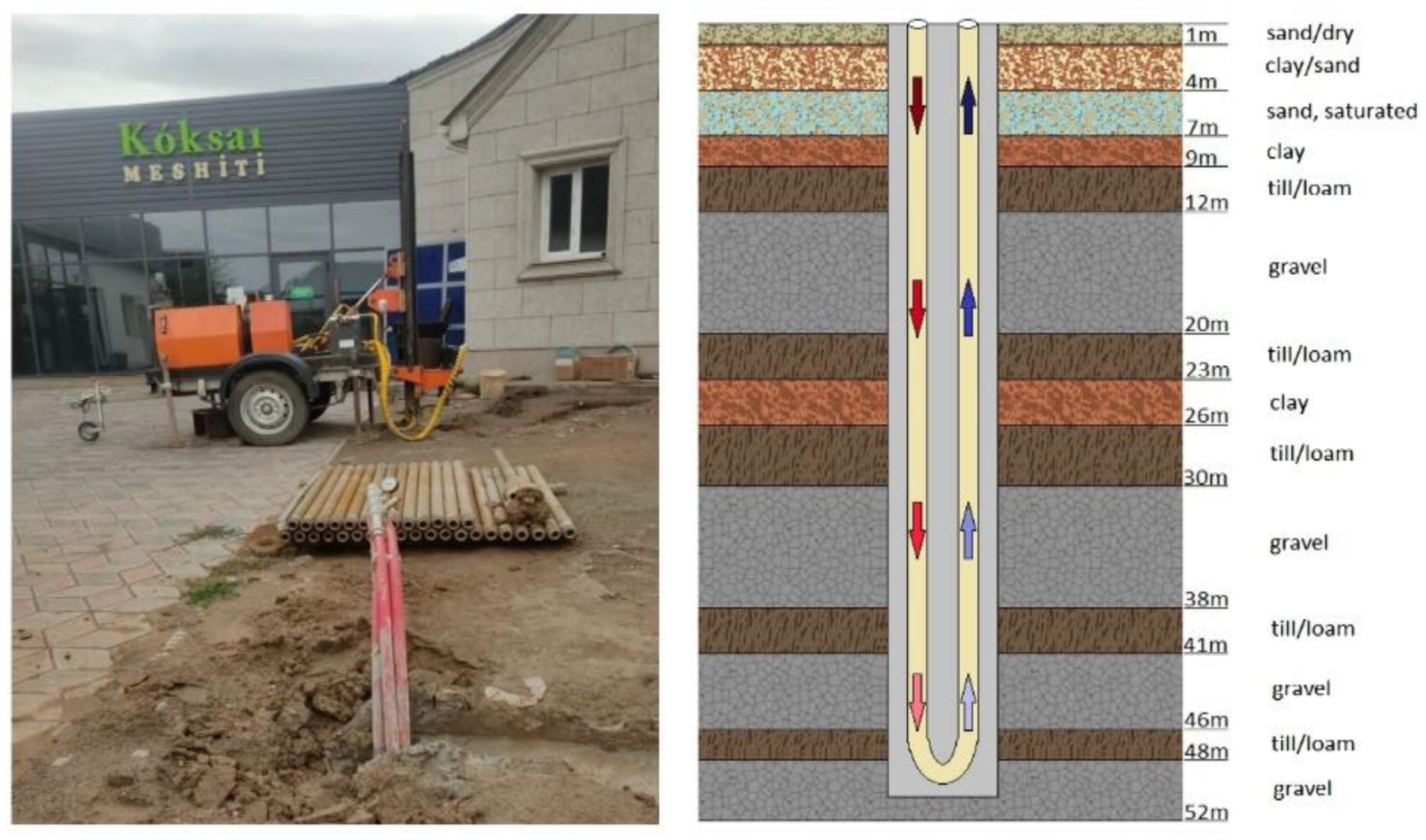
2.2. Location and Geological Structure of the Site for GSHP Construction

A prototype of the GSHP was installed at the “Koksai” mosque in the Almaty region of Kazakhstan (Karasai district, Koksai village, Arai str. 50/1). Previously, the authors of this study had installed a system of seasonal and daily solar thermal energy storage for space and water heating in this mosque. The solar thermal system was integrated into the heat pump, which allows the system to work in a solar-assisted GSHP mode. The coordinates of the site are 43°15’55.4” N 76°46’33.0” E.

Before the drilling process and construction of GSHP system, the stratigraphic map of the site (given in

Table 1. Data taken from stratigraphic map of Koksai area [62].

Formation Thickness, m	Characteristics of Rocks
180	Boulders, pebble, gravel, sand, sandy loam and till/loam
200	Boulder-pebbles, sand, loess loam, gravel
30–230	Boulder-pebbles, sand, loess loam
440–900	Middle-Upper Pliocene. Ili retinue. Pale clays, silts, sands, gravel-stones, sand-pebbles
400–1080	Red-brown mudstones with interlayers of green-gray, rubble
720	Silts, red-brown mudstones with green-gray interlayers, rubble
900–1200	Liparitic and dacitic porphyries, tuff lavas, tuffs, porphyrites, interbeds of tuff sandstones
820–1200	Katmen suite. Andesitic, andesite-basaltic porphyrites, their tuffs, dacitic porphyries and their tuffs, conglomerates, sandstones with Caenodendron primaevum Z a l., Lepidodendron cf. obovatum Sternb., Asterocalamites serobiculatus (Schloth.) Zeil.

) was studied. It was found that down to a 180 m depth, the ground consists of unconsolidated rock types such as boulders, pebble, gravel, sand, sandy loam, and till/loam. The information source originated in 1967, and the Scientific and Editorial Council of the Ministry of Geology of the Kazakh Soviet Socialist Republic approved the map in 1973 [62].

For the installation of the BHEs supplying low-grade thermal energy to the GSHP, two wells with a 50 m depth were vertically drilled. One of the wells was for installing a single U-shape BHE and the other was for installing a double-cross U-shaped heat exchanger. Drilling was carried out with a GBU-22L trailer drilling rig (see Figure 2), flush drilling type. The general technical characteristics of the drilling rig were as follows: a small-sized rig on a trailer, torque—900 N/m, rig power—22 hp, gasoline internal combustion engine—22 hp, carriage feed drive type—cylinder, drilling depth with flushing up to 100 m, and mass—750 kg. After the implementation of the descent of two heat exchangers, a gradual plugging of the space between the borehole wall and GHE with cement mortar was carried out in the ratio of 70% water, 24% cement, and 6% bentonite (see Figure 2).

During the drilling process, the geological structure of the site was found to consist of four main types of unconsolidated soil: clay, till/loam, sand, and gravel. Since Almaty is located in the foothills of the Trans-Ili (Zailiyskiy) Alatau mountains, the ground formation of the site consists of nearly 48% gravel, 29% till/loam, and 23% sand and clay. The ground formation of the site is depicted in Figure 2. The thermophysical properties of the soil layers are listed in

Table 2. Thermophysical properties of the underground soil types.

Soil Layers	Depth, m	Thermal Conductivity $\mathit{\lambda }$, W/m K [16]	Density $\mathit{\rho }$, 103 kg/m3 [19]	Volumetric Heat Capacity $\mathit{\rho }\mathit{c}$, MJ/m3 K [19]	Porosity $\mathit{\phi }$ [63]
sand, dry	0–1	0.40	2.00	1.45	0.31
sandy clay	1–4	1.60 [17]	2.10	2.45	0.35 [17]
sand, moist	4–7	1.40	2.10	2.50	0.31
clay	7–9	1.80	2.10	2.40	0.45
till/loam	9–12	2.40	2.05	2.00	0.45 [17]
gravel	12–20	1.80	2.10	2.40	0.26
till/loam	20–23	2.40	2.05	2.00	0.45 [17]
clay	23–26	1.80	2.10	2.40	0.45
till/loam	26–30	2.40 [17]	2.05	2.00	0.45 [17]
gravel	30–38	1.80	2.10	2.40	0.26
till/loam	38–41	2.40	2.05	2.00	0.45 [17]
gravel	41–46	1.80	2.10	2.40	0.26
till/loam	46–48	2.40	2.05	2.00	0.45 [17]
gravel	48–52	1.80	2.10	2.40	0.26

.

3. Solution Approaches

3.1. Analytical Solution: Line Source Model Based on Kelvin’s Theory

Analytical models, such as linear and cylindrical source models, were used to evaluate the thermal conductivity of the ground and thermal resistance of the borehole. To obtain an analytical solution and introduce some simplifications into the mathematical model of heat transfer processes between the BHE and ground, some assumptions were made: the soil was considered as an infinite homogeneous and isotropic medium; and the temperature difference between the inlet and outlet sections of the heat exchanger remained constant over time. The non-steady heat transfer problem in the system could be solved by considering the GHE as a linear heat source that continuously releases a constant amount of energy into a homogeneous medium (soil), which is unlimited in the normal direction to the axis of borehole and has a uniform initial temperature.

In this case, the length of the linear source is assumed to be sufficient to neglect the heat transfer along the borehole axis. The resulting mathematical model is given by the following heat conduction equation:

$$\frac{{\partial }^{2}T}{\partial x^2}+\frac{{\partial }^{2}T}{\partial y^2}+\frac{{\partial }^{2}T}{\partial z^2}=\frac{1}{{\alpha }_g}\frac{\partial T}{\partial t},$$

(1)

where ${\alpha }_g$ is the thermal diffusivity of the ground. The processes of convective heat transfer due to the presence of groundwater are not considered in the model. The solution of Equation (1) is given in [35,64] as:

$$\mathrm{T}\left(r,t\right)={\mathrm{T}}_0+\frac{q}{4\pi {\lambda }_g}{{\displaystyle \int }}_{\frac{r^2}{4\alpha t}}^{\infty }\frac{e^{-u}}{u}du={\mathrm{T}}_0-\frac{q}{4\pi {\lambda }_g}\mathrm{Ei}\left(-\frac{r^2}{4{\alpha }_{g}t}\right),$$

(2)

where ${\mathrm{T}}_0$ is the undisturbed reference ground temperature. The exponential function $\mathrm{Ei}$ is given by:

$$-\mathrm{Ei}\left(-x\right)={{\displaystyle \int }}_x^{\infty }\frac{e^{-u}}{u}du,$$

(3)

where $x=\frac{r^2}{4{\alpha }_{g}t}$ has no elementary analytic expression. However, $\mathrm{Ei}\left(-x\right)$ can be expanded in a series for small values of x as:

$$\mathrm{Ei}\left(-x\right)=\gamma +\ln x-x+\frac{1}{4}{x}^2+\mathrm{O}\left(x^3\right),$$

(4)

where $\gamma =0.5772$ is Euler’s constant. This expansion has a 2% accuracy under the condition $\frac{r^2}{4{\alpha }_{g}t}\ge 20$, and a 10% accuracy if $\frac{r^2}{4{\alpha }_{g}t}\ge 5$. Consequently, after substituting Equation (4) in Equation (2), the change in the temperature field for large value of $t$ reads:

$$\mathrm{T}\left(r,t\right)={\mathrm{T}}_0+\frac{q}{4\pi {\lambda }_g}\left(\ln \left(\frac{4{\alpha }_{g}t}{r^2}\right)-\gamma \right).$$

(5)

In 1983, Mogensen [22] suggested a method based on the line source model that allows determining the thermal conductivity of the ground and thermal resistance of a BHE from experimental data. Nowadays, this method remains a common way of determining the thermophysical properties of the ground and BHE. If the total thermal resistance between the circulating fluid and borehole wall is expressed as $R_b=\left(T_f-T_b\right)/q$ and $T\left(r=r_b,t\right)=T_b$ then Equation (5) can be transformed as:

$$T_f={\mathrm{T}}_0+\frac{q}{4\pi {\lambda }_g}\left(\ln \left(\frac{4{\alpha }_{g}t}{r^2}\right)-\gamma \right)+R_{b}q,$$

(6)

where $T_f$ is the arithmetic mean temperature of the inlet and outlet temperatures of the BHE.

After a simple mathematical transformation, Equation (6) can be written as:

$$T_f=k\ln \left(t\right)+m,$$

(7)

where

$$k=\frac{q}{4\pi {\lambda }_g}\mathrm{and}m={\mathrm{T}}_0+\frac{q}{4\pi {\lambda }_g}\left(\ln \left(\frac{4{\alpha }_g}{r^2}\right)-\gamma \right)+R_{b}q.$$

(8)

In Equations (2), (5), (6) and (8), the thermal conductivity of the ground ${\lambda }_g$ and thermal resistance of the borehole $R_b$ were obtained from the TRT data.

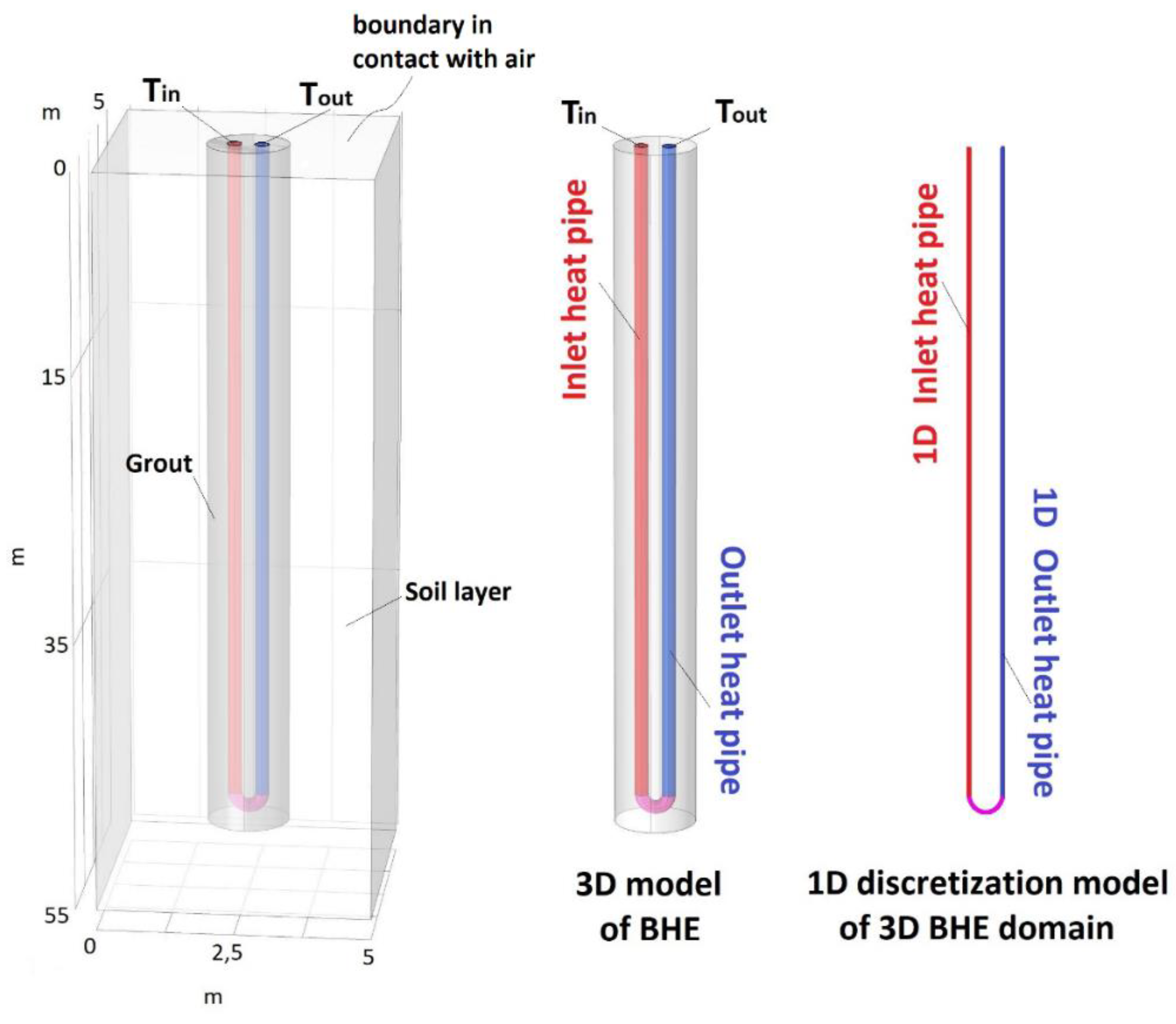
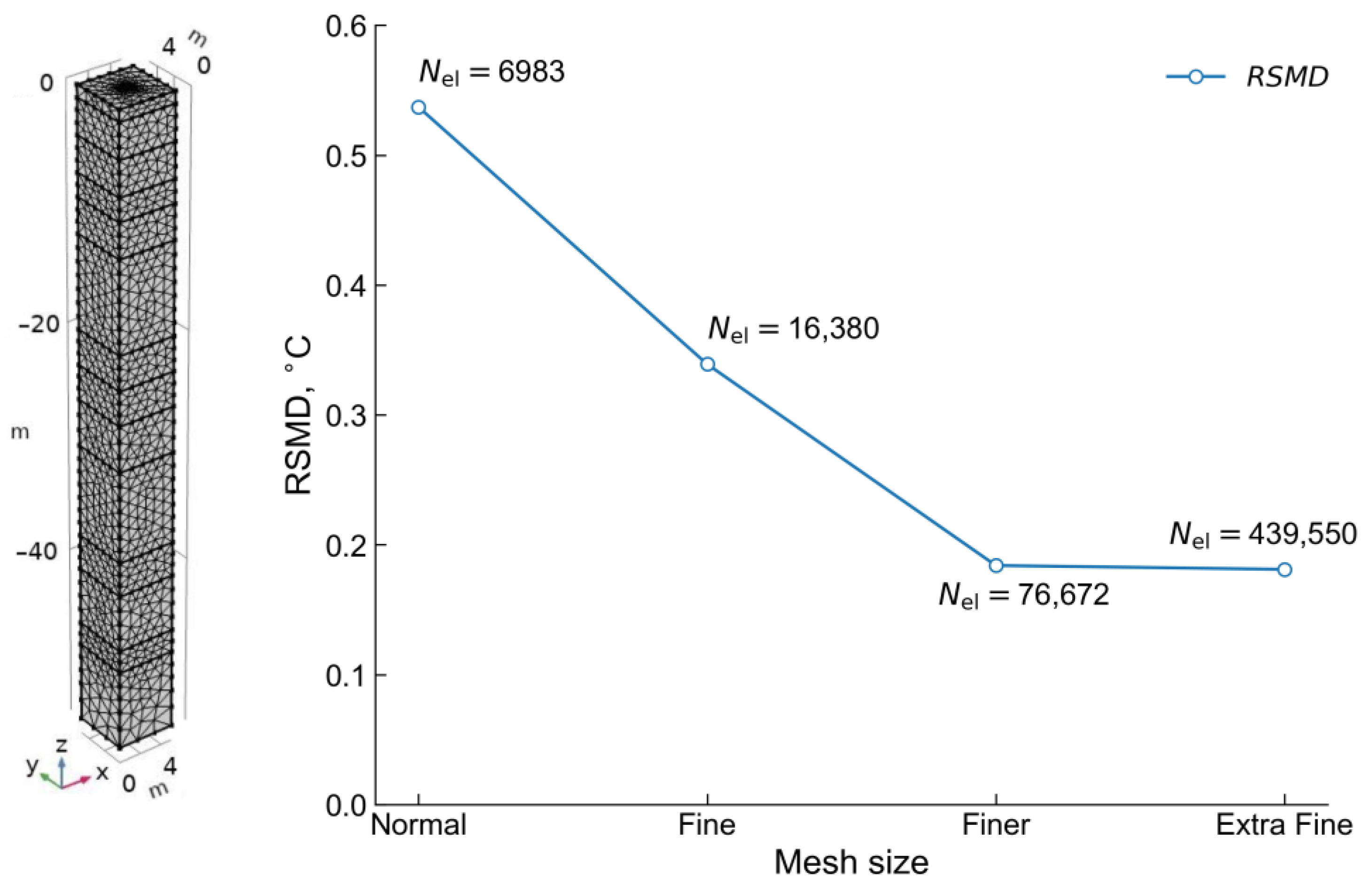
3.2. Numerical Simulation Procedure

In our physical formulation, the underground soil layers are considered to be a 3D porous medium. Figure 3 shows a 3D reservoir with finite dimensions, which was cut from shallow geothermal resources of infinite size. The length and width of the reservoir are both 5 m, and the depth is 55 m. Inside this reservoir there is a well with a diameter of 190 mm and a depth of 50 m, where a U-shaped heat exchanger with a pipe diameter of 32 mm is immersed. As mentioned above, after the U-tube is immersed, the empty space in the well is filled with cement slurry with bentonite, which is called grout. The U-shaped heat exchanger has inlet and outlet pipes, as shown in Figure 3, with corresponding HTF temperatures of $T_{in}$ and $T_{out}$. The HTF flow through the BHE pipes are based on a system of 1D equations (Figure 3), which will be described below.

Numerical simulation allows evaluating in detail the processes of heat transfer between the pipes and soil mass and identifying the key parameters that affect the performance characteristics of the BHE. It also significantly reduces the financial costs and time required for conducting real experiments. Therefore, an adequate mathematical model is needed for such a numerical analysis. During numerical simulation of geothermal systems, a unique problem arises, due to the disproportionality of the borehole heat exchanger geometry. Since the ratio of the pipe’s diameter to its length is about 1/5000, consideration of a 3D grid would lead to unreasonable computational costs. As an alternative, we consider a 1D model of heat and mass transfer for HTF in U-shaped pipes. As stated above, the 3D reservoir is a “piece of cake” carved out of shallow geothermal resources, and the soil layers are considered as porous media (see Figure 3). To simulate heat and mass transfer processes in a porous medium, a 3D model is used that considers the soil layers, porosity, moisture content, and other soil properties.

3.3. Mathematical Formulation

Ground water flow in a porous medium: the main equations of heat and mass transfer in a porous medium are the mass conservation equation, Darcy’s law, and the energy balance equation. Soil is a porous medium, which is a complex three-phase system consisting of a solid phase, a liquid phase, and air. Groundwater flow in such systems occurs through communicating pores due to a pressure drop. The filtration process is described by the mass conservation equation:

$$\frac{\partial \rho }{\partial t}+div\left(\rho \overrightarrow{v}\right)=0$$

(9)

and with Darcy’s law:

$$\overrightarrow{v}=-Kgradh,$$

(10)

where $\overrightarrow{v}$ is the groundwater flow velocity vector, $K$ is hydraulic conductivity, and $h$ is the hydraulic head.

The boundary conditions are

$$h\left(x=0,y,z\right)=h_1\hspace{1em}\hspace{1em}\hspace{1em}\mathrm{at}\mathrm{the}\mathrm{surface}x=0,$$

(11)

$$h\left(x=l_x,y,z\right)=h_2\hspace{1em}\hspace{1em}\hspace{1em}\mathrm{at}\mathrm{the}\mathrm{surface}x=l_x,$$

(12)

$$K\nabla h\overrightarrow{n}=0\hspace{1em}\hspace{1em}\hspace{1em}\hspace{1em}\mathrm{all}\mathrm{other}\mathrm{boundaries}.$$

(13)

Heat flow in a porous medium: heat transfer in a porous medium occurs due to the thermal interaction between the BHE and the soil. As the HTF charges/discharge heat to/from the surrounding soil mass during the GSHP operation, a temperature difference appears in the soil layers along the well and around the BHE, causing a heat flow from high to low temperature points. In the presence of a groundwater flow, heat is transferred from one point to another by means of conduction and convection. Hence, a convective term is added to the non-steady state heat conduction equation, which reads:

$${(\rho c)}_{eff}\frac{\partial T_s}{\partial t}dV+{(\rho c)}_f\overrightarrow{v}\cdot \nabla T_{s}dV=\nabla \cdot \left({\lambda }_{eff}\nabla T_s\right)dV+H,$$

(14)

where $T_s$ is the soil temperature and$H$is the heat source. The effective thermal conductivity ${\lambda }_{eff}$ and volumetric heat capacity ${(\rho c)}_{eff}$ in a porous medium are given by:

$${\lambda }_{eff}=\left(1-\phi \right){\lambda }_s+\phi {\lambda }_f,$$

(15)

$${(\rho c)}_{eff}=\left(1-\phi \right){(\rho c)}_s+\phi {(\rho c)}_f,$$

(16)

where $\phi$is the porosity, and the subscripts $s$ and $f$ refer to the ground and the ground water, respectively.

The initial condition is given by the undisturbed temperature of the underground soil layers:

$$T_s\left(x,y,z,t=0\right)=T_{initial}\left(z\right).$$

(17)

Boundary conditions:

The numerical solution is more accurate when using the Dirichlet boundary condition at the boundary faces of the reservoir. However, in this case, the temperature distribution near the well can affect the boundary temperatures of the reservoir. To do this, it would be necessary to increase the size of the computational domain (to at least 30 m diameter), leading to an unreasonably large computational time. In order to reduce the computational time, Neumann boundary conditions are used at all faces of the reservoir, except for the top face in contact with the atmospheric air, leading to the following conditions:

$${\lambda }_{eff}\nabla T\overrightarrow{n}=U_{as}\left(T_a-T_s\right)\mathrm{on}\mathrm{the}\mathrm{boundary}\mathrm{in}\mathrm{contact}\mathrm{with}\mathrm{the}\mathrm{air},$$

(18)

$${\lambda }_{eff}\nabla T\overrightarrow{n}=0\hspace{1em}\hspace{1em}\hspace{1em}\mathrm{Neumann}\mathrm{boundary}\mathrm{condition}.$$

(19)

Heat transfer processes in BHE: water is circulated in the heat exchanger pipes using a circulation pump and, after switching on the heater, the water temperature begins to rise gradually, resulting in a temperature difference between the components of the BHE and the surrounding soil mass, which leads to heat transfer between them. It should be noted that heat in liquids is transferred in a convective manner through their cross-sectional area. At the same time, the heat flow between the liquid and grout occurs through their surface area. The direct heat transfer between the two inlet and outlet pipes was not considered, since heat transfer between them occurs through the grout, where the grout behaves as an intermediate medium, transferring heat from the pipes to the porous medium.

Heat transfer fluid flow in BHE: to calculate the flow velocity and pressure, the flow is considered as fully developed, shocks are neglected, velocity components normal to the axis of the pipe are assumed to be 0, and the empirical correlations describing the viscous pressure drop are valid for both laminar and turbulent flow regimes. The fluid flow velocity and pressure in the heat exchanger are described by continuity and momentum equations and are expressed as follows:

$${\rho }_f\frac{\partial u}{\partial t}=-{\nabla }_{t}p\cdot {\overrightarrow{e}}_t-\frac{1}{2}f\frac{{\rho }_f}{d_p}u\left|u\right|+\overrightarrow{F}\cdot {\overrightarrow{e}}_t,$$

(20)

$$\frac{\partial A{\rho }_f}{\partial t}+{\nabla }_t\cdot \left(A{\rho }_{f}u{\overrightarrow{e}}_t\right)=0,$$

(21)

where $u$ is the tangential velocity, ${\overrightarrow{e}}_t$ is the unit tangent vector to the pipe axis, ${\rho }_{f }$ is the fluid density, $p$ is the pressure, $f$ is the Darcy friction factor, $\overrightarrow{F }$ is the volume force, $d_p$is the diameter of the heat exchanger pipes, and the second term on the right-hand side of Equation (20) represents the pressure drop due to viscous shear.

Initial conditions:

$$u\left(z,t=0\right)=0.$$

(22)

Boundary conditions:

$$u\left(z=0,t\right)=0.2m/s,$$

(23)

$$\frac{\partial u\left(z=l,t\right)}{\partial z}=0.$$

(24)

Heat transfer in BHE: considering all the above heat transfer mechanisms, the conductive–convective heat transfer between the BHE and the soil, as well as between the components of the borehole heat exchanger is expressed as:

$${\rho }_{f}A{c}_f\frac{\partial T_f}{\partial t}+{\rho }_{f}A{c}_{f}u\overrightarrow{e}\cdot {\nabla }_t{T}_f={\nabla }_t\cdot A{\lambda }_f{\nabla }_t{T}_f+\frac{1}{2}f\frac{{\rho }_{f}A}{2d_p}\left|u\right|u^2+q_{wall},$$

(25)

where ${\rho }_{f }$ is the fluid density; $A$ is the pipe cross-section area; $c_f$ is the specific heat capacity at constant pressure; $T_f$ is the fluid temperature, where $u$ is tangential velocity; ${\overrightarrow{e}}_t$ is unit tangent vector to the pipe axis; ${\lambda }_f$ is the thermal conductivity; $d_p$ is the diameter of the heat exchanger pipes; and the second term on the right-hand side of Equation (25) is the friction heat dissipated due to viscous shear. $q_{wall}$ is the radial heat transfer from the surrounding soil into the heat exchanger pipes, which is expressed as:

$$q_{wall}={(\tilde{h}Z)}_{eff}\left(T_{ext}-T\right),$$

(26)

where ${(\tilde{h}Z)}_{eff}$ is the effective value of heat transfer coefficient, $\tilde{h}$ is the heat transfer coefficient, $Z=2\pi r_{p,in}$ is the inner perimeter of heat exchanger pipes, and $T_{ext}$ is the external temperature outside the pipe (grout temperature). The expression of ${(\tilde{h}Z)}_{eff }$is given by:

$${(\tilde{h}Z)}_{eff}=\frac{2\pi }{\left(\frac{1}{r_{p,in}{\tilde{h}}_{int}}+\frac{\ln \left(r_{p,out}/r_{p,in}\right)}{{\lambda }_p}\right)},$$

(27)

where $r_{p,in}$ and $r_{p,out}$ are the inner and outer radius of pipes, ${\lambda }_p$ is the thermal conductivity of the pipe wall material, and${\widetilde{ h}}_{int}$ is the heat-transfer coefficient of the HTF inside pipes, given by Equation (28):

$${\tilde{h}}_{int}=Nu\frac{{\lambda }_f}{d_p},$$

(28)

Nu can be calculated using the Gnielinski equation [65], as given by Equation (29):

$$Nu=\frac{\left(f/8\right)\left(\mathrm{Re}-1000\right)Pr}{1+12.7{\left(f/8\right)}^{1/2}\left({\mathrm{Pr}}^{2/3}-1\right)},$$

(29)

where$f$is the Darcy friction factor, $Re$ is the Reynolds, and $\mathrm{Re}=\frac{{\rho }_{f}u{d}_p}{{\mu }_f}$ and $Pr$are the Prandtl numbers, $\mathrm{Pr}=\frac{c_f{\mu }_f}{{\lambda }_f}$. For the flow of single-phase fluids, $f$ can be determined using the Churchill equation [66], as given by Equation (30):

$$f=8{\left[{\left(\frac{8}{Re}\right)}^{12}+{\left(\tilde{A}+\tilde{B}\right)}^{-1.5}\right]}^{1/12},$$

(30)

where

$$\tilde{A}={\left[-2.457\ln \left({\left(\frac{7}{Re}\right)}^{0.9}+0.27\left(e/d\right)\right)\right]}^{16},$$

(31)

$$\tilde{B}={\left(\frac{37530}{Re}\right)}^{16}.$$

(32)

where $e/d_p$ is the relative surface roughness of the inner wall surface of the pipe.

Equation (29) covers the whole range of laminar, transition, and turbulent flows and is valid for the wide ranges of 3000 < $Re$ < 6 × 10⁶ and 0.5 < $Pr$ <2000.

Initial conditions:

$$T_f\left(z,t=0\right)=T_{initial}\left(z\right),$$

(33)

where $T_{initial}\left(z\right)$ is the undisturbed soil temperature.

Boundary conditions:

$$T_f\left(z=0,t\right)=T_{in}\left(t\right),$$

(34)

$$\frac{\partial T_f\left(z=l,t\right)}{\partial z}=0.$$

(35)

4. Results and Discussions

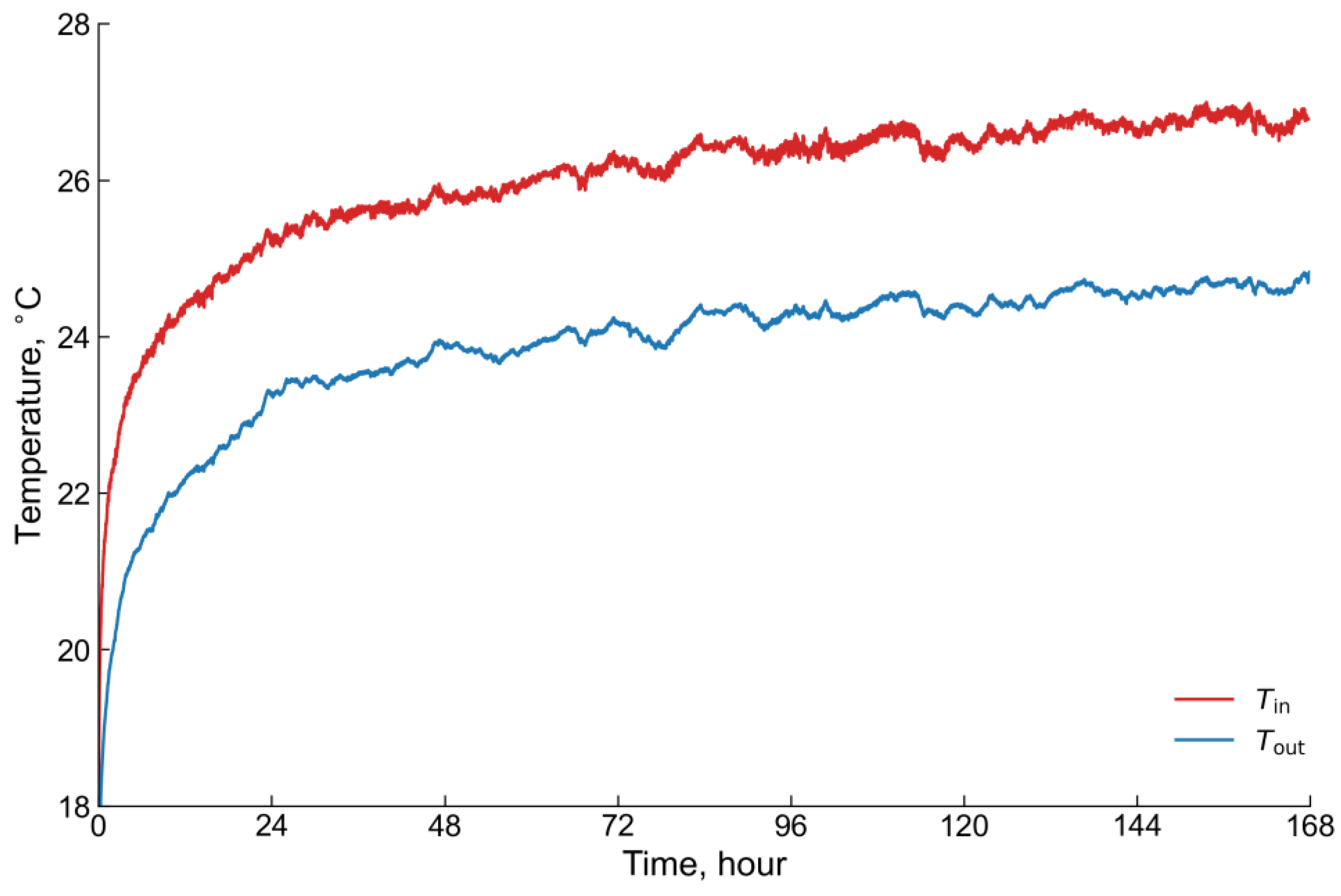
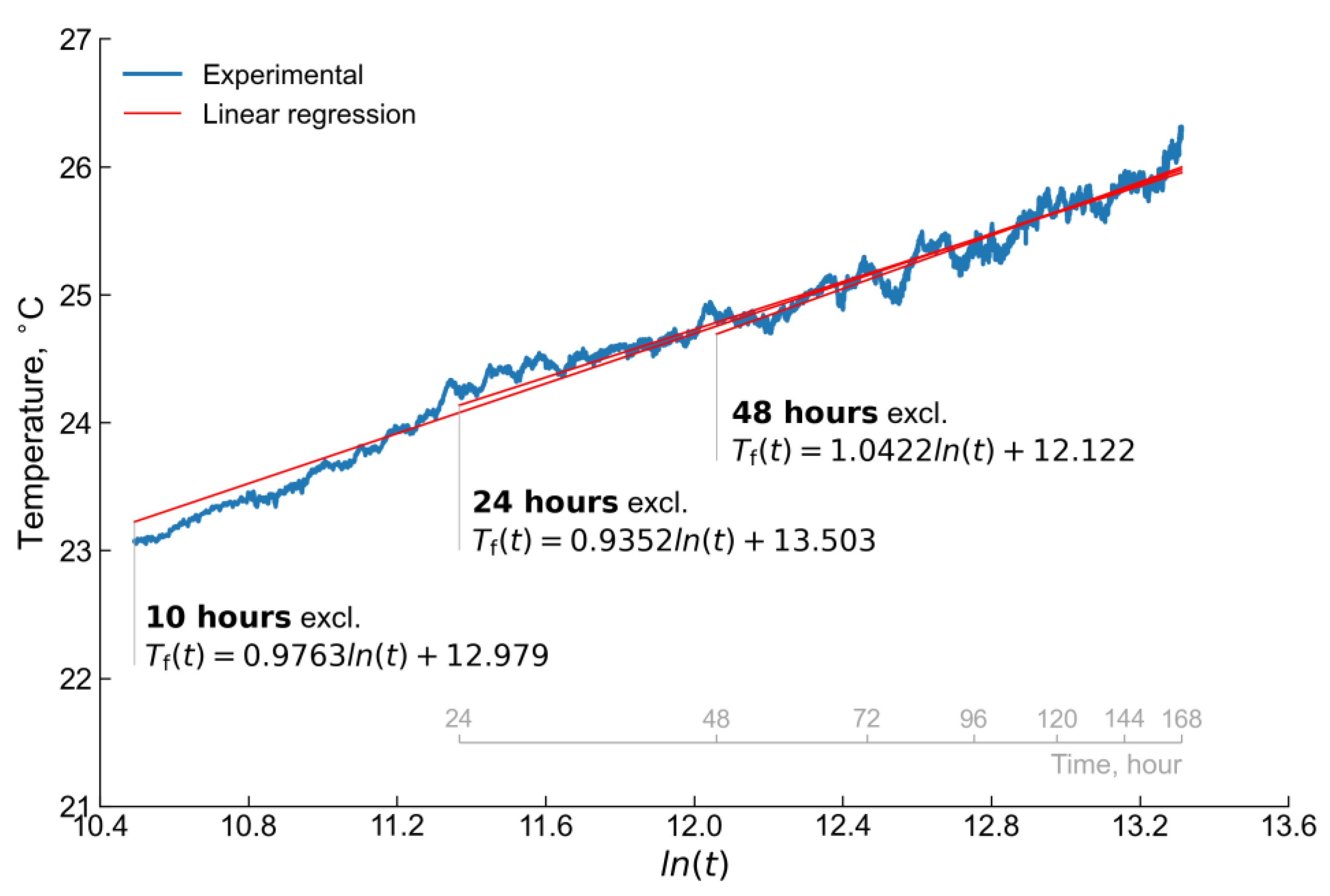
4.1. TRT Test Results

Figure 4 shows a graph of the temperature change over time for the HTF at the inlet and outlet parts of the single U-shaped BHE according to the TRT experimental results. In this figure, $T_{in}$ is the temperature of the injected heat with constant support of the electric heater, while $T_{out}$ is the temperature of the cooled HTF after transferring heat to the ground. The temperatures $T_{in}$ and $T_{out}$ were measured at the inlet and outlet of the U-shaped heat exchanger (on the ground surface) for the HTF. As shown in Figure 4, a small angle existed between the temperature profiles and the abscissa of the coordinate system (after one day). This angle is an indicator of the difference in thermal conductivity between the ground and grout. As seen in Figure 4, both the grout and the ground have good thermal conductivity, which produced the indicated small angle. In the seven days of the experiment, $T_{in}$ was 27.21 °C and $T_{out}$ was 25.23 °C, so the average difference between them was 2.10 ℃.

Figure 5 shows the experimental results of the initial distribution of soil temperature over the depth of the well, as measured by the five sensors installed along the BHE (see Figure 1), which were installed at depths of 1 m, 10 m, 20 m, 30 m, 40 m, and 50 m. The shape of the temperature distribution is similar to the results of other studies [19,20]. Down to a depth of 15 m, the effect of seasonal fluctuations in atmospheric air temperature is visible, with measurements taken in June 2022. Further down, from 15 m to 50 m, the average ground temperature was 15.0 °C.

Figure 6 is a plot of the undisturbed reference soil temperature versus time, which was obtained using an alternative method. This alternative method consisted of determining the temperature of the soil before heat injection, which was carried out with the temperature values $T_{in}$ and $T_{out}$. This was achieved by long-term circulation of the HTF until a thermal balance was reached between the fluid in the heat exchanger pipes and the soil. It appeared that after 11 h the average temperatures of $T_{in}$ and $T_{out}$ were 14.5 °C. During the operation of the circulation pump, heat is released, the influence of which was insignificant for the experiment, therefore this heat was not considered when determining the undisturbed soil temperature. The difference between the average temperatures of the undisturbed soil obtained by the first and second methods was only 0.5 ℃. Since direct measurement is considered more accurate, 15.0 °C was used as the average undisturbed soil temperature for the line-source model when determining the BHE thermal resistance.

Figure 7 shows a plot of the heat transfer rate versus time, where the heat transfer rate was supplied using an electric heater. The influence of ambient air heat was not considered since the pipes on the ground surface were well insulated and heat was supplied only by the electric heater. The amount of thermal energy obtained from the electric heater was calculated using a basic thermodynamic formula from the measurements of $T_{in}$ and $T_{out}$. As seen in Figure 7, the average power of electric heater was 1.48 kW for 50 m, which is equivalent to 30 W/m.

Figure 8 shows a graph of the temperature change according to Equation (7) of the analytical model for determining the thermal conductivity of the soil and BHE thermal resistance. In this case, the temperature $T_f$ can be understood as the arithmetic average between $T_{in}$ and $T_{out}$ (blue solid line). According to the coefficients $k$ and $m$ obtained through linear regression, the thermal conductivity $\lambda$ and the thermal resistance $R_b$ were determined by Equation (8).

Figure 9 shows plots of $T_f$ as a function of time with various exclusions of the initial time intervals, to eliminate initial perturbations of the experimental data. The results obtained with the various coefficients $k$ and $m$ used in Figure 9 were then inserted into Equation (8). The results of these calculations are presented in

Table 3. Results of the analytical model.

Time	Slope k	$\mathit{m}$	$\mathit{Q}$ BHE (W)	${\mathit{\lambda }}_{\mathit{g}}$ (W/m K)	${\mathit{R}}_{\mathit{b}}$ (m K/W)
Overall	1.03	12.313	1470	2.2720	0.1929
10 h	0.98	12.979	1470	2.3879	0.2016
1st day	0.94	13.503	1470	2.4895	0.2082
2nd day	1.04	12.122	1470	2.2501	0.1891
Mean	-	-	-	2.35	0.20

.

Based on the results of Table 3, the following values of thermal conductivity and thermal resistance were obtained: ${\lambda }_g$ = 2.35 W/m K and $R_b$ = 0.20 m K/W. These values, which are comparable with the results of other studies [19,20], were used in the numerical model described in Section 4.2.

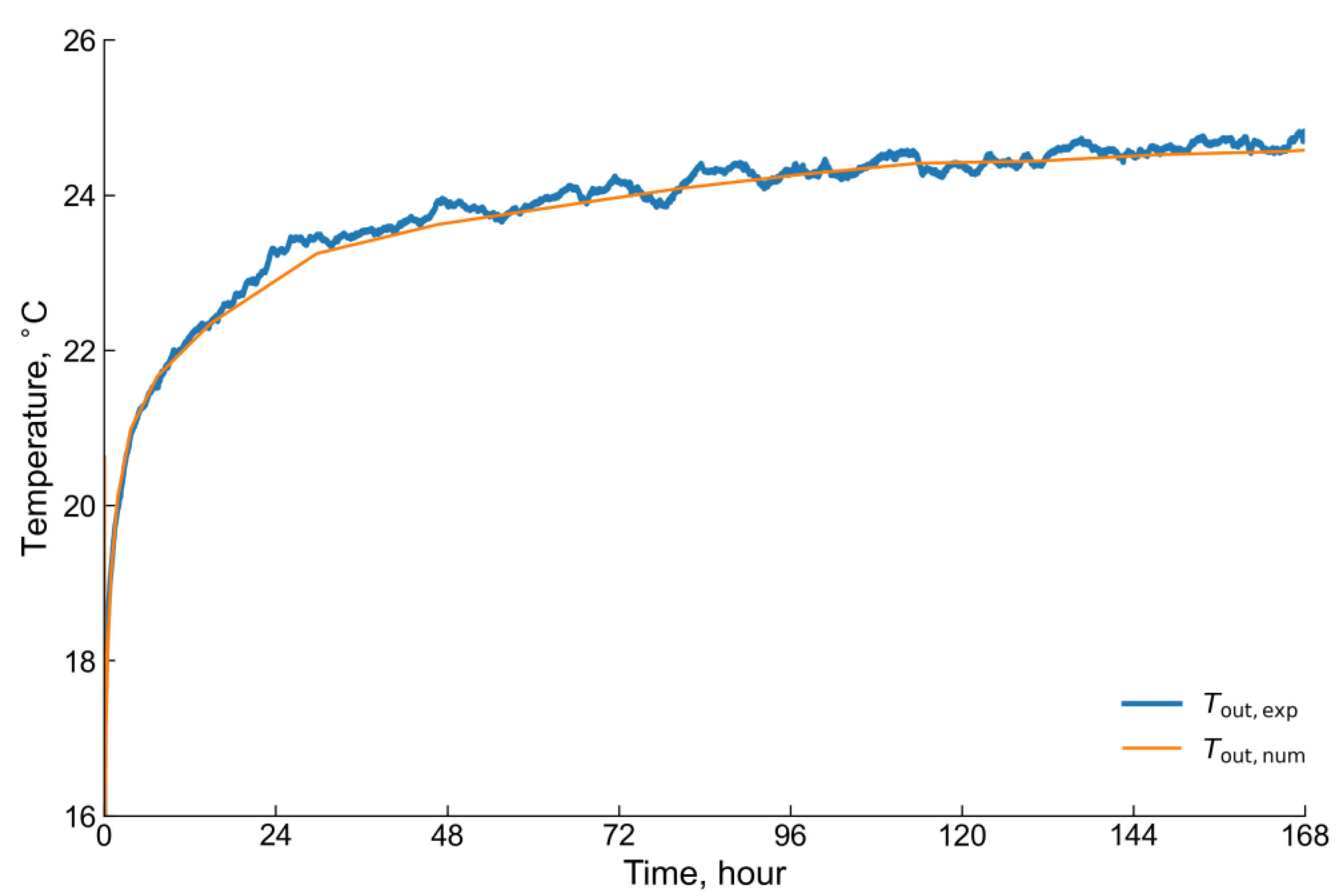
4.2. Numerical Model Verification

For the numerical implementation of the mathematical model (9)–(34), COMSOL Multiphysics software was used with solvers for heat and mass transfer in a porous medium (9)–(19), fluid flow in the BHE (20)–(24), and the heat transfer between the working fluid in the BHE and the surrounding soil (25)–(34). To verify our mathematical modelling with COMSOL, the numerical solution of a single U-shaped heat exchanger was calculated and compared with the experimental data obtained from the TRT tests. Figure 10 compares the numerical and experimental results with the experimental data for the temporal evolution of $T_{out}$. This figure illustrates the validity of our numerical modelling, since the numerical results accurately fit the experimental data, with a $RMSD$ = 0.184 °C.

Figure 11 shows a comparison of the simulation results with different grids. Four different computational grids were adopted: normal—6983 elements, fine—16,380 elements, finer—76,672 elements, and extra fine—439,550 elements. These computational grids were generated automatically using the COMSOL Multiphysics software for the constructed geometry of a single U-shaped heat exchanger 50 m deep. As shown in Figure 11, the most suitable size was the 76,672 element mesh. The difference in $RMSD$ of the results obtained between 76,672 and 439,550 elements was small, so the grid with 76,672 elements was adopted for the numerical simulations in Section 4.3.

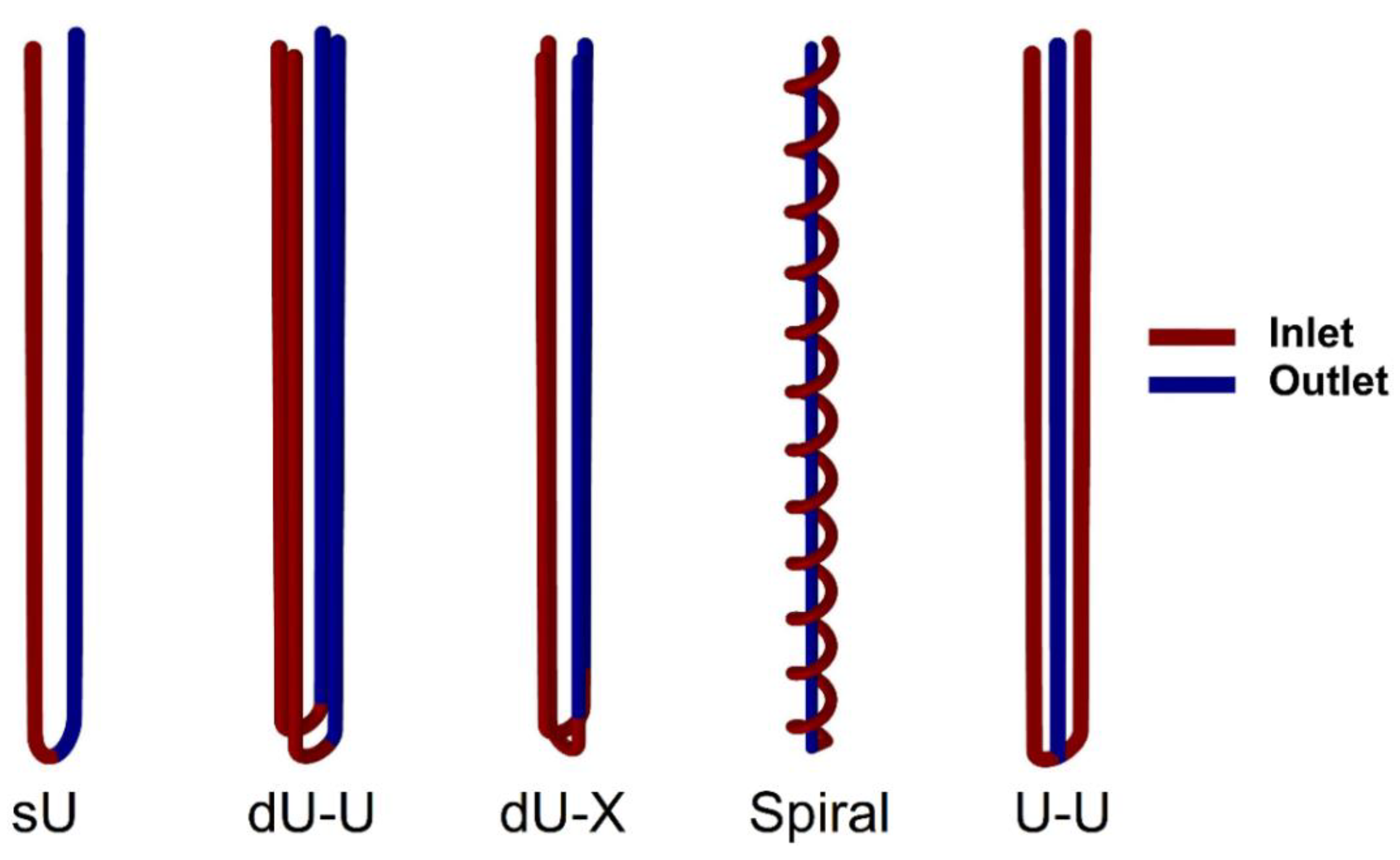
4.3. Results for BHE with Different Geometrics

In addition, numerical simulations were carried out based on a verified model for various heat exchanger pipe geometric configurations inside the BHE. Figure 12 shows the pipe configurations considered. In Figure 12, the BHEs are named with their respective pipe laying: single U-shaped (sU), double parallel (dU-U), cross (dU-X) U-shaped, spiral/helix (Spiral), and multitube (U-U) U-shaped. In all configurations, the inlet pipe is represented in red and the outlet pipe in blue. The main purpose of considering various geometries of the stacking of the pipes was to identify the most efficient configuration of the GHE, and which yielded the maximum heat exchange with the ground. For the case of a GSHP application, it is important to maximize the heat removal from the ground. In addition to the layout of the pipes, the composition of the grout, the pipe material, and the HTF flow modes should be considered as parameters of the BHE. Of course, it is also necessary to consider the thermal conductivity of the soil surrounding the BHE.

Table 4. Borehole parameters and thermal properties of the 3D calculation.

Parameters	Values
Borehole size
Borehole depth (sU)	50 m
Borehole radius	0.08 m
Inner radius of pipe	0.028 m
Outer radius of pipe	0.032 m
Half of the U-tube shank spacing (for sU, dU-U, dU-X)	0.1 m
Helix coil radius (Spiral)	0.06 m
Helix pitch (Spiral)	0.1 m
Thermal conductivity of pipe	0.4 W/(m K)
Working fluid properties
Fluid type	Water
Specific heat capacity of fluid	4183 J/(kg K)
Density of circulating fluid	997 kg/m3
Thermal conductivity fluid	0.5947 W/(m K)
Dynamic viscosity of fluid	0.0008905 kg/(m s)
Fluid flow rate	0.6 (m3/h)
Inlet fluid temperature (charging)	50 °C
Inlet fluid temperature (discharging)	5 °C
Grout thermal properties
Specific heat capacity of grout	1000 J/(kg K)
Density of the grout	2800 kg/m3
Thermal conductivity of the grout	1.7 W/(m K)
Soil thermal properties
Specific heat capacity of soil	1200 J/(kg K)
Density of soil	2500 kg/m3
Thermal conductivity of the soil	1.75 W/(m K)
Porosity of the soil	0.36
Undisturbed ground temperature	15 °C

presents the main input values for the BHE parameters and the thermal properties of materials for 3D simulations with complex geometry. For each geometrical configuration, Figure 13, Figure 14 and Figure 15 show the effects of the well depth, pipe heat exchange surface area, and heat flux given by the computations. During the analysis, one of these three parameters was fixed, and the two others were allowed to vary, while all other parameters and thermal properties from Table 4 remained unchanged. Figure 15, Figure 16, Figure 17 and Figure 18 analyze the influences of thermal properties, such as the thermal conductivities of the soil/grout/pipe materials, as well as the HTF flow rate, on the thermal performance of a single configuration: a single U-shaped BHE.

Figure 13 shows the results of the simulations for various pipe configurations with the same BHE depth of 50 m. At the same time, the heat exchanger areas of these configurations are different. As shown in Figure 13, the left orange diagram shows the thermal energy charging the ground, while the right blue diagram shows the thermal energy discharging from the ground. As can be seen from Figure 13, the trend is the same in both cases. The charging mode was carried out at a temperature $T_{in}$ = 50 °C. Under a discharging mode, the temperature $T_{in}$ was equal to 5 °C. Thus, with the same well depth of 50 m and various heat exchange areas, the BHE-extracted heat (discharging) was as follows: single U-shaped $Q$ = 1.36 kW, double U-shaped parallel $Q$ = 1.58 kW, double U-shaped cross $Q$ = 1.49 kW, spiral $Q$ = 1.91 kW, and multi-tube $Q$ = 1.50 kW.

For a GSHP operation, the discharging mode is of particular interest, since the heat of the soil is extracted. Therefore, only the heat discharging mode is considered below. As can be seen from Figure 13, for double U-configurations, the heat exchange area is doubled compared to a single U-shaped BHE, but the amount of extracted heat is only 9–14% higher, with a value of 1.49 kW for dU-X and 1.58 kW for dU-U. This is explained by the fact that the HTF, when moving along the inlet pipe to the bottom of the well, extracts heat from soil, due to the temperature difference between the soil and the HTF, reaching its maximum at the bottom of the well (50 m).

Then, when rising back from the bottom to the surface, the HTF begins to lose this heat, due to the temperature difference between the outlet and inlet pipes along the depth of the well, where the grout behaves as an intermediate medium that transfers heat from one pipe to another. The amount of heat is calculated from the temperature of the HTF at the inlet $T_{in}$ and outlet $T_{out}$ of the heat exchanger pipes. In this regard, a slight increase in the extracted heat between the single and double U-shaped heat exchangers is obtained. The greatest heat extraction was obtained for the spiral heat exchanger, since the heat exchange area of the inlet pipe down to the bottom of the well was larger than the outlet pipe from the bottom to the soil surface. This means that the HTF to the bottom received the maximum amount of heat, due to vortex movements in the branches of the tube, which increased the HTF residence time, while during rising back to the ground surface, it lost less heat, due to the straight piping. When laying a spiral pipe at a depth of 50 m, the heat transfer surface area was 12.15 m² and the amount of extracted heat was 1.91 kW. Following the same principle as with the spiral configuration, the multitube version (U-U) had two inlet pipes, which increased the amount of heat extraction before the HTF passed to the well bottom, while the return was a simple straight pipe. In this case, the total heat transfer area was 15.08 m², and the amount of extracted heat was 1.50 kW. This comparison shows that, despite the larger heat transfer area of the U-U pipe, the extracted heat was lower than that for the spiral pipe, because the HTF vortex flows in the pipe’s bends enhanced the heat transfer with the surrounding soil.

Figure 14a is a plot of well depth versus pipe-laying types. For all types of pipe, the same amount of extracted heat was considered, namely $Q$ = 1350 W, which corresponded to the value obtained for a single U-shaped heat exchanger at a depth of 50 m. The other input parameters and properties are given in Table 4. The spiral configuration gave the best results, as it saves on the drilling depth. For the spiral case at $Q$ = 1350 W, the well depth was 32.7 m. At the same time, for double U-shaped configurations, the well depths were 42.7 m (dU-U) and 45.1 m (dU-X). For a multi-tube configuration (U-U), the depth was 45.4 m. In this case, savings were made on drilling the well, but the heat transfer area changed slightly compared to a 50 m depth. The sU configuration was the geometry with the shallowest drilling depth; however, the heat transfer areas for dU-U, dU-X, and U-U were higher than for sU: 17.2 m², 18.1 m², and 13.7 m², respectively. The spiral configuration saved 34.6% on drilling depth comparing to sU, but saved only 3.96% on heat transfer area, for a value of 9.7 m². Savings in drilling costs are much more preferable than savings in piping materials. Despite the advantages of the spiral configuration, we should mention that proper installation and preparation of helix branches before immersion in the well is a delicate process.

Figure 14b shows a graph of the dependence of the heat fluxes on the type of pipes laid, with the same heat transfer area, $A_{surface}$ = 10.05 m², which corresponds to a single U-shaped heat exchanger at a 50 m depth. In this figure, the depth and heat transfer rates were allowed to vary, while all other parameters/properties remained as in Table 4. As can be seen from Figure 14b, the spiral pipe had the highest amount of extracted heat $Q$ = 1.5 kW and the well depth was 41.3 m. For double-U types, the borehole depth was 25 m, with $Q$ = 0.82 kW for dU-U and $Q$ = 0.75 kW for dU-X. For a multi-tube configuration (U-U), the well depth was 34 m and $Q$ = 1.17 kW. According to the results, the spiral pipe had the largest amount of extracted heat, with a value of 0.037 kW/m, followed by U-U 0.034 kW/m, then dU-U 0.033 kW/m, dU-X 0.030 kW/m, and sU 0.027 kW/m. As mentioned above, the spiral configuration is difficult to install, so the multi-tube and double U shapes can be recommended as less labor-intensive alternative GHEs with high heat removal for GSHP applications.

Geometric parameters such as the well depth and heat transfer surface area have been investigated. In future work, we plan to conduct additional studies on the influences of the other geometric parameters indicated in Table 4. To study the influences of different geometries on the BHE thermal performance, it is better to keep thermal properties with the same values. However, for a comprehensive study of the efficiency of a BHE, in addition to geometric parameters, it is necessary to investigate the influences of the thermophysical properties. Next, the influences of the properties of the working fluid and materials on the thermal performance of BHE were studied. In the analysis presented in Figure 15, Figure 16, Figure 17 and Figure 18, a single U-shaped BHE was considered. In this case, all input data for the calculations are given Table 4.

The influences of the grout material, piping material, and HTF flow rate on the efficiency of the BHE are shown in Figure 15, Figure 16 and Figure 17, respectively. In addition to the geometric layout of pipes inside the BHE, these parameters are also important and are an integral part of the BHE. The calculations in these graphs were carried out for single U-shaped heat exchanger at 50 m depth. Figure 15 shows a graph of the amount of extracted heat using BHE versus the thermal conductivity of the grout material. As shown in Figure 15, it follows that the higher the grout thermal conductivity, the higher the amount of heat extracted. According to [19,67], the thermal conductivity ${\lambda }_{grout}$ varied from 0.5 to 3.3 W/m K. In Figure 15, the range has been arbitrarily increased to 5.0 W/m K, to show that above a value of 3.0 W/m K, the effect of this factor is negligible. When varying ${\lambda }_{grout}$, all other thermal properties in Table 4 remained unchanged, including ${\lambda }_g$, with a value of 1.75 W/m K. It follows that no matter how high the thermal conductivity of the grout, the heat transfer of the soil is limited. If the thermal conductivity of the grout is less than the thermal conductivity of the soil, then this results in a greater resistance to the heat transfer rate from the soil to the grout, so the heat flux to the HTF will decrease. Therefore, instead of grout material, in most cases, soil excavated during drilling is used as a filler in the empty space between the pipes and the well. In the case of a higher thermal conductivity of the grout than the ground, the entire heat transfer rate from the soil side with less resistance goes to the HTF. The increase in the thermal conductivity of the grout has a limit, above which it makes no sense to increase this property.

Figure 16 shows a graph of the dependence of the heat transfer rate on the thermal conductivity of the piping material. Following [19], the pipe materials are plastic and metal-plastic, due to their low cost and durability. The range of thermal conductivity ${\lambda }_p$ presented in [19] varied between 0.24 and 0.42 W/m K. Figure 16 shows that when the thermal conductivity is increased to 2.0 W/m K, the heat extraction reaches a plateau and does not change significantly. This suggests that there is no need to use more expensive materials with higher thermal conductivities. The mechanism of heat transfer between the grout and piping material is similar to the previous discussion of the heat transfer between soil and grout. Therefore, it is possible to increase the thermal conductivity up to 2.0 W/m K, to obtain higher heat transfer rates from the ground. This can be considered a basis for further research.

Figure 17 shows a graph of the dependence of the heat transfer rate on the volumetric flow rate of the HTF in the BHE. The above experiments were carried out with a volume flow rate of 0.6 m³/h. As shown in Figure 17, with an increase in the volumetric flow rate of the fluid, the heat transfer rate increases; however, above 1.0 m³/h, this change is insignificant. In this case, the thermal conductivities were taken from Table 4, where ${\lambda }_g$=1.75 W/m K, ${\lambda }_{grout}$=1.70 W/m K, and ${\lambda }_p$=0.4 W/m K. With the specified thermal properties for the sU configuration, the maximal heat extraction by the HTF did not exceed 1.37–1.43 kW. Even an increase in the flow rate of the HTF did not increase the amount of heat extracted. This means that the maximal amount of heat that transferring from the ground to the HTF is taken away by the circulating fluid and, therefore, an increase in flow rate above 1.0 m³/h does not lead to an increase in heat removal. As a conclusion, other higher soil/grout/pipe thermal conductivity values may lead to different flow rates.

Figure 18 shows a graph of the influence of the soil thermal conductivity on the heat extracted using the BHE. Other parameters and properties are indicated in Table 4. Following [19], tabular data on various thermal conductivities of the soil were considered. For example, for dry clay/silt, the thermal conductivity ${\lambda }_g$ was 0.4–1.0 W/m K, while for water-saturated gravel/stones, the thermal conductivity was 1.6–2.5 W/m K, and for quartzite, 5.0–6.0 W/m K. As can be seen from Figure 18, with an increase in the thermal conductivity of the soil, the amount of heat extracted by the BHE increases almost linearly. According to the experimental data of the TRT, the amount of heat extracted from the indicated area in the Almaty region was 1.47 kW. In Section 2.2, where the drilling depth was 50 m, it was found that the soil structure mainly consisted of till/loam and gravel. As seen in Figure 18, for such a heat transfer rate, the thermal conductivity of the soil corresponds to till/loam and saturated gravel. When designing a GHE for GSHP, it should be noted that no matter how high the thermal conductivity of the soil, the maximal amount of heat that can be extracted is limited by the BHE performance.

5. Conclusions

In this work, experimental and numerical studies of the efficiency of a vertical ground heat exchanger in relation to ground source heat pumps were carried out. A prototype ground source heat pump was designed and installed in the Koksai mosque in the Almaty region in Kazakhstan. The prototype has two ground heat exchangers as a source of low-grade thermal energy for the heat pump: a single U-shaped heat exchanger and a double U-shaped cross heat exchanger are immersed in two wells of 50 m depth. When drilling the well, the geological structure of the area was found to be mainly gravel and till/loam. A thermal response test was carried out using a single U-shaped borehole heat exchanger. The experimental data of the soil thermal response, together with the analytical approach of the line-source model, allowed determining the soil thermal conductivity and the thermal resistance of the borehole heat exchanger. A three-dimensional model was developed for the heat and mass transfer in a porous medium (both ground and grout) outside the ground heat exchanger, and a one-dimensional model was developed for the fluid flow and heat transfer in the U-shaped pipe of the ground heat exchanger. A three-dimensional model with appropriate initial and boundary conditions was solved using COMSOL Multiphysics software. The solutions of the specified software were verified by comparison of the predictions of the model with the data of the soil thermal response test. A good agreement was found between the numerical predictions and experimental data. Numerical simulations were then performed for various geometric configurations of pipes inside the borehole heat exchanger: single U-shaped, double U-shaped parallel and cross, spiral/helix, and multi-tube. The following main conclusions can be drawn:

• An energy efficient ground source heat pump system with appropriate ground heat exchangers was developed and tested.
• An apparatus and method for testing soil thermal response were developed.
• Drilling data were in accordance with the stratigraphic map of the geological exploration data.
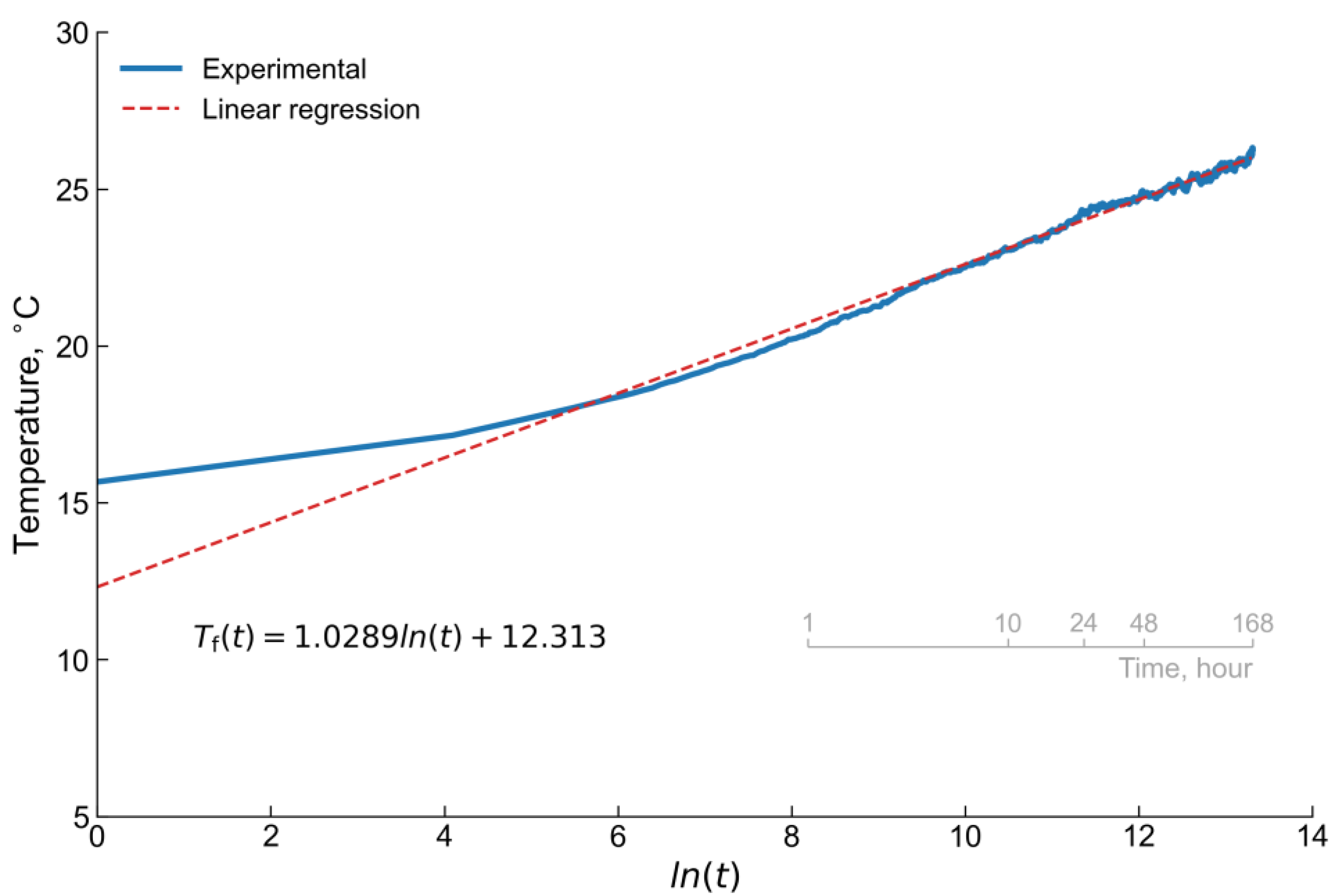
• The results of the thermal response test and the line-source analytical model showed the soil thermal conductivity was ${\lambda }_g$ = 2.35 W/m K, while the thermal resistance of the ground heat exchanger was $R_b$ = 0.20 m K/W.
• A 3D numerical tool was developed and validated with the TRT test results.
• The validation results were found to be in good agreement, with an RMSD = 0.184 °C.
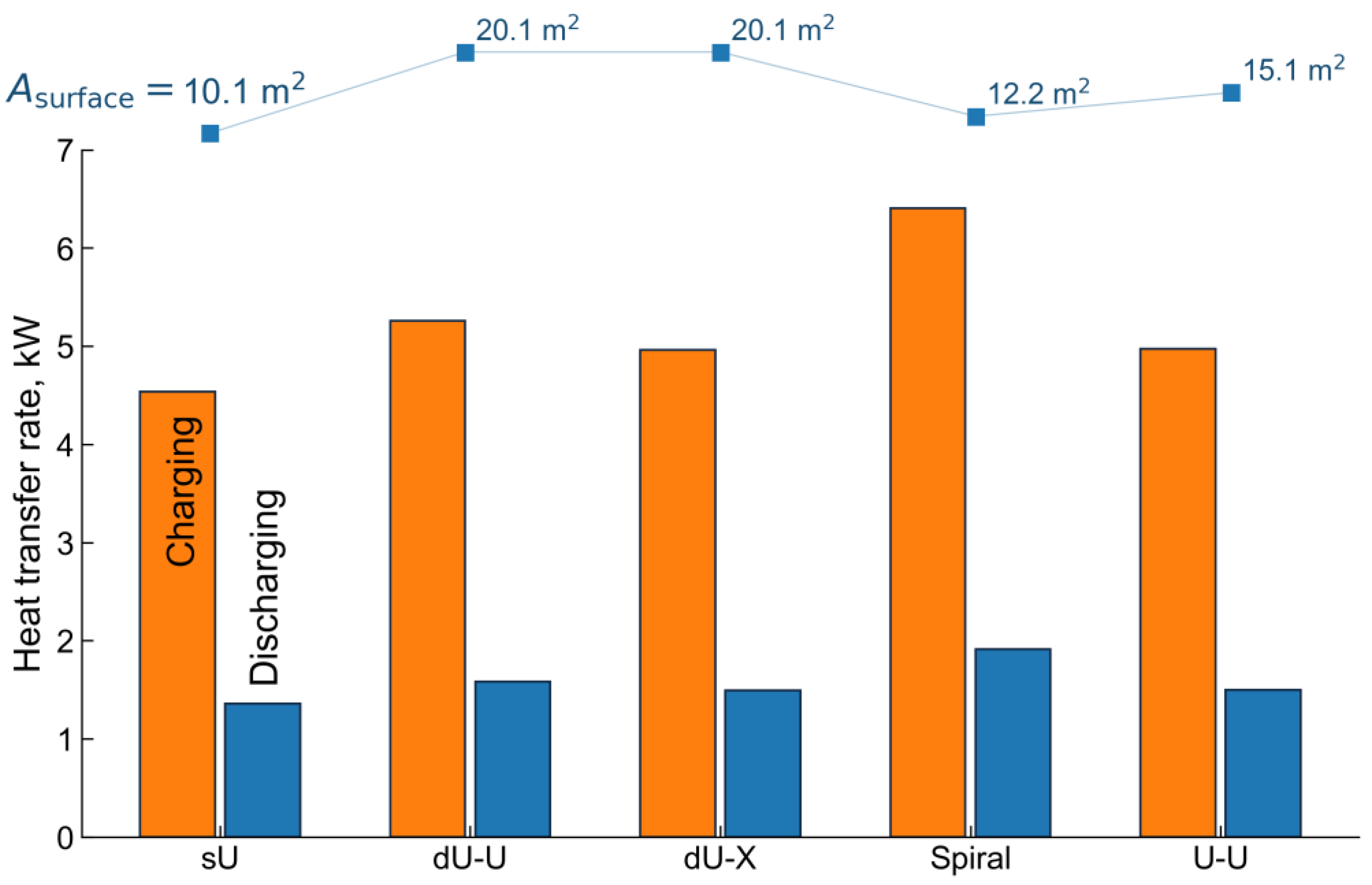
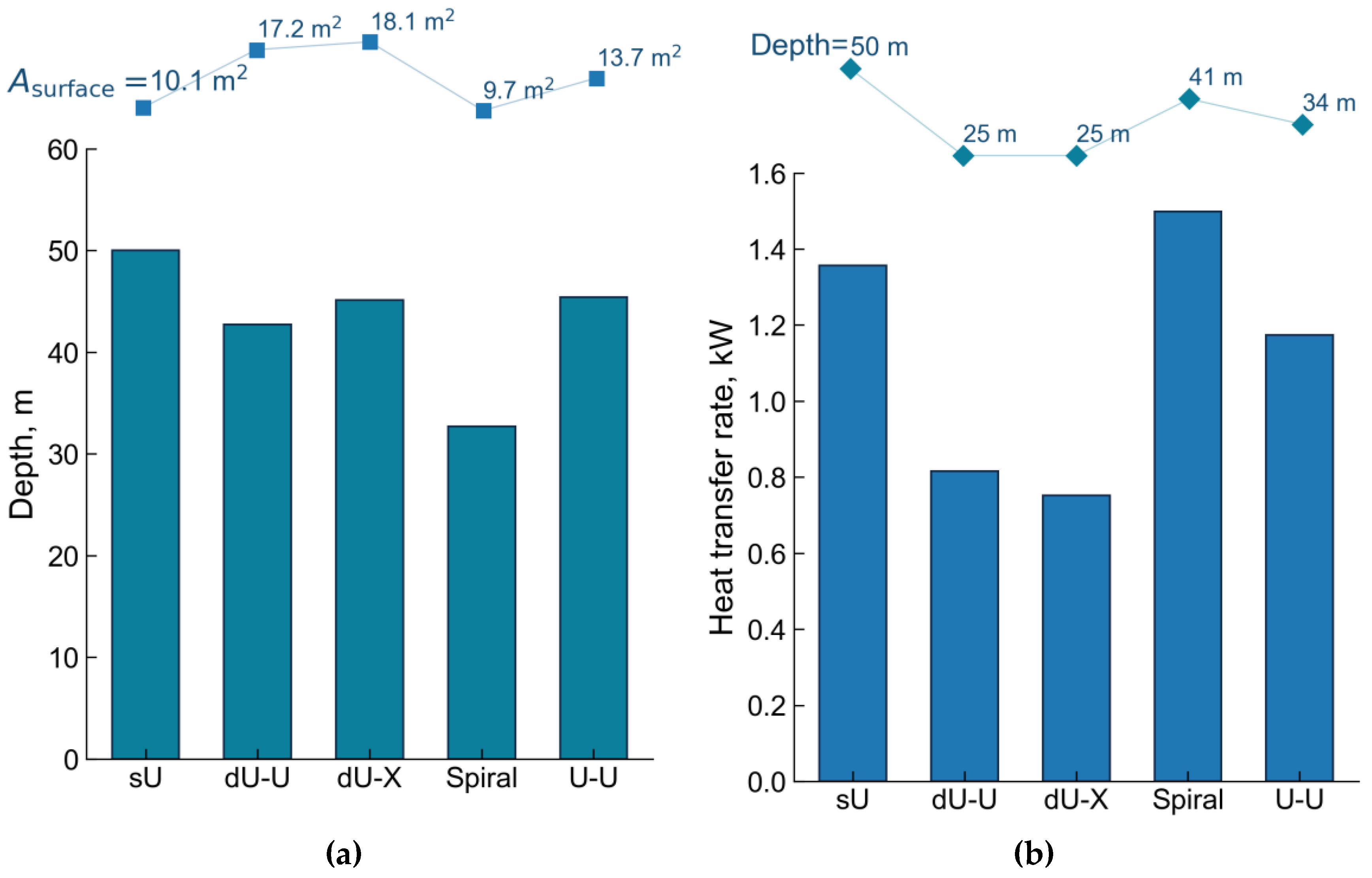
• Based on the numerical results of studying the effect of well depth and heat exchange surface area on heat transfer rates with various geometric configurations, it was found that the spiral configuration demonstrated 34.6% savings at this drilling depth compared to a conventional U-pipe with a value of 0.037 kW/m.
• It is found that the spiral heat exchanger extracts the highest amount of heat, followed by the multi-tube, double U-pipe parallel, double U-pipe cross and single U-pipe.
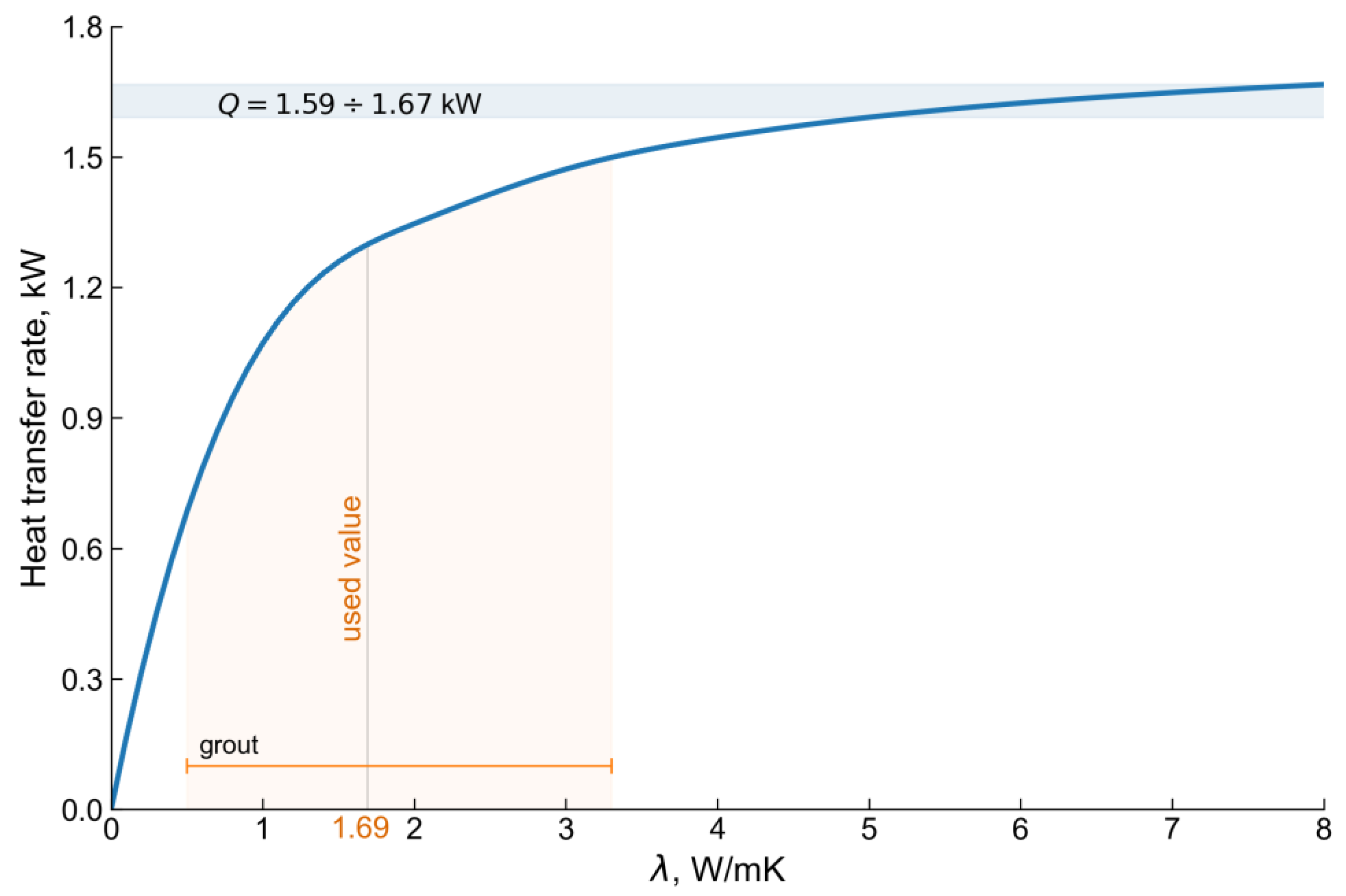
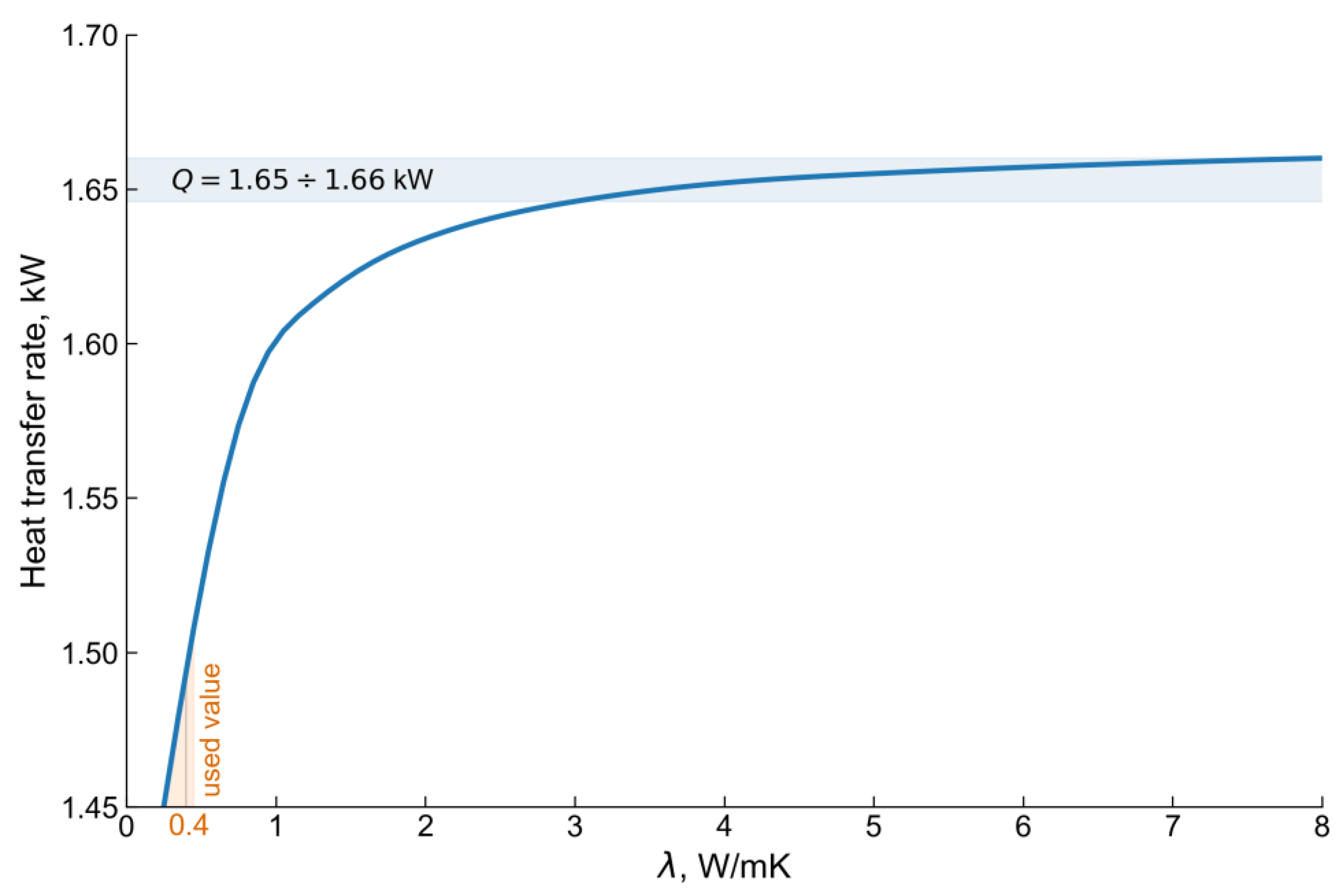
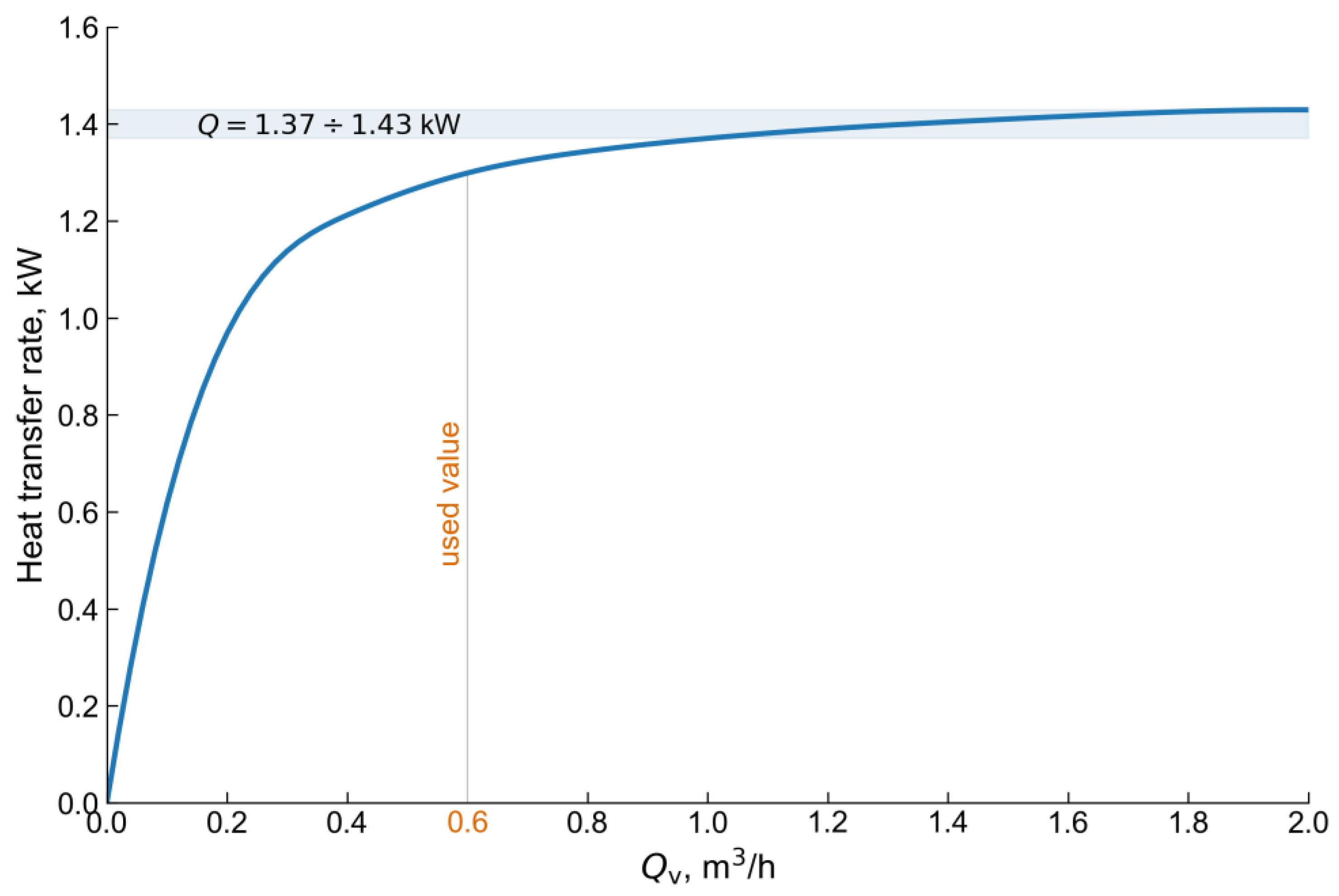
• According to the numerical results of the effect of the thermal conductivity of materials and the circulating fluid flow rate on the heat extraction, it was found that it makes no sense to increase the thermal conductivity of the grout above 3.0 W/m K, the thermal conductivity of the pipe above 2.0 W/m K, and the volumetric flow rate of the circulating fluid above 1.0 m³/h.
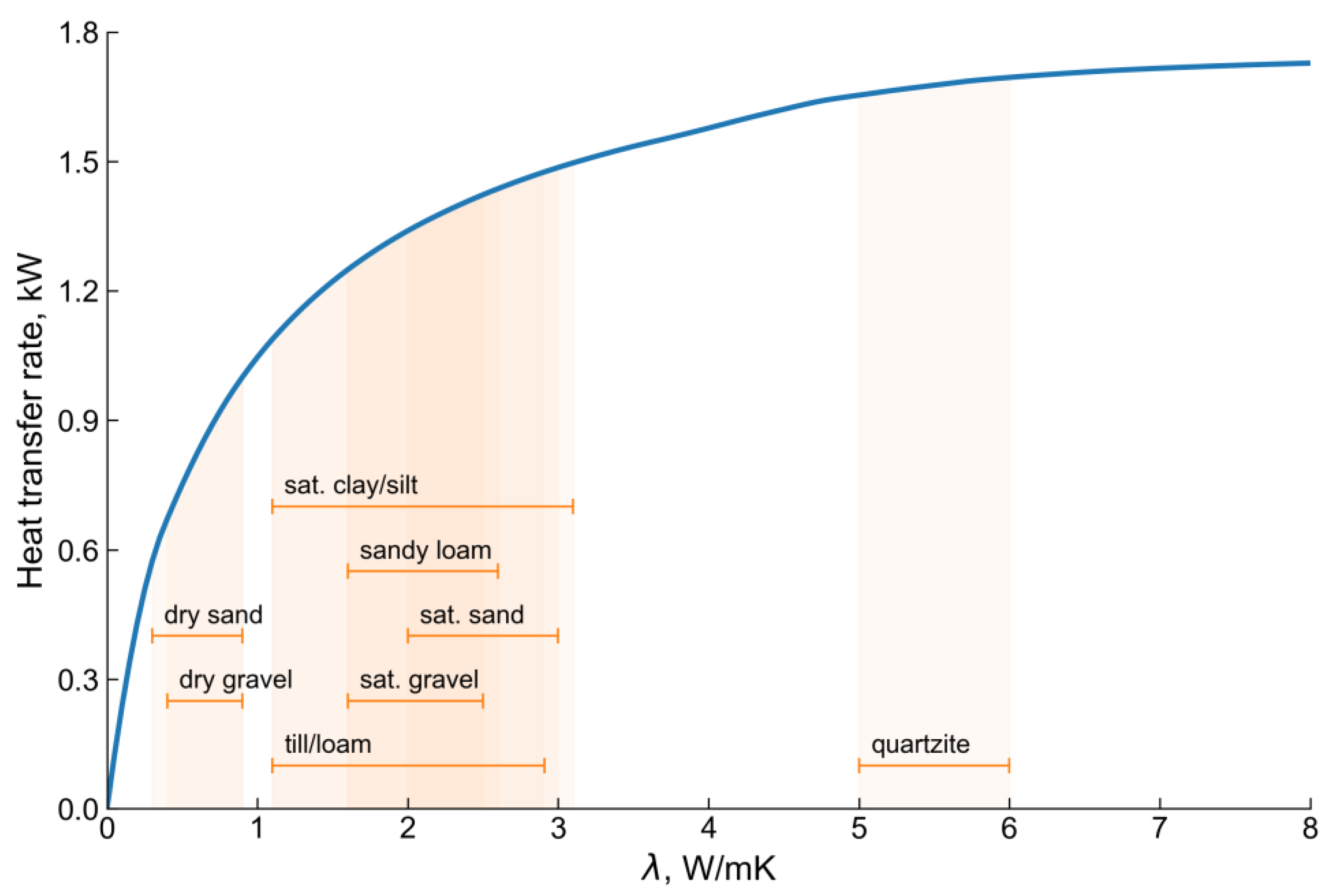
• With an increase in thermal conductivity of the soil, the heat extraction by the borehole heat exchanger increases.
• Regardless of how large the thermal conductivity of the soil is, the heat extraction is limited by the borehole heat exchanger thermal performance.

A prototype ground source heat pump with borehole heat exchangers developed from the present work enables the study of various parameters under different seasonal conditions of the continental climate in Kazakhstan. The model and numerical algorithm developed ensure the prediction of the efficiency of ground heat exchangers, both in relation to heat pumps and to seasonal thermal energy storage. Furthermore, the computational tool developed enables the study of the complex heat and mass transfer in a porous medium and complex geometric configurations of ground heat exchangers.

The scope of future research based on the developed 3D numerical tool includes

• Heat transfer feature modeling around the borehole heat exchanger during charging/discharging modes.
• Heat transfer mechanisms around the borehole heat exchanger, considering the freezing factor during harsh winter conditions.
• Predicting the thermal interference for a system of borehole heat exchangers.
• Multidimensional parametric optimization of borehole heat exchanger thermal performance.

References

1. Johannesson, T.; Axelsson, G.; Hauksdottir, S.; Chatenay, C.; Benediktsson, D.O.; Weisenberger, T.B. Preliminary Review of Geothermal Resources in Kazakhstan; Final Report Rev.2 prepared for the World Bank and the Government of Kazakhstan; World Bank: Washington, DC, USA, 2019; 84p. [Google Scholar]
2. Moya, D.; Aldas, C.; Kaparaju, P. Geothermal energy: Power plant technology and direct heat applications. Renew. Sustain. Energy Rev. 2018, 94, 889–901. [Google Scholar] [CrossRef]
3. Lee, K.C. Classification of geothermal resources–an engineering approach. In Proceedings of the Twenty-First Workshop on Geothermal Reservoir Engineering, Stanford University, Stanford, CA, USA, 22–24 January 1996. [Google Scholar]
4. Muffler, P.; Cataldi, R. Methods for regional assessment of geothermal resources. Geothermics 1978, 7, 53–89. [Google Scholar] [CrossRef] [Green Version]
5. Hochstein, M.P. Classification and assessment of geothermal resources. In Small Geothermal Resources; Dickson, M.H., Fanelli, M., Eds.; UNITAR/UNDP Centre for Small Energy Resources: Rome, Italy, 1990; pp. 31–59. [Google Scholar]
6. Benderitter, Y.; Cormy, G. Possible approach to geothermal research and relative cost estimate. In Small Geothermal Resources; Dickson, M.H., Fanelli, M., Eds.; UNITAR/UNDP Centre for Small Energy Resources: Rome, Italy, 1990; pp. 61–71. [Google Scholar]
7. Haenel, R.; Rybach, L.; Stegena, L. Handbook of Terrestrial Heat-Flow Density Determination; Kluwer Academic: Dordrecht, The Netherlands, 1988; pp. 9–57. [Google Scholar]
8. Cunha, R.P.; Bourne-Webb, P.J. A critical review on the current knowledge of geothermal energy piles to sustainable climatize buildings. Renew. Sustain. Energy Rev. 2022, 158, 112072. [Google Scholar] [CrossRef]
9. Deng, J.; Wei, Q.; He, S.; Liang, M.; Zhang, H. What is the main difference between medium-depth geothermal heat pump systems and conventional shallow-depth geothermal heat pump systems? Field tests and comparative study. Appl. Sci. 2019, 9, 5120. [Google Scholar] [CrossRef] [Green Version]
10. Welsch, B.; Ruhaak, W.; Schulte, D.O.; Bar, K.; Saas, I. Characteristics of medium deep borehole thermal energy storage. Int. J. Energy Res. 2016, 40, 1855–1868. [Google Scholar] [CrossRef]
11. Haehnlein, S.; Beyer, P.; Blum, P. International legal status of the use of shallow geothermal energy. Renew. Sustain. Energy Rev. 2010, 14, 2611–2625. [Google Scholar] [CrossRef]
12. Pratiwi, A.S.; Trutnevyte, E. Life cycle assessment of shallow to medium-depth geothermal heating and cooling networks in the State of Geneva. Geothermics 2021, 90, 101988. [Google Scholar] [CrossRef]
13. Romanov, D.; Leiss, B. Geothermal energy at different depth for district heating and cooling of existing and future building stock. Renew. Sustain. Energy Rev. 2022, 167, 112727. [Google Scholar] [CrossRef]
14. Spitler, J.D.; Gehlin, S.E.A. Thermal response testing for ground source heat pump systems–An historical review. Renew. Sustain. Energy Rev. 2015, 50, 1125–1137. [Google Scholar] [CrossRef]
15. Saktashova, G.; Aliuly, A.; Belyayev, Y.; Mohanraj, M.; Singh, R.M. Numerical heat transfer simulation of solar-geothermal hybrid source heat pump in Kazakhstan climates. Bulg. Chem. Commun. 2018, 50, 7–13. [Google Scholar]
16. Santa, G.D.; Galgaro, A.; Sassi, R.; Cultrera, M.; Scotton, P.; Mueller, J.; Bertermann, D.; Mendrinos, D.; Pasquali, R.; Perego, R.; et al. An updated ground thermal properties database for GSHP applications. Geothermics 2020, 85, 101758. [Google Scholar] [CrossRef]
17. Bertermann, D.; Muller, J.; Freitag, S.; Schwarz, H. Comparison between measured and calculated thermal conductivities within different grain size classes and their related depth ranges. Soil Syst. 2018, 2, 50. [Google Scholar] [CrossRef] [Green Version]
18. Ramos-Escudero, A.; Garsia-Cascales, M.S.; Urchueguia, J.F. Evaluation of the shallow geothermal potential for heating and cooling and its integration in the socioeconomic environment: A case study in the region of Murcia, Spain. Energies 2021, 14, 5740. [Google Scholar] [CrossRef]
19. Reuss, M. The use of borehole thermal energy storage (BTES) systems. In Advances in Thermal Energy Storage Systems, Methods and Applications; Cabeza, F.C., Ed.; Woodhead Publishing: Cambridge, UK, 2015; Volume in Woodhead Publishing Series in Energy; pp. 117–147. [Google Scholar]
20. Gehlin, S. Thermal Response Test: Method, Development and Evaluation. Ph.D. Thesis, Lulea University of Technology, Lulea, Sweden, September 2002. [Google Scholar]
21. Amanzholov, T.; Akhmetov, B.; Georgiev, A.; Kaltayev, A.; Popov, R.; Dzhonova-Atanasova, D.; Tungatarova, M. Numerical modelling as a supplementary tool for thermal response test. Bulg. Chem. Commun. 2016, 48, 109–114. [Google Scholar]
22. Mogensen, P. Fluid to duct wall heat transfer in duct system heat storages. In Proceedings of the International Conference on Subsurface Heat Storage in Theory and Practice, Stockholm, Sweden, 6–8 June 1983; pp. 652–657. [Google Scholar]
23. Luo, J.; Zhang, Y.; Tuo, J.; Xue, W.; Rohn, J.; Baumgartel, S. A novel approach to the analysis of thermal response test (TRT) with interrupted power input. Energies 2020, 13, 5033. [Google Scholar] [CrossRef]
24. Li, P.; Guan, P.; Zheng, J.; Dou, B.; Tian, H.; Duan, X.; Liu, H. Field test and numerical simulation on heat transfer performance of coaxial borehole heat exchanger. Energies 2020, 13, 5471. [Google Scholar] [CrossRef]
25. Piotrowska-Woroniak, J. Determination of the selected wells operational power with borehole heat exchangers operating in real conditions, based on experimental tests. Energies 2021, 14, 2512. [Google Scholar] [CrossRef]
26. Hesselbrandt, M.; Erlstrom, M.; Sopher, D.; Acuna, J. Multidisciplinary approaches for assessing a high temperature borehole thermal energy storage facility at Linkoping, Sweden. Energies 2021, 14, 4379. [Google Scholar] [CrossRef]
27. Giordano, N.; Lamarche, L.; Raymond, J. Evaluation of subsurface heat capacity through oscillatory thermal response tests. Energies 2021, 14, 5791. [Google Scholar] [CrossRef]
28. Morchio, S.; Fossa, M.; Priarone, A.; Boccalatte, A. Reduced scale experimental modelling of distributed thermal response tests for the estimation of the ground thermal conductivity. Energies 2021, 14, 6955. [Google Scholar] [CrossRef]
29. Pambou, C.H.K.; Raymond, J.; Miranda, M.M.; Giordano, N. Estimation of in situ heat capacity and thermal diffusivity from undisturbed ground temperature profile measured in ground heat exchangers. Geosciences 2022, 12, 180. [Google Scholar] [CrossRef]
30. Zhou, A.; Huang, X.; Wang, W.; Jiang, P.; Li, X. Thermo-hydraulic performance of U-tube borehole heat exchanger with different cross-sections. Sustainability 2021, 13, 3255. [Google Scholar] [CrossRef]
31. Wang, C.; Fu, Q.; Fang, H.; Lu, J. Estimation of ground thermal properties of shallow coaxial borehole heat exchanger using an improved parameter estimation method. Sustainability 2022, 14, 7356. [Google Scholar] [CrossRef]
32. Bourhis, P.; Cousin, B.; Loria, A.F.R.; Laloui, L. Machine learning enhancement of thermal response tests for geothermal potential evaluations at site and regional scales. Geothermics 2021, 95, 102132. [Google Scholar] [CrossRef]
33. Li, K.; Liu, Y.; Kang, Q. Estimating the thermal conductivity of soils using six machine learning algorithms. Int. Commun. Heat Mass Transf. 2022, 136, 106139. [Google Scholar] [CrossRef]
34. Kerme, E.D.; Fung, A.S. Heat transfer analysis of single and double U-tube borehole heat exchanger with two independent circuits. J. Energy Storage 2021, 43, 103141. [Google Scholar] [CrossRef]
35. Ingersoll, L.R.; Zobel, O.J.; Ingersoll, A.C. Heat Conduction: With Engineering, Geological, and Other Applications; The University of Wisconsin Press: Madison, WI, USA, 1954; pp. 1–325. [Google Scholar]
36. Zeng, H.Y.; Diao, N.R.; Fang, Z.H. A finite line-source model for boreholes in geothermal heat exchangers. Heat Transf. Asian Res. 2002, 31, 558–567. [Google Scholar] [CrossRef]
37. Hellstrom, G. Duct Ground Heat Storage Model, Manual for Computer Code; Department of Mathematical Physics, University of Lund: Lund, Sweden, 1989. [Google Scholar]
38. Cao, S.J.; Kong, X.R.; Deng, Y.; Zhang, W.; Yang, L.; Ye, Z.P. Investigation on thermal performance of steel heat exchanger for ground source heat pump systems using full-scale experiments and numerical simulations. Appl. Therm. Eng. 2017, 115, 91–98. [Google Scholar] [CrossRef]
39. Rees, S.J.; He, M. A three-dimensional numerical model of borehole heat exchanger heat transfer and fluid flow. Geothermics 2013, 46, 1–13. [Google Scholar] [CrossRef] [Green Version]
40. Bouhacina, B.; Saim, R.; Oztop, H.F. Numerical investigation of a novel tube design for the geothermal borehole heat exchanger. Appl. Therm.Eng. 2015, 79, 153–162. [Google Scholar] [CrossRef]
41. Vella, C.; Borg, S.P.; Micallef, D. The Effect of Shank-Space on the Thermal Performance of Shallow Vertical U-Tube Ground Heat Exchangers. Energies 2020, 13, 602. [Google Scholar] [CrossRef] [Green Version]
42. Akhmetov, B.; Georgiev, A.G.; Kaltayev, A.; Dzhomartov, A.A.; Popov, R.; Tungatarova, M.S. Thermal energy storage systems–review. Bulg. Chem. Commun. 2016, 48, 31–40. [Google Scholar]
43. Akhmetov, B.; Georgiev, A.; Popov, R.; Turtayeva, Z.; Kaltayev, A.; Ding, Y. A novel hybrid approach for in-situ determining the thermal properties of subsurface layers around borehole heat exchanger. Int. J. Heat Mass Transf. 2018, 126, 1138–1149. [Google Scholar] [CrossRef]
44. Luo, J.; Pei, K.; Li, P. Analysis of the thermal performance reduction of a groundwater source heat pump (GWHP) system. Eng. Fail. Anal. 2022, 132, 105922. [Google Scholar] [CrossRef]
45. Boon, D.P.; Farr, G.J.; Abesser, C.; Patton, A.M.; James, D.R.; Schofield, D.I.; Tucker, D.G. Groundwater heat pump feasibility in shallow urban aquifers: Experience from Cardiff, UK. Sci. Total Environ. 2019, 697, 133847. [Google Scholar] [CrossRef]
46. Li, C.; Mao, J.; Peng, X.; Mao, W.; Xing, Z.; Wang, B. Influence of ground surface boundary conditions on horizontal ground source heat pump systems. Appl. Therm. Eng. 2019, 152, 160–168. [Google Scholar] [CrossRef]
47. Liu, X.; He, M.; Wang, Y.; Zheng, B.; Li, C.; Zhu, X. Experimental study on heat transfer attenuation due to thermal deformation of horizontal GHEs. Geothermics 2021, 97, 102241. [Google Scholar] [CrossRef]
48. Sang, J.; Liu, X.; Liang, C.; Feng, G.; Li, Z.; Wu, X.; Song, M. Differences between design expectations and actual operation of ground source heat pumps for green buildings in cold region of northern China. Energy 2022, 252, 124077. [Google Scholar] [CrossRef]
49. Zhang, M.; Liu, X.; Biswas, K.; Warner, J. A three-dimensional numerical investigation of a novel shallow bore ground heat exchanger integrated with phase change material. Appl. Therm. Eng. 2019, 162, 114297. [Google Scholar] [CrossRef]
50. Warner, J.; Liu, X.; Shi, L.; Qu, M.; Zhang, M. A novel shallow bore ground heat exchanger for ground source heat pump applications—Model development and validation. Appl. Therm. Eng. 2020, 164, 114460. [Google Scholar] [CrossRef]
51. Blazquez, C.S.; Martin, A.F.; Nieto, I.M.; Garcia, P.C.; Perez, L.S.S.; Gonzalez-Aguilera, D. Efficiency analysis of the main components of a vertical closed-loop system in a borehole heat exchanger. Energies 2017, 10, 201. [Google Scholar] [CrossRef] [Green Version]
52. Bae, S.M.; Nam, Y.; Choi, J.M.; Lee, K.H.; Choi, J.S. Analysis on thermal performance of ground heat exchanger according to design type based on thermal response test. Energies 2019, 12, 651. [Google Scholar] [CrossRef] [Green Version]
53. Zhang, L.; Shi, Z.; Yuan, T. Study on the coupled heat transfer model based on groundwater advection and axial heat conduction for the double U-tube vertical borehole heat exchanger. Sustainability 2020, 12, 7345. [Google Scholar] [CrossRef]
54. Javadi, H.; Ajarostaghi, S.S.M.; Pourfallah, M.; Zaboli, M. Performance analysis of helical ground heat exchangers with dif-ferent configurations. Appl. Therm. Eng. 2019, 154, 24–36. [Google Scholar] [CrossRef]
55. Zarella, A.; De Carli., M.; Galgaro, A. Thermal performance of two types of energy foundation pile: Helical pipe and triple U-tube. Appl. Therm. Eng. 2013, 61, 301–310. [Google Scholar] [CrossRef]
56. Quaggiotto, D.; Zarella, A.; Emmi, G.; De Carli, M.; Pockele, L.; Vercruysse, J.; Psyk, M.; Righini, D.; Galgaro, A.; Mendrinos, D.; et al. Simulation-Based Comparison Between the Thermal Behavior of Coaxial and Double U-Tube Borehole Heat Ex-changers. Energies 2019, 12, 2321. [Google Scholar] [CrossRef] [Green Version]
57. Feidt, M. Finite Physical Dimensions Optimal Thermodynamics 1; Elsevier ISTE Press Ltd.: Amsterdam, The Netherlands, 2017; p. 245. [Google Scholar] [CrossRef]
58. Feidt, M. Finite Physical Dimensions Optimal Thermodynamics 2; Elsevier ISTE Press Ltd.: Amsterdam, The Netherlands, 2018; p. 194. [Google Scholar] [CrossRef]
59. Colombo, L.P.M.; Lucchini, A.; Molinaroli, L. Experimental analysis of the use of R1234yf and R1234ze(E) as drop-in alternatives of R134a in a water-to-water heat pump. Int. J. Refrig. 2020, 115, 18–27. [Google Scholar] [CrossRef] [Green Version]
60. Molinaroli, L.; Lucchini, A.; Colombo, L.P.M. Drop-in analysis of R450A and R513A as low-GWP alternatives to R134a in a water-to-water heat pump. Int. J. Refrig. 2022, 135, 139–147. [Google Scholar] [CrossRef]
61. Yerdesh, Y.; Amanzholov, T.; Aliuly, A.; Seitov, A.; Toleukhanov, A.; Murugesan, M.; Botella, O.; Feidt, M.; Wang, H.S.; Tsoy, A.; et al. Experimental and Theoretical Investigations of a Ground Source Heat Pump System for Water and Space Heating Applications in Kazakhstan. Energies 2022, 15, 8336. [Google Scholar] [CrossRef]
62. Russian Geological Research Institute (VSEGEI). Available online: https://rasterdb.vsegei.ru/img.php?id=41510 (accessed on 29 September 2022).
63. Erol, S.; Grathwohl, P.; Blum, P.; Bayer, P. Estimation of Heat Extraction Rates of GSHP Systems under Different Hydrogeological Conditions. Ph.D. Thesis, University of Tuebingen, Tübingen, Germany, 2011. [Google Scholar]
64. Carslaw, H.S.; Jaeger, J.C. Conduction of Heat in Solids; Oxford University Press: Oxford, UK, 1959; pp. 1–310. [Google Scholar]
65. Gnielinski, V. New Equations for Heat and Mass Transfer in Turbulent Pipe and Channel Flow. Int. Chem. Eng. 1976, 16, 359–368. [Google Scholar]
66. Churchill, S.W. Friction factor equation spans all fluid-flow regimes. Chem. Eng. 1997, 84, 91–92. [Google Scholar]
67. Allan, M.L.; Kavanaugh, S.P. Thermal conductivity of cementitious grouts and impact on heat exchanger length design for ground source heat pumps. HVACR Res. 1999, 5, 85–96. [Google Scholar] [CrossRef]
Figure 1. Thermal Response Test at Koksai mosque, Almaty.
Energies 15 08490 g001
Figure 2. Geological structure defined during the drilling.
Energies 15 08490 g002
Figure 3. Computational domains for the borehole heat exchanger.
Energies 15 08490 g003
Figure 4. Temperature variation at the inlet and outlet parts of the BHE.
Energies 15 08490 g004
Figure 5. Undisturbed initial temperature of the ground with depth.
Energies 15 08490 g005
Figure 6. Undisturbed reference temperature of the ground.
Energies 15 08490 g006
Figure 7. Energy performance of the BHE.
Energies 15 08490 g007
Figure 8. Regression line for temperature vs. time (full time, 7 days).
Energies 15 08490 g008
Figure 9. Regression line with different time intervals, excluding the first 10 h, 24 h, and 48 h.
Energies 15 08490 g009
Figure 10. Comparison of the numerical and experimental data for T o u t of HTF in BHE.
Energies 15 08490 g010
Figure 11. Grid sensitivity analysis.
Energies 15 08490 g011
Figure 12. Geometric configurations of BHE.
Energies 15 08490 g012
Figure 13. Heat transfer rates for various pipe configurations at a 50 m well depth.
Energies 15 08490 g013
Figure 14. Geometric parameter effects: (a) well depths for various pipe configurations at a constant heat flow Q = 1350 W; (b) heat transfer rates for various pipe configurations with a constant heat exchange surface area A s u r f a c e = 10.05 m2.
Energies 15 08490 g014
Figure 15. Dependence of the heat transfer rate on the grout thermal conductivity.
Energies 15 08490 g015
Figure 16. Dependence of the heat transfer rate on the pipe material thermal conductivity.
Energies 15 08490 g016
Figure 17. Dependence of the heat transfer rate on the HTF volumetric flow rate.
Energies 15 08490 g017
Figure 18. Dependence of the heat transfer rate on the soil thermal conductivity.
Energies 15 08490 g018