Article

Optimization of Cogeneration Power-Desalination Plants

by
Ariana M. Pietrasanta
1,
Sergio F. Mussati
1,
Pio A. Aguirre
1,
Tatiana Morosuk
2,* and
Miguel C. Mussati
1
1
INGAR Instituto de Desarrollo y Diseño (CONICET-UTN), Avellaneda 3657, Santa Fe 3000, Argentina
2
Institute for Energy Engineering, Technishe Universität Berlin, Marchstrs. 18, 10623 Berlin, Germany
*
Author to whom correspondence should be addressed.
Energies 2022, 15(22), 8374; https://doi.org/10.3390/en15228374
Submission received: 19 September 2022 / Revised: 24 October 2022 / Accepted: 25 October 2022 / Published: 9 November 2022
(This article belongs to the Special Issue Exergoeconomic Analysis of Thermal Systems)

Abstract

:
The design of new dual-purpose thermal desalination plants is a combinatory problem because the optimal process configuration strongly depends on the desired targets of electricity and freshwater. This paper proposes a mathematical model for selecting the optimal structure, the operating conditions, and sizes of all system components of dual-purpose thermal desalination plants. Electricity is supposed to be generated by a combined-cycle heat and power plant (CCHPP) with the following candidate structures: (a) one or two gas turbines; (b) one or two additional burners in the heat recovery steam generator; (c) the presence or missing a medium-pressure steam turbine; (d) steam generation and reheating at low pressure. Freshwater is supposed to be obtained from two candidate thermal processes: and (e) a multi-effect distillation (MED) or a multi-stage flash (MSF) system. The number of effects in MED and stages in MSF are also discrete decisions. Different case studies are presented to show the applicability of the model for same cost data. The proposed model is a powerful tool in optimizing new plants (or plants under modernization) and/or improving existing plants for desired electricity generation and freshwater production. No articles addressing the optimization involving the discrete decisions mentioned above are found in the literature.

1. Introduction

Seawater desalination represents a pivotal technology to meet the freshwater supply required for rapid population growth. More than twenty thousand desalination plants are currently under operation in 150 countries. The majority of the large-scale seawater desalination plants are dual-purpose ones. For power generation, either steam or combined-cycle heat and power plants (CCHPP) are used. The steam is extracted at a temperature that is required by a thermal seawater desalination plant. Dual-purpose power desalination plants (DPPDP) offer several benefits over stand-alone desalination plants: significant reductions in costs and increases in overall energy efficiencies. The electricity and freshwater demands are the major design specifications, which can be met with several process structures and designs, leading to a combinatory problem. The power-to-water cogeneration plant (El-Nashar [1]). Then, optimizing the process schemes (configurations) and operating conditions play an important role in proposing cost-effective designs of DPPDPs.
The study on DPPDPs was carried out considering:
  • different types of power generation plants and desalination systems—Shahzad et al. [2], Eveloy et al. [3], Mokhtari et al. [4], Al-Zahrani et al. [5], Ansari et al. [6], Wu [7], Tian et al. [8], Eltamaly et al., 2021 [9], Ali et al., 2021 [10], and
  • several computational tools—ASPEN (Luo et al. [11]), EES (Tamburini et al. [12]), MATLAB and Termoflex (Modabber and Manesh [13]), GAMS (Manassaldi et al. [14], and Mussati et al. [15]).
Shahzad et al. [2] studied a CCHPP and multi-effect distillation (MED) desalination system by applying an exergy-based analysis to develop an improved fuel cost estimation method. The authors found that the exergy destruction of the desalination unit is about 2–7% of the total exergy destruction. Eveloy et al. [3] investigated the integration of a pressurized solid oxide fuel cell–gas turbine (SOFC-GT) hybrid system and a reverse osmosis (RO) plant. With the help of a genetic algorithm (GA), they conducted the multi-objective optimization using exergetic efficiency and total cost as objective functions. They coupled the ASPEN process simulation with a non-dominated sorting multi-objective GA supported by MATLAB. The different working fluids for the organic Rankine cycle (ORC) were considered. Mokhtari et al. [4] and Al-Zahrani et al. [5] studied integrated systems consisting of a GT system and MED and RO desalination processes. Al-Zahrani et al. [5] implemented a mathematical model of the entire process using Engineering Equations Solver (EES) to evaluate the values of the exergy destruction in the process components. The GT combustion chamber showed the highest irreversibility, followed by the HRSG. The MED process with thermal vapor compression (TVC) contributed 18% to the total exergy destruction. Several authors investigated the integration of the pressurized water reactor (PWR) in nuclear power plants and desalination systems (Ansari et al. [6], Wu [7], and Tian et al. [8]). Ansari et al. [6] conducted the optimization using GA. Three optimization problems were considered: a single-objective thermodynamic, a single-objective thermoeconomic, and a multi-objective. In the multi-objective optimization (MOO), the minimization of the product costs (electricity and freshwater) and the maximization of the overall exergetic efficiency were solved using the Pareto frontier. In the thermoeconomic optimization, the cost of generated power and freshwater production was reduced by 13.4% and 27.5%, respectively, with respect to a selected base case. Eltamaly et al. [9] and Ali et al. [10] investigated hybrid renewable energy systems combining solar and wind energies with reverse osmosis desalination units. Eltamaly et al. [9] applied different optimization approaches, such as particle swarm optimization (PSO), bat algorithm (BA), and others, based in social mimic technique. Optimization results show the preference of usage BA algorithms compared to the other ones.
By using ASPEN Plus, Luo et al. [11] investigated a DPPDP consisting of a chemically recuperated gas turbine (CRGT) and a MED-TVC system. They proposed to replace the superheater of the HRSG by a steam methane reformer (SMR) to produce syngas. The property estimation packages supported in ASPEN ‘RK-SOAVE’, ‘STEAM-TA’, and ‘ELECNRTL’ were used to calculate the properties of the working gas fluid, water, and seawater, respectively. The authors found that the proposed CRGT system is economically attractive only if a low-cost source of water is available. Using EES, Tamburini et al. [12] studied the retrofitting of existing CHP systems considering a MED process with TVC technology. They developed an analytical model to simulate plant operation under different operating conditions.
In addition, some publications addressing different optimization methods should be mentioned: metaheuristic approaches (Wu et al. [16], Shakib et al. [17], Hosseini et al. [18], Modabber and Manesh [19]) and deterministic approaches (Zak [20], Manassaldi et al. [14], Mussati et al. [15]. Wu et al. [16] proposed a mixed-coded GA to solve a mixed-integer nonlinear programming (MINLP) model to optimize the process configuration and operation conditions to satisfy specified electricity and freshwater demands at a minimum total annual cost (TAC). They proposed a boiler and two candidate steam turbines for the power plant—a back-pressure turbine and an extraction–condensation turbine—which are modeled as discrete decisions. They proposed modifications to the classic GA to consider these discrete decisions. For seawater desalination, a hybrid MSF/RO system is considered. The resulting model and solution strategy were applied to several case studies considering different freshwater demand levels. Shakib et al. [17] investigated a DPPDP consisting of a GT with and without an air preheater (APH), HRSG, and MED-TVC. After simulating the process and performing a thermoeconomic analysis, a multi-objective genetic algorithm (MOGA) is applied to achieve the optimal design at the minimum cost of products and maximal exergy efficiency. Zak [20] highlighted the need for numerical optimization and detailed modeling to obtain cost-effective DPPDPs. One of the main advantages of metaheuristic-based optimization approaches is that there is no need for the analytical knowledge of the equations system (i.e., gradient information of the design variables, including the objective function), and there is a requirement for low computational resources in providing solutions. However, they are derivative-free approaches at the same time, which is a disadvantage from a rigorous optimization point of view, because the optimality of the solutions cannot be guaranteed. Then, deterministic and gradient-based optimization approaches are preferred over metaheuristic approaches. Manassaldi et al. [14] recently developed a deterministic MINLP technique to address the optimal revamping of an existing DPPDP. Several optimization scenarios were investigated by using the simple branch and bound (SBB) [21] as the derivative-based MINLP solver. One of them consisted in optimizing the HRSG of the integrated CCHP/MSF desalter system by keeping the same size of the GT and the same configuration of the MSF desalter as in the existing plant. The influence of three-pressure (3P), two-pressure (2P), and one-pressure (1P) heat recovery steam generators (3P-, 2P-, and 1P-HRSG, respectively) on the overall energy efficiency was investigated.
The novelty of this work is to develop a deterministic mathematical model of combined power and desalination systems that allows a systematic optimization of the configuration, the sizes of the process components, and operating conditions to meet desired electricity and freshwater demand at a minimum total annual cost. In this work, the number of candidate configurations is much higher than those considered in [14,15,20]. For instance, besides considering several candidate configurations involved in the CCHP, two thermal desalting processes (MED and MSF) are the candidates to produce freshwater, significantly increasing the combinatory nature of the problem and the degrees of freedom—the associated trade-offs between the variables—for optimization. In addition, this work differs from [20] in the application of a deterministic optimization approach instead of a metaheuristic algorithm.

2. Process Description

Figure 1 shows a general configuration of a DPPDP consisting of a CCHP and a MED desalination process.
The CCHP consists of a compressor (COMP), a combustion chamber (CC), and a gas turbine (GT). The exhaust gases are used for the 2P-HRSG to produce steam. A part of the steam leaving the steam turbine ST1 (S) is forwarded to the thermal desalination (multi-effect distillation or multi-stage flash desalination units) to be used as the heating source. The main design specification of any DPPDP is the ratio of the required electricity to freshwater production (PWR), which strongly influences the optimal structure and operating conditions. Typical PWR values expressed in MW power generated per million gallons per day of water produced range from 3 to 20.
The simplest configuration of a combined-cycle power and desalination plant involves a back-pressure steam turbine with a one-pressure heat recovery steam generator (1P-HRSG). The HRSG can be designed for one, two, or three pressure levels influencing the steam turbine network. For high PWR values, the power plant design is more critical than the design of the desalination plant. For instance, for PWR values higher than 8, the structure of the HRSG could involve two or three pressure levels with reheating of steam at medium (or low) pressure level and/or auxiliary boilers. For low PWR values, the design of the desalination process is more critical than the design of the power plant. For instance, for PWR values lower than 3, the freshwater demand could be satisfied with a large MED unit or a medium-small MSF unit involving a simple HRSG, i.e., one pressure or two pressure levels. For values of PWR between 3 and 8, the designs of the power and desalination plants have the same importance.
In Figure 1, the CCHPP was coupled with a MED desalination system, which can be replaced with a MSF system, obtaining other configurations of DPPDPs.

2.1. Multiple Stage Flash (MSF) Desalination System

Figure 2a illustrates a simplified schematic of a MSF desalination system, and Figure 2b shows the representative system for the mathematical modeling.
The MSF system involves several stages. Each stage includes a preheater (HEX), primary flashing chambers (PFC, brine flashing), secondary flashing chambers (SFC, distillate flashing), and the main brine heater (MBH). In the HEXs, the incoming seawater stream F is heated from TSW to T1F to reach the maximum allowable temperature (Tmax) in the MBH by using steam extracted from the CCHP cycle. The heated seawater F enters the flashing chamber of the first stage PFC1, where a flash boiling of a stream is carried out. The vapor formed in the first stage PFC1 condenses in the associated pre-heater HEX1, pre-heating the incoming seawater F. The distillate leaving the HEX1 (freshwater) is collected in the corresponding distillate plate of stage SFC1 and is passed to the next stage flowing in parallel with the brine stream B1. The brine leaving the first stage (B1) enters the second stage PFC2 and the vapors formed are mixed with the vapor formed by the distillate stream SFC2, and the resulting vapor stream is used as a heating source in the HEX2. The boiling/condensation process of the brine and distillate streams is repeated until the last stage. The concentration profile increases from the first to the last stage. To reduce the incoming seawater SW and the associated pretreatment cost, a part of the brine leaving the last stage is often recycled by mixing it with the incoming seawater. A desalination plant operating in this mode is often referred to as a “brine recycle” plant.

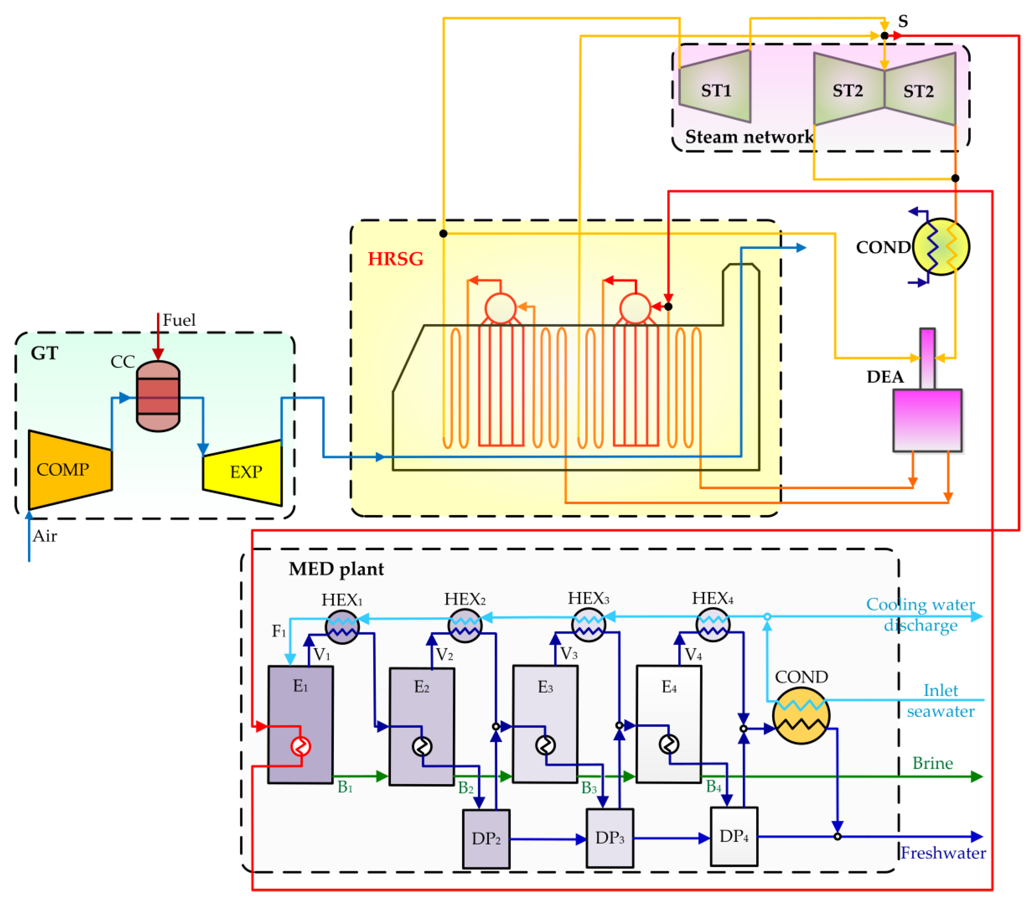
2.2. Multi-Effect Distillation (MED) Desalination System

Figure 3a illustrates a simplified schematic of a MED desalination system, and Figure 3b shows the representative system for mathematical modeling. Despite the working principle of the MED system involving evaporation of brine and condensation of vapor as in the MSF system, the evaporation/condensation processes and the heat transfer mechanism are different. In the MED units, the evaporation process is carried out from a seawater film in contact with a heat transfer area, while in the MSF units, the evaporation is carried out from a flow of brine flashing due to the pressure drop applied to each stage without using a heat exchanger. Thus, the brine B is sprayed as a thin film on the tube’s external surface, and the steam formed in the previous effect V flows inside the tube providing the energy required by the evaporation process.
Additionally, compared to the MSF process, the MED process operates at lower temperatures (70–90 °C), which is beneficial for reducing tube corrosion and scale formation on the tube surfaces. In addition, the MED technology might be preferred over the MSF technology for lower freshwater production rates because it could involve lower total costs. For higher production rates, the MSF technology could be preferred over the MED technology because of its lower risk and consolidation in the market. Thus, the selection of the desalination system depends on the design specifications (freshwater production in a single desalination plant and freshwater production and electricity generation in a dual-purpose desalination plant).

3. Problem Statement

Figure 4 shows the superstructure DPPDPs that are used for structure optimization. In the proposed superstructure, several candidate configurations are simultaneously embedded for optimization. For instance, regarding the gas turbine cycle, the superstructure in Figure 4 includes two candidate gas turbines (GT1–39.1 MW and GT2–64.3/67.5 MW), but only one gas turbine must be selected. As it will be presented later, the selection of the gas turbine involves a discrete decision, precisely, a binary variable that is associated to the gas turbine in the node N1. These gas turbines differ in the power capacity, pressure ratio, fuel consumption, and conditions of the exhaust gases (pressure, temperature, and flow rate). Regarding the HRSG, the following candidate options are considered: (a) burner BURN1 and/or BURN2, (b) steam reheating at the medium-pressure level through the splitter SP1 (indicated in blue color in Figure 4), and (c) steam generation and reheating at low-pressure (indicated in green color). Finally, regarding seawater desalination, fresh water can be produced by a MED or MSF system. The selection of the desalination unit is carried out in the splitter SP_DES through a binary variable, as it will be described in the following section. Combining all the mentioned options leads to a total number of feasible process combinations higher than 50. The higher the number of combinations, the higher the chances of finding cost-effective designs are. In the Section 4, the constraints used to model each one of the discrete decisions embedded in Figure 4 are presented.
The optimization problem is stated as follows:
Min TAC (annCAPEX + OPEX)
Subject to:
  • mass balances;
  • energy balances;
  • design equations;
  • cost model;
  • process conditions (seawater temperature and salinity);
  • design specifications (desired levels of electricity and freshwater production).
By solving the proposed model, the following results are simultaneously obtained:
  • the minimum total annual cost (TAC);
  • optimal distribution among annCAPEX and OPEX;
  • optimal selection of the configuration of the entire process (electricity generation plant + desalination process);
  • optimal sizes of all process components selected;
  • optimal operating conditions of all process streams.

4. Modeling Assumptions and Mathematical Model

The main assumptions considered as a first approximation for modeling the MSF and MED desalination systems and the CCHPP are presented below.

4.1. Thermal Desalination Systems

The following assumptions were used for the simulation of the thermal desalination systems:
  • The number of distillation effects in the MED and number of stages in the MSF are treated as continuous variables.
  • Average salinity and temperature values of the brine at operating conditions are considered for estimating the boiling point elevation.
  • The heat load and heat transfer area of the pre-heaters in the MSF process are considered as optimization variables (Al-Mutaz and Wazeer [22]).
  • The same optimization variable is considered for the heat loads and heat transfer areas along the pre-heaters in the MSF process are assumed (Al-Mutaz and Wazeer [22]).
  • The heat load and heat transfer area of the evaporation effects in the MED process are considered as optimization variables (Al-Mutaz and Wazeer [22]).
  • The same optimization variable is considered for the heat loads and heat transfer areas along the evaporation effects in the MED process are assumed (Al-Mutaz and Wazeer [22]).
  • Vapor streams leaving the MED effects and MSF stages are salt-free (El-Dessouky and Ettouney [23], Al-Mutaz and Wazeer [22]).
  • An effective driving force for the heat transfer in the evaporation effect/stage represents an optimization variable (Al-Mutaz and Wazeer [22]).
  • The same optimization variable is associated with the effective driving forces for the heat transfers along all effects/stages (Al-Mutaz and Wazeer [22]).
  • The evaporation effects/stages are optimized under adiabatic conditions (El-Dessouky and Ettouney [23]; Al-Mutaz and Wazeer [22]).

4.2. Combined Cycle Heat and Power Plant

The following assumptions were used for the simulation of the combined cycle heat and power plants:
  • Steady-state condition is considered.
  • A fixed and known value of pressure drop in the HRSG is assumed.
  • Pinch-point temperature differences in all heat exchangers (economizers, evaporators, superheaters, and condensers) are optimization variables with imposed lower bounds [14].
  • Complete combustion with excess air is assumed. CO2, H2O, O2, and N2 are present in the combustion gas.
  • Fixed overall heat transfer coefficients are assumed [14].
  • Heat transfer areas are estimated using the approximation from [24] to overcome numerical difficulties arising from the logarithm mean temperature difference (LMTD) computation.
  • Dependence of the ideal gas thermodynamic properties of the combustion gases with temperature is considered [14].
The DPPDP mathematical model was developed taking into consideration the assumptions listed above and the nomenclature included in Figure 2b, Figure 3b and Figure 4. A set of equations describing the MSF and MED processes and the CCHPP are included in the Appendix A. Here, the main constraints used to model the discrete decisions associated with the candidate structures embedded in Figure 4 is presented.

4.3. Selecting the Optimal Gas Turbine (GT1 or GT2)

As mentioned, a gas turbine must be selected from two options: GT1–39.1 MW or GT2–64.3/67.5 MW. Then, an optimization binary variable yGT1 associated to GT1 in the node N1 is defined and used in Equations (1)–(5) to calculate the values of P2, Air, Fuel, ηAC, and ηGT in terms of parameter values characterizing GT1 and GT2:
P 2 = R P G T 1 y G T 1 + R P G T 2 ( 1 y G T 1 ) P 1  
m A i r = m A i r , G T 1 y G T 1 + m A i r , G T 2 ( 1 y G T 1 )  
m F u e l = m F u e l , G T 1 y G T 1 + m F u e l , G T 2 ( 1 y G T 1 )  
η A C = η A C , G T 1 y G T 1 + η A C , G T 2 ( 1 y G T 1 )  
η E X P = η E X P , G T 1 y G T 1 + η E X P , G T 2 ( 1 y G T 1 ) .
If yGT1 = 1, then GT1 is selected and, according to Equations (1)–(5), the values of P2, mAir, mFuel, ηAC, and ηGT are calculated with the parameter values corresponding to GT1 (P2 = RPGT1·P1, Air = ṁAir,GT1, Fuel = ṁFuel,GT1, ηAC = ηAC,GT1, and ηGT = ηGT1); otherwise, with the parameter values corresponding to GT2. Then, with these values, the corresponding electrical power required by the air compressor and the power generated by the expander are calculated.
It is important to note that, as the gas turbine can be selected from two options, only one binary variable is needed. If more than two gas turbine types are candidates, then Equations (1)–(5) are no longer valid, and the definition of a binary variable for each gas turbine type yGT is needed. For this case, the Equations (1)–(5) should be replaced by Equations (1a)–(5a):
P 2 = G T = G T 1 n R P G T P 1 y G T  
m · A i r = G T = G T 1 n m · A i r , G T y G T  
m · F u e l = G T = G T 1 n m · F u e l , G T y G T  
η A C = G T = G T 1 n η G T y G T  
η E X P = G T = G T 1 n η E X P y G T
It should be mentioned that the complete set of equations describing the gas turbine is included in the model in order to have the possibility to optimize the size and operating conditions for new designs, i.e., without using data taken from manufacturer catalogues. In this work, only two candidate gas turbines are proposed in order to see how well the entire model works from the convergence point of view. In future works, the model will be extended to include more gas turbine candidates by considering Siemens F-Class and H-Class types taken from the literature [25].

4.4. Selection/Removal of Additional Burners and Steam Generation and Reheating at Low-Pressure Level

The selection/removal of the burners BURN1 and BURN2 and the steam generation and reheating at the low-pressure level, indicated in green color in Figure 4, does not require the use of binary variables because they can be selected directly from the mass and energy balances of the process units associated to them. For instance, consider the mass and energy balances around the burner BURN1, which are expressed in Equations (6) and (7):
m · 7 = m · 5 + m · 6  
m · 7 h 7 = m · 5 h 5 + m · 6 h 7 .
If the optimal value for the fuel mass flow rate m · 6 is zero, then the burner BURN1 is removed, and according to the mass and energy balances in Equations (6) and (7): m · 5 = m · 7 and h5 = h7. Otherwise, it is selected by the optimization algorithm.
Equations (8) and (9) are proposed for the selection of the burner BURN2, similarly to that proposed for BURN1:
m · 12 + m · 7 = m · 13  
m · 12 h 12 + m · 7 h 8 = m · 13 h 13 .
Then, if m · 12 = 0, then the burner BURN1 is removed, and according to the mass and energy balances in Equations (8) and (9): m · 7 = m · 13 and h8 = h13. Otherwise, BURN2 is selected by the optimization algorithm.
On the other hand, Equations (10)–(12) are proposed for the selection of the steam generation at the low-pressure level:
m · 10 = m · 11 + m · 11 a  
m · 11 M U P y R E C  
m · 11 M L O y R E C .
If the optimal value is yREC = 0, then, according to constraints Equation (11) and (12) m · 11 = 0 ( m · 10 =  m · 11 a ), indicating that no steam reheating is selected; otherwise, the reheating is included and the optimization variable m11 is bounded between MLO and MUP.

4.5. Selection of the Optimal Desalination System: MED System or MSF System

In a similar way, a binary variable yMSF is defined and associated with the steam required by the MSF desalination unit. Then, the following constraints are derived from the splitter SP_DES (Figure 4):
m · 42 , M S F M U P y M S F  
m · 42 , M S F M L O y M S F  
m · 42 , M E D M U P ( 1 y M S F )  
m · 42 , M E D M L O ( 1 y M S F ) .
If the optimal value is yMSF = 0, then, according to constraints Equations (13) and (14), ṁ42_MSF = 0, indicating that no steam is supplied to the MSF unit and, therefore, it is removed from the optimal solution. At the same time, according to constraints Equations (15) and (16), 42_MED > 0, thus assuring that steam is supplied to the MED unit.

5. Model Implementation Aspects

The resulting MINLP model for the superstructure-based representation was implemented in general algebraic modeling system (GAMS), which is a high-level modeling system for mathematical programming and optimization. It deals with algebraic equations that are solved simultaneously. Discrete and continuous optimizer (DICOPT) code was used as the MINLP solver. By employing an iterative process, it solves a series of nonlinear programming (NLP) and mixed-integer linear (MIP) sub-problems. The optimization algorithm stops when the difference in the solutions obtained from these two problems is less than a pre-defined tolerance.

6. Results

Once the model was implemented and successfully verified, it was used to solve the optimization problem stated in Section 3 by using the parameter values listed in Table 1 and Table 2.
Figure 5 shows the optimal solution obtained by minimizing the TAC. A minimum TAC value of 45.944 MM USD/y (5743.2 USD/h) was obtained, where the CCHPP represents around 85%. As shown in Figure 5, the optimization algorithm selected from the proposed superstructure is the gas turbine GT1–39.1 MW, the first burner BURN1, steam reheating at the medium-pressure level RH1, and the MSF desalination process. The gas turbine GT2–64.3/67.5 MW, the second burner BURN2, steam reheating at the low-pressure level EVP2/SH2, and the MED desalination unit were removed. Regarding the electrical power generation, the steam turbine STs generate 41.91 MW, of which 6.92 MW are generated in HPST, 25.34 MW in MPST, and 9.65 MW in LPST, while the remaining electrical power is generated in the selected gas turbine GT1 (39.1 MW). The optimal pressure value for the HP level is 131.0 bar and 60.0 bar for the MP level. In the MPST, the steam expands from 60.0 bar to 3.29 bar.
The total heat load recovered by the HRSG is 393.6 MW, with the following distribution among its components: 43.9 MW in two superheaters, 41.9 MW in the evaporator, and 40.1 MW in two economizers. This total heat load requires 26,787 m2 of heat transfer area.
Regarding the desalination process, the selected MSF system requires 42 MW as a heating source, which is extracted from the CCHPP before passing through LPST, at a flow rate of 18.55 kg/s. The total heat transfer area required by the MSF is 64,093 m2, which is distributed in 24 flashing stages.
Several optimization problems were solved for the same design specifications, process data, and cost model with the aim of obtaining suboptimal solutions for investigating how much better the optimal configuration presented above is with respect to other configurations. To achieve it, different process configurations were fixed by properly setting the values of the discrete decisions. The main results are compared in Table 3. Figure 6 illustrates a sub-optimal solution obtained by considering GT2 instead of GT1 and keeping the MSF unit but including BURN1 and BURN2.
Compared to the optimal solution values, the differences in TAC range between 1.2% and 21.6%, observing that the higher differences are obtained when the MED unit is considered. The TAC value increases from 45.944 MM USD/y to 49.184 MM USD/y (5743.2 to 6148.1 USD/h) when the GT1 is replaced with the GT2, keeping fixed the remaining configuration. The TAC value significantly increases when the MSF unit is replaced with the MED unit. By keeping the same optimal configuration in the CCHPP but replacing the MSF unit with the MED unit, the TAC value increases by around 13%. If both the GT1 and MSF unit are replaced with the GT2 and MED unit, respectively, and the second burner is included, the TAC increases by around 21%.
The comparison of the solutions presented in Figure 5 and Figure 6 shows that the total electricity generation by the steam turbines in Figure 6 (sub-optimal solution) is 27.39 MW (16.52 MW vs. 43.91MW) lower than that generated in Figure 5 (optimal solution) because the net electricity generation of GT2 is 28.40 MW (67.5 MW vs. 39.10 MW) higher than GT1 (Figure 5). The total heat transfer area in Figure 6 is 16,342 m2 lower than in Figure 5 because less energy is neede to be recovered (304 MW). The selection of the gas turbine affects not only the design and operating conditions of the HRSG and steam turbines, but also the MSF unit. The sub-optimal solution in Figure 6 requires 30.0 kg/s to run the HP steam turbine while the optimal solution in Figure 5 requires 37.71 kg/s. Despite the heating utility required, the MSF unit in Figure 6 is 10.07 MW higher than that required in Figure 5 (52.37 MW vs. 42.30 MW) the total area required by the MSF unit is 18,191 m2 lower (45,902 m2 vs. 64,093 m2).
The proposed mathematical model is robust enough from the convergence point of view. For desired design specifications (electricity and freshwater demand), users can apply the proposed model to find the optimal solution (configuration, dimensions, and operating conditions of all process units) by considering several candidate configurations. The model is based on the first law of thermodynamics (conservation of energy principle), and a conventional method was used to calculate the total annual cost of the entire system. However, it should be mentioned that there are recent advanced methods that take into account exergy destruction as the value basis. For instance, the advanced energetic and exergoeconomic methods reported in [26] provide additional information useful for improving the design and operation of the entire process by considering splitting the exergy destruction into unavoidable and avoidable parts. In this context, the model presented in the current work represents the initial step, and it will be extended to include all the equations required to apply the advanced exergy-based method developed by [26]. Thus, the current model and results will allow for finding a feasible initial solution at a low computational cost (fewer iterations and CPU time) for the advanced exergy-based method.

7. Conclusions

This paper addressed the optimization of dual-purpose power and desalination plants from the perspective of process systems engineering. Several candidate configurations result from the combination of different combined cycle configurations with two alternative thermal desalination processes. The integrated plants were optimized to find the optimal structure and operation conditions simultaneously. To this end, a mixed-integer nonlinear mathematical programming model was developed, which included the possibility of selecting one of two different types of gas turbines, several alternative arrangements of the heat recovery steam generator, and two alternatives for the thermal desalination processes for freshwater production. In order to show the strengths of the developed model, a case study considering a freshwater production of 700 m3/h and electricity generation of 80 MW was presented. It was found that a minimum TAC value of 5743 USD/h and an optimal configuration consisting of the gas turbine GT1 and the MSF process as the main subsystems. Then, the optimal solution was compared with suboptimal solutions obtained for other configurations different from the optimal one. The TAC value increased 405 USD/h when the GT1 was replaced with the GT2, keeping fixed the remaining configuration. However, the TAC value significantly increased when the MSF unit was replaced with the MED unit. By keeping the same CCHPP configuration as in the optimal configuration but replacing the MSF unit with the MED unit, the TAC value increased 1174 USD/h.
The presented model will be extended in order to include more candidate processes. For example, a reverse osmosis unit for freshwater production will be included in the superstructure-based representation, resulting in a higher number of alternative flowsheets for finding optimal integrated power/desalination facilities. Additionally, models of CO2 capture plants and absorption refrigeration systems already implemented will be included in the current model to address the study of polygeneration systems with zero greenhouse emissions.

Author Contributions

A.M.P.: software; investigation. S.F.M.: methodology; investigation; writing the original draft. P.A.A.: reviewing and editing; T.M.: reviewing and editing. M.C.M.: methodology; supervision. All authors have read and agreed to the published version of the manuscript.

Funding

This research received no external funding.

Conflicts of Interest

The authors declare no conflict of interest.

Nomenclature

AeHeat transfer area of an effect, m2.
annCAPEXAnnualized capital expenditure, USD/y.
B · Flowrate of the discharge brine stream, kg/s.
BPEBoiling point elevation, K.
CcivilCivil work cost, USD.
CeqTotal cost of the equipment associated to the MSF and MED desalination plants, USD.
CpSWAveraged heat capacity of the inlet seawater stream, kJ/(kg K).
CpDAveraged heat capacity of the distillate (freshwater) stream, kJ/(kg K).
CpBAveraged heat capacity of the discharge brine, kJ/(kg K).
CRFCapital recovery factor, yr−1.
  D · Flowrate of the distillate (freshwater) stream, kg/s.
hSpecific enthalpy, kJ/kg.
AirMass flowrate of the inlet air stream, kg/s.
Air,GT1Mass flowrate of the air stream in the gas turbine GT1, kg/s.
Air,GT2Mass flowrate of the air stream in the gas turbine GT2, kg/s.
FuelMolar flowrate of the fuel stream, kmol/s.
Fuel,GT1Molar flowrate of the fuel stream in GT1, kmol/s.
Fuel,GT2Molar flowrate of the fuel stream in GT2, kmol/s.
LMTDCONDLogarithmic mean temperature difference of condenser, K.
MPfMolecular weight, kg/kmol.
MLOLower value used in the constraints involving binary variables
MUPUpper value used in the constraints involving binary variables
NNumber of evaporation stages in MSF or effects in MED
n F · Flowrate of the fuel stream, kmol/s.
OPEXOperating expenditure, USD/yr.
OPEXmantMaintenance cost, USD/yr.
OPEXtreatPretreatment cost of the seawater stream, USD/yr.
P2Outlet pressure at the air compressor, bar.
RPGT1Pressure ratio at the gas turbine GT1, dimensionless.
RPGT2Pressure ratio at the gas turbine GT2, dimensionless.
S W · Flowrate of the inlet seawater stream, kg/s.
TACTotal annual cost, USD/y.
TBTemperature of the discharge brine, K.
THTAMSFTotal heat transfer area of the MSF desalination unit, m2.
THTAMEDTotal heat transfer area of the MED desalination unit, m2.
TSTemperature of the steam, K.
XFMass composition of the feed seawater, ppm.
XBMass composition of the discharge brine, ppm.
ZCOMInvestment cost of the combustion chamber, USD.
ZHEInvestment cost of heat exchangers, USD.
ZSTInvestment cost of steam turbines, USD.
ZDRUMInvestment cost of the drum, USD.
ZPUMPInvestment cost of pumps, USD.
ZGTInvestment cost of gas turbine, USD.
yGT1Binary variable to select or remove the gas turbine type 1, dimensionless.
yGT2Binary variable to select or remove the gas turbine type 2, dimensionless.
yMSFBinary variable to select or remove the MSF desalination unit
ΔtTotal temperature difference of the stage (MSF), K.
Δ T Temperature difference between the heating utility temperature in the first effect TS and the discharge brine temperature TB, K.
ΔtcDriving force for the heat transfer, K.
Δ t e f f Effective driving force for heat transfer in the evaporation effects, K.
ΔtfDriving force for the flashing process, K.
ηACEfficiency of the air compressor, dimensionless.
ηGTEfficiency of the gas turbine expander, dimensionless.
Abbreviations
ACAir compressor
BURNBurner
CCCombustion chamber
CCHPPCombined cycle heat and power plant
COMPCompressor
CONDCondenser
DPPDPDual-purpose power desalination plants
ECEconomizer
EVPEvaporator
EVP2Evaporator at the low-pressure level
GT1Gas turbine Type I
GT2Gas turbine Type II
HEXPre-heater
HRSGHeat recovery steam generator
MEDMulti-effect distillation desalination
MINLPMixed integer nonlinear
MSFMulti-stage flash
ORCOrganic Rankine cycle
RH1Re-heater of the steam at high-pressure level
SH2Superheater at the low-pressure level

Appendix A

Figure A1 illustrates the multi-stage flash (MSF) desalination process and includes the nomenclature. The main model constraints used in this work were taken from [14,15].
Figure A1. Schematic of a multi-stage flash MSF seawater desalination process.
Energies 15 08374 g0a1

Appendix A.1. Overall Mass Balances

S W · = D · + B ·
S W · x S W = B · x B  
where S W , ·     D · , and B · refer, respectively, to the flowrates of the inlet seawater, distillate (freshwater) and discharge brine streams. The associated concentrations are xsw and xB.

Appendix A.2. Overall Energy Balance

m · 42 , M S F λ 42 , M S F + S W · C p S W ( T S W T 0 ) = D · C p D ( T D T 0 ) + B · C p B ( T B T 0 )
where m · 42 , M S F represents the steam flowrate extracted from the HRSG and λ42_MSF the latent heat of condensation. The parameters CpSW, CpD, and CpB refer to the averaged heat capacities of the seawater, distillate, and discharge brine, while T0 represents the reference temperature.

Appendix A.3. Overall Balances in the Main Brine Heater

m · 42 , M S F λ 42 , M S F = F · C p F Δ t
where Δt refers to the total temperature difference of the stage that is calculated as the difference between the outlet temperature in the HEX and the inlet temperature at the PFC as expressed in Equation (A5).
Δ t = T 1 B T 1 F
The variable Δt is divided into two temperature differences [14]: Δtf associated with the driving force for the flashing process, and Δtc associated with the heat transfer’s driving force, as expressed in Equations (A6)–(A8):
Δ t = T 1 B T 1 F
Δ t f = T 1 B T 2 B  
Δ t c = T 2 B T 1 F  

Appendix A.4. Total Heat Transfer Area

By assuming constant temperature differences Δt and Δte in all the stages, the total heat transfer area (THTAMSF) can be expressed as follows:
T H T A M S F = F · C p F U N ln Δ t B P E Δ t e N
where N refers to the number of stages which is related to the Δtf and Δt by Equation (A10). BPE refers to the boiling point elevation and Δte represents the effective temperature difference for the heat transfer, which is calculated by Equation (A11):
N Δ t f = T 1 B ( T F Δ t )
Δ t e = Δ t c B P E  

Appendix A.5. Fresh Water Production

Then, the total fresh water production ( D · ) can be calculated by Equation (A12):
D · = F · 1 1 C p B Δ t f λ
where λ represents the heat of condensation of water.

Appendix A.6. Multi-Effect Distillation (MED) Desalination Process

Figure A2 illustrates the multi-effect distillation (MED) desalination process and includes the nomenclature. The main model constraints used in this work were taken from [27].
Figure A2. Schematic of a multi-effect distillation (MED) desalination process.
Energies 15 08374 g0a2

Appendix A.7. Overall and Component Mass Balances

S W · = M C W · B · + D ·
S W · x F = M C W · x F + B · x B  
where S W · , M C W · , B · and D · refer to the mass flowrate of the feed seawater, cooling water, discharge brine, and distillate streams, respectively, and XF and XB refer to the mass composition of the feed seawater and discharge brine, respectively.

Appendix A.8. Heating Steam in the First Effect E1

The steam required as a heating utility m · 42 , M E D in E1 is calculated as follows [22]:
N m · 42 , M E D = 1 0.8 D ·
where N refers to the number of evaporation effects.

Appendix A.9. Effective Driving Force for Heat Transfer in the Evaporation Effects

The effective driving forces for heat transfer in the evaporation effects Δ t e f f is calculated by Equation (A16) in terms of the number of evaporation effects N, the temperature difference Δ T between the heating utility temperature in the first effect TS and the discharge brine temperature TB (Equation (A17)), and the boiling point elevation BPE:
Δ t e f f N = Δ T ( N 1 ) B P E
Δ T = T S T B  

Appendix A.10. Heat Exchange in Evaporation Effects

The heat transfer area of an effect Ae is calculated from Equation (A18) taken into account N,   Δ t e f f , D, the evaporation heat λ, and the overall heat transfer coefficient U.
D · λ = N U A e Δ t e f f
Then, the total heat transfer area associated to the evaporation effects A is expressed as follows:
A = A e N

Appendix A.11. Energy Balance and Heat Transfer Area of the Condenser

The energy balance in the condenser is expressed by Equation (A20) and its heat transfer area is calculated by Equation (A21):
( F · + M · C W ) C p F ( T F , N T F ) = D · N λ
( F · + M · C W ) C p F ( T F , N T F ) = U C O N D A C O N D L M T D C O N D  
where the logarithmic mean temperature difference LMTDCOND is calculated by Equation (A22):
L M T D C O N D = ( T B B P E T F ) ( T B B P E T F , N ) ln ( T B B P E T F ) ( T B B P E T F , N )

Appendix A.12. Combined Cycle Heat and Power Plant

The mathematical model of the combined cycle and power plant consists of the equations needed to describe the mass and energy balances and calculate the sizes of the gas turbine (air compressor, combustion chamber, and expander), heat recovery steam generator (economizers, evaporators, and superheaters), and steam turbines. These model equations can be found elsewhere [28].

Appendix A.13. Cost model for the Entire Integrated Process

The main equations considered for the cost model were taken from Ulrich and Vasudevan [29].

Appendix A.14. Combustion Chamber and Burners

The capital investments of the combustion chamber and burners are calculated as follows:
Z C O M B     ( $ ) = 418 46 . 08 ( n F · M P F ) ( 1 + exp 0 . 018     T 26 . 4 )
where n F · and MPf represent the flowrate and molecular weight of the fuel expressed in kmol/s and kg/kmol, respectively. Additionally, T refers to the temperature of the flue gas expressed in K.

Appendix A.15. Heat Exchangers

The capital investments of the economizers, evaporators, and superheaters of the heat recovery steam generator HRSG are expressed in Equation (A24)
Z H E     ( $ ) = 3 . 6 83 . 43 C H E ( 0 . 004 P + 0 . 9 ) 1 . 34 373 . 1 385 . 9
where CHE is expressed in USD/m2 and varies with the type of heat exchanger (35 USD/m2 for economizers, 41.71 USD/m2 for evaporators, and 83.43 USD/m2 for superheaters). HTA refers to the heat transfer area (m2) and P is the operating pressure (bar).

Appendix A.16. Steam Turbines

The capital investments of the steam turbines are calculated in terms of the electrical power generation WST expressed in kW.
Z S T     ( $ ) = 0 . 1358 W S T 1000 4 + 3 . 085 W S T 1000 3 3666 . 08 W S T 1000 2 + 351064 . 2 W S T 1000 + 226726 . 56 8 η S T
- Drums
Z D R U M     ( $ ) = C P D R U M 1 . 62 + 1 . 47 F P D R U M 437 . 4 427 . 4 0 . 8696
where CPDRUM and FPDRUM are calculated from Equations (A27)–(A29).
C P D R U M = 1542 . 9 + 946 . 5 L D R U M  
F P D R U M = 1 . 31145 + 0 . 03755 ( P D R U M 10 )
2 n D R U M = · L D R U M   2 . 7 3 . 1415 D D R U M   ( 1 / ( P D R U M 10 ) 0.7 )   D D R U M ( H D R U M 0 . 42993 ) 1 . 235 = ( P D R U M 10 ) 14 . 503 16 . 0184
where n D R U M · and PDRUM refer to the flowrate (kmol/s) and operating pressure at the drum (MPa).

Appendix A.17. Pumps

The capital investments of pumps are calculated as follows:
Z P U M P     ( $ ) = C P P U M P ( 1 . 8 + 1 . 5 F P P U M P ) 663 . 7 615 . 9 0 . 8696
where CPPUMP and FPPUMP are calculated taken into account the electrical power consumption WPUMP (MW) and high pressure PHigh (MPa).
C P P U M P = E X P ( 3 . 593 + 0 . 3208 log 10 ( W P U M P ) + 0 . 0285 ( log 10 ( W P U M P ) ) 2
F P P U M P = 0 . 1682 + 0 . 3477 log 10 ( P H i g h 10 ) + 0 . 4841 ( log 10 ( P H i g h 10 ) ) 2

Appendix A.18. Gas Turbines

The capital investment of the gas turbine is expressed in Equation (A33).
Z G T     ( $ ) = Z G T 1 y G T 1 + Z G T 2 y G T 2
where ZGT1 and ZGT2 represent the cost of the turbines (17.4 × 10⁶ USD for GT1 and 11.3 × 10⁶ USD for GT2) and ZGT1 and ZGT2 refer to the corresponding binary variables.

Appendix A.19. Desalination Processes

The total annual costs of the two desalination processes are calculated from Equations (A34)–(A48) using a base model presented in [30].
T A C j = a n n C A P E X j + O P E X j                               j = M S F ,   M E D
where annCAPEX and OPEX represent the total capital expenditure and total operating costs and are calculated by Equations (A35) and (A43):
a n n C A P E X j = C R F C T C j
where CRF refers to the capital recovery factor given by Equation (A36). CTC represents the total capital cost and is expressed in Equation (A37) considering the direct CAPEX (Cdirect) and indirect CAPEX (Cindirect) as expressed as follows:
C R F = i ( 1 + i )   n ( 1 + i )   n   1
C T C j = C d i r e c j + C i n d i r e c j
C d i r e c t j = C e q j + C c i v i l j
where Ceq and Ccivil refer, respectively, to the total costs of the desalination plant and civil work, expressed in Equations (A39) and (A40)
C e q j = C m a t j K m a t j T H T A   j   0 . 54 + 50 24 3600 F j   / ρ S W , j
where Fj and ρSW,j represent the flowrate of the incoming seawater (kg/s) and density (kg/m3).
C c i v i l j = 0 . 15 C e q j
The indirect CAPEX is given by Equation (A41)
C i n d i r e c j = 0 . 25 C d i r e c t j .
The total operating OPEX is expressed in Equation (A42)
O P E X j = O P E X m a n t j + O P E X t r e a t j
where OPEXmant and OPEXtreat represent the costs associated to the maintenance and seawater treatment.
O P E X t r e a t j = C t r e a t j T H Y F j / ρ b , j 3600
where THY, and ρb,j represent, respectively, the total hours per year (8000 h/y), the incoming seawater flowrate (kg/s) and seawater density (kg/m3). A value of 0.024 USD/m3 is assumed for Ctreat.
The maintenance cost is expressed in Equation (A44):
O P E X m a n t j = 0 . 001 C T C j

References

  1. El-Nashar, A.M. Cogeneration for power and desalination—State of the art review. Desalination 2001, 134, 7–28. [Google Scholar] [CrossRef]
  2. Shahzad, M.W.; Ng, K.C.; Thu, K. An Improved Cost Apportionment for Desalination Combined with Power Plant: An Exergetic Analyses. Appl. Mech. Mater. 2016, 819, 530–535. [Google Scholar] [CrossRef]
  3. Eveloy, V.; Rodgers, P.; Qiu, L. Integration of an atmospheric solid oxide fuel cell-gas turbine system with reverse osmosis for distributed seawater desalination in a process facility. Energy Convers. Manag. 2016, 126, 944–959. [Google Scholar] [CrossRef]
  4. Mokhtari, H.; Sepahvand, M.; Fasihfar, A. Thermoeconomic and exergy analysis in using hybrid systems (GT + MED + RO) for desalination of brackish water in Persian Gulf. Desalination 2016, 399, 1–15. [Google Scholar] [CrossRef]
  5. Al-Zahrani, A.; Orfi, J.; Al-Suhaibani, Z.; Salim, B.; Al-Ansary, H. Thermodynamic Analysis of a Reverse Osmosis Desalination Unit with Energy Recovery System. Procedia Eng. 2012, 33, 404–414. [Google Scholar] [CrossRef] [Green Version]
  6. Ansari, K.; Sayyaadi, H.; Amidpour, M. Thermoeconomic optimization of a hybrid pressurized water reactor (PWR) power plant coupled to a multi effect distillation desalination system with thermo-vapor compressor (MED-TVC). Energy 2010, 35, 1981–1996. [Google Scholar] [CrossRef]
  7. Wu, L.; Xiao, S.; Hu, Y. Scheduling of the Combined Power and Desalination System. Chem. Eng. Trans. 2020, 81, 1201–1206. [Google Scholar] [CrossRef]
  8. Tian, L.; Wang, Y.; Guo, J. Economic Analysis of 2-200 MW Nuclear Heating Reactor For Seawater Desalination by Multi-effect Distillation (MED). Desalination 2002, 152, 223–228. [Google Scholar] [CrossRef]
  9. Eltamaly, A.M.; Ali, E.; Bumazza, M.; Mulyono, S.; Yasin, M. Optimal Design of Hybrid Renewable Energy System for a Reverse Osmosis Desalination System in Arar, Saudi Arabia. Arab. J. Sci. Eng. 2021, 46, 9879–9897. [Google Scholar] [CrossRef]
  10. Ali, E.; Bumazza, M.; Eltamaly, A.; Mulyono, S.; Yasin, M. Optimization of Wind Driven RO Plant for Brackish Water Desalination during Wind Speed Fluctuation with and without Battery. Membranes 2021, 11, 77. [Google Scholar] [CrossRef]
  11. Luo, C.; Zhang, N.; Lior, N.; Lin, H. Proposal and analysis of a dual-purpose system integrating a chemically recuperated gas turbine cycle with thermal seawater desalination. Energy 2011, 36, 3791–3803. [Google Scholar] [CrossRef]
  12. Tamburini, A.; Cipollina, A.; Piacentino, A. Retrofit CHP (combined heat and power) retrofit for a large MED-TVC (multiple effect distillation along with thermal vapour compression) desalination plant: High efficiency assessment for different design options under the current legislative EU framework. Energy 2016, 115, 1548–1559. [Google Scholar] [CrossRef]
  13. Modabber, V.H.; Manesh, K.M.H. 4E dynamic analysis of a water-power cogeneration plant integrated with solar parabolic trough collector and absorption chiller. Therm. Sci. Eng. Prog. 2021, 21, 100785. [Google Scholar] [CrossRef]
  14. Manassaldi, J.I.; Mussati, M.C.; Scenna, N.J.; Morosuk, T.; Mussati, S.F. Process optimization and revamping of combined-cycle heat and power plants integrated with thermal desalination processes. Energy 2021, 233, 121131. [Google Scholar] [CrossRef]
  15. Mussati, S.F.; Aguirre, P.A.; Scenna, N.J. Optimization of alternative structures of integrated power and desalination plants. Desalination 2005, 182, 123–129. [Google Scholar] [CrossRef]
  16. Wu, L.; Yangdong, H.; Congjie, G. Optimum design of cogeneration for power and desalination to satisfy the demand of water and power. Desalination 2013, 324, 111–117. [Google Scholar] [CrossRef] [Green Version]
  17. Shakib, S.E.; Hosseini, S.R.; Amidpour, M.; Aghanajafi, C. Multi-objective optimization of a cogeneration plant for supplying given amount of power and fresh water. Desalination 2012, 286, 225–234. [Google Scholar] [CrossRef]
  18. Hosseini, S.R.; Amidpour, M.; Shakib, S.E. Cost optimization of a combined power and water desalination plant with exergetic, environment and reliability consideration. Desalination 2012, 285, 123–130. [Google Scholar] [CrossRef]
  19. Modabber, V.H.; Manesh, M.H.K. Exergetic Exergoeconomic and Exergoenvironmental Multi-Objective Genetic Algorithm Optimization of Qeshm Power and Water Cogeneration Plant. Gas Process. J. 2019, 7, 1–28. [Google Scholar] [CrossRef]
  20. Zak, G.M. Thermal Desalination: And Integration in Clean Power and Water. Master’s Thesis, MIT, Cambridge, MA, USA, 2012. Available online: http://hdl.handle.net/1721.1/74955 (accessed on 2 November 2022).
  21. Bussieck, M.R.; Drud, A. SBB: A New Solver for Mixed Integer Nonlinear Programming, Talk, OR 2001, Section “Continuous Optimization”. Available online: https://pdfs.hu/doc/64720b9d/sbb:-a-new-solver-for-mixed-integer-nonlinear-programming-gams (accessed on 2 November 2022).
  22. Al-Mutaz, I.S.; Wazeer, I. Economic optimization of the number of effects for the multi-effect desalination plant. Desalination Water Treat. 2015, 56, 2269–2275. [Google Scholar] [CrossRef]
  23. El-Dessouky, H.T.; Ettouney, H.M. Fundamentals of Salt Water Desalination; Elsevier Science: Amsterdam, The Netherlands, 2002; ISBN 960 9780444508102. [Google Scholar]
  24. Chen, J.J.J. Comments on improvements on a replacement for the logarithmic mean. Chem. Eng. Sci. 1987, 42, 2488–2489. [Google Scholar] [CrossRef]
  25. Blumberg, T.; Assar, M.; Morosuk, T.; Tsatsaronis, G. Comparative exergoeconomic evaluation of the latest generation of combined-cycle power plants. Energy Convers. Manag. 2017, 153, 616–626. [Google Scholar] [CrossRef]
  26. Tsatsaronis, G.; Morosuk, T. Understanding and improving energy conversion systems with the aid of exergy—based methods. Int. J. Exergy 2012, 11, 518–542. [Google Scholar] [CrossRef]
  27. Pietrasanta, A.M.; Mussati, S.F.; Aguirre, P.A.; Morosuk, T.; Mussati, M.C. Optimization of a multi-generation power, desalination, refrigeration and heating system. Energy 2022, 238, 121737. [Google Scholar] [CrossRef]
  28. Maheshwari, M.; Singh, O. Thermo-economic analysis of combined cycle configurations with intercooling and reheating. Energy 2020, 205, 118049. [Google Scholar] [CrossRef]
  29. Ulrich, G.D.; Vasudevan, P.T. Chemical Engineering-Process Design and Economics-A Practical Guide; Process Publishing: Amherst, NH, USA, 2004; pp. 352–419. [Google Scholar]
  30. Al-Obaidi, M.A.; Filippini, G.; Manenti, F.; Mujtaba, I.M. Cost evaluation and optimisation of hybrid multi effect distillation and reverse osmosis system for seawater desalination. Desalination 2019, 456, 136–149. [Google Scholar] [CrossRef]
Figure 1. Dual-purpose power and desalination plant (DPPDP).
Energies 15 08374 g001
Figure 2. (a) Schematic of a MSF desalination system; (b) representative system for mathematical modeling.
Energies 15 08374 g002
Figure 3. MED desalination system: (a) schematic; (b) representation for mathematical modeling.
Energies 15 08374 g003
Figure 4. The superstructure of the dual-purpose power and desalination plant (DPPDP).
Energies 15 08374 g004
Figure 5. Optimal configuration of the integrated power/desalination process obtained by minimizing the total annual cost to generate 80.0 MW of net electrical power and 700 m3/h of freshwater.
Energies 15 08374 g005
Figure 6. Sub-optimal configuration of the integrated power/desalination process obtained by minimizing the total annual cost to generate 80.0 MW of net electrical power and 700 m3/h of freshwater (Config. #3).
Energies 15 08374 g006
Table 1. Main parameter values.
Specification Design
Net electrical power generation (MW)80.0
Freshwater production rate (m3/h)700.0
Process data
Seawater temperature (K)298.15
Seawater salinity (ppm)42,000
Cooling water temperature (K)298.15
Table 2. Parameter values used in the mass and energy balances.
MED and MSF Desalination Systems
Specific heat capacity of seawater (kJ/(kg·K))4.2
Boiling point elevation (K)1.5
Latent heat of vaporization (kJ/kg)2333
Overall heat transfer coefficient in the effects (kW/(m2·K))3.0
Overall heat transfer coefficient in the condenser (kW/(m2·K))2.0
CCHP plant
Steam turbine isentropic efficiency (%)85
Overall heat transfer coefficients (W/(m2 K))
          Superheater50.0
          Evaporator43.7
          Economizer42.6
Pinch temperature (K)5
Fuel cost (USD/MJ)0.00386
Table 3. Comparison of the costs obtained by the optimal and suboptimal configurations.
Config.GT1 #GT2 ##BURN1BURN2RH1SH2/EV2MSFMEDTAC
(MM USD/y./USD/h)
Difference (%)
OptimalX-X-X-X-45.944/5743-
#1-X--X-X-46.488/58111.2
#2-XX-X-X-49.184/61487.1
#3-XXXX-X-49.784/62238.35
#4X-X-X--X52.184/652313.6
#5-X--X--X54.448/680618.5
#6-XXXX--X55.888/698621.6
# GT1–39.1 MW ## GT2–64.3/67.5 MW.
Publisher’s Note: MDPI stays neutral with regard to jurisdictional claims in published maps and institutional affiliations.

