Preventive Maintenance Strategy Optimization in Manufacturing System Considering Energy Efficiency and Quality Cost

Abstract

Climate change is a serious challenge facing the world today. Countries are already working together to control carbon emissions and mitigate global warming. Improving energy efficiency is currently one of the main carbon reduction measures proposed by the international community. Within this context, improving energy efficiency in manufacturing systems is crucial to achieving green and low-carbon transformation. The aim of this work is to develop a new preventive maintenance strategy model. The novelty of the model is that it takes into account energy efficiency, maintenance cost, product quality, and the impact of recycling defective products on energy efficiency. Based on the relationship between preventive maintenance cost, operating energy consumption, and failure rate, the correlation coefficient is introduced to obtain the variable preventive maintenance cost and variable operating energy consumption. Then, the cost and energy efficiency models are established, respectively, and finally, the Pareto optimal solution is found by the nondominated sorting genetic algorithm II (NSGAII). The results show that the preventive maintenance strategy proposed in this paper is better than the general maintenance strategy and more relevant to the actual situation of manufacturing systems. The scope of the research in this paper can support the decision of making energy savings and emission reductions in the manufacturing industry, which makes the production, maintenance, quality, and architecture of the manufacturing industry optimized.

1. Introduction

Climate change is a serious challenge facing the world today. Since the industrial revolution, energy consumption has increased year by year. With the increase in carbon dioxide emissions, the global temperature is gradually rising. Carbon dioxide-based greenhouse gas emissions are the main cause of global warming [1,2]. Thus, controlling carbon emissions and mitigating global warming has become an important global issue and is gradually becoming a global consensus. Taking China as an example, to cope with climate change, carbon peaking and carbon neutrality goals have been proposed to promote the construction of an ecological civilization and achieve high-quality development [3].

By comparing the carbon emissions of various industries, it can be found that the manufacturing industry has long accounted for a large proportion, with relevant data showing that over 70% of the carbon dioxide emissions from China come from industrial production or generative emissions [4,5]. As a result, industry, especially the manufacturing sector, has become the main battleground for reducing carbon emissions in China and the key to achieving carbon peak and neutrality targets. As the main body of the national economy, the manufacturing industry needs to carry out green and low-carbon transformation and development to achieve carbon peak and neutrality targets and realize green manufacturing and intelligent manufacturing [6]. Hassan T et al. [7] found that technology to improve energy efficiency is a crucial method to achieve lower carbon emissions and mitigate global warming. Thus, it is critical to improve energy efficiency in the manufacturing system.

Energy consumption in manufacturing is mainly from production equipment. Thus, we need to pay close attention to the energy efficiency of production equipment. Maintenance plays a crucial role in the normal operation of equipment, and maintenance activities affect the reliability of equipment, indirectly affecting the energy efficiency of the equipment. For this reason, it is crucial to take into account energy efficiency in the optimization of maintenance strategies, gradually achieving a transition from condition-centered maintenance to energy-centered maintenance [8]. Many maintenance methods have been proposed in previous studies, such as breakdown maintenance where maintenance is performed after the equipment has failed to return to its normal function. However, this type of maintenance can affect the production schedule, so preventive maintenance is proposed, which predicts the status of equipment and maintains the equipment in advance to keep it in continuous production [9]. As the detailed literature review below shows, there is a wide range of literature that focuses on the cost of preventive maintenance and the quality of the products produced by the equipment. However, only a few focus on the energy consumption and environmental impact of maintenance, and even fewer articles combine cost, quality, and energy consumption. This paper proposes a new preventive maintenance strategy model. The innovation of this paper is that not only the cost is considered in maintenance activities but also the quality loss cost is introduced to constrain the product quality of equipment, the energy consumption is modeled and calculated, and the recovery of defective products is taken into account. The maximization of energy efficiency and the minimization of maintenance costs are taken as the overall optimization objectives to develop the maintenance strategy.

The remainder of the paper is organized as follows. Section 2 presents a short literature review and shows the contributions of this paper. Section 3 describes the problems associated with equipment maintenance and makes some assumptions about the model. Section 4, a multiobjective decision model is constructed in four steps based on identifying decision variables and optimization objectives and then solved according to the NSGAII algorithmic process. Section 5 validates the model using a numerical case. Conclusions, managerial impacts, and future research scopes are discussed in Section 6.

2. Literature Review

Quality control in equipment maintenance has been studied by scholars for a long time. The relationship between maintenance and quality is discussed, and a broad framework is proposed. Two approaches to connecting and modeling this relationship are discussed in the article. The first approach is based on the idea that maintenance affects the failure modes of the equipment and that it should be modeled with the concept of imperfect maintenance. The second approach is based on the quality approach of Taguchi [10]. Subsequent scholars began to link maintenance and quality closely together. On the one hand, excessive maintenance can lead to unnecessary costs. On the other hand, if the equipment is not correctly maintained, this will lead to failures and result in defective products. In an integrated model of maintenance and quality, the literature [11] correlates the failure rate of equipment with the quality of the product to obtain a function of the variation of the product quality. The control of quality is also reflected in costs such as quality loss and maintenance thresholds, and these models can minimize the total cost and ensure high quality products [12,13,14].

Scholars have researched energy consumption and environmental impact in equipment maintenance. Jiang et al. [15] considered the ecological impact of equipment degradation, the excessive emissions of equipment, and the energy consumption and obtained maintenance thresholds and inspection intervals that were optimal considering energy consumption and CO₂ emissions by minimizing the average expected cost. Tlili et al. [16] considered the penalties to be incurred when equipment degradation exceeds a critical level and developed two inspection strategies (periodic and nonperiodic), with separate preventive maintenance thresholds and inspection sequences obtained to reduce cost. Chouikhi et al. [17] proposed a condition-based maintenance strategy for production systems to reduce excess greenhouse gas emissions, translated environmental constraints into maintenance thresholds, and determined optimal maintenance inspection cycles by minimizing maintenance costs. Huang et al. [18] developed a data-driven model from the date of distributed sensors to integrate energy conversation and maintenance to determine the optimal level of maintenance. Liu et al. [19] considered the maintenance of wind turbines and correlated energy consumption with the operating costs of equipment to obtain a maintenance strategy by minimizing the expected costs. Horenbeek et al. [20] developed an economic and ecological analysis tool covering a wide range of maintenance policies. The model developed was validated using the example of a turning machine tool. Saez et al. [21] studied the relationship between production environment, quality, reliability, productivity, and energy consumption and proposed a modeling framework for manufacturing systems that integrates systems, machines, and parts.

The above studies are based on the maintenance cost, where the energy consumption and the environmental impact are regarded as the threshold or other influencing factors in the maintenance cost. The modeling and calculation of the specific energy consumption of equipment are not involved. In terms of modeling the energy consumption of equipment, Yan et al. [22] proposed a method for modelling the energy consumption of a machine tool, using the model to obtain the energy consumption of the machine tool during and after maintenance and converting the energy consumption into carbon emissions, thus effectively controlling the impact on the environment. Zhou et al. [23] analyzed the energy consumption of machine tools commonly found in manufacturing, dividing the machine tool energy consumption model into three parts: a linear cutting energy model, a process-oriented machining energy model, and cutting energy consumption for various specific parameters. After summarizing the power consumption characteristics of heavy machine tools, Shang et al. [24] developed a generic power consumption model for heavy machine tools to predict the power consumption and assess the energy consumption state and developed corresponding energy saving strategies, but they did not take into account the variation of energy consumption. Zhou and Yi [25] have linked energy consumption to equipment degradation, elaborated on the variability of energy consumption, and introduced energy quality thresholds to create an energy-oriented decision model. Mawson and Hughes [26] used new technologies such as digital twins to simulate the energy consumption of equipment. Using a digital twin strategy, Bermeo-Ayerbe et al. [27] proposed an online data-driven energy consumption model. Xia et al. [28] modelled the energy consumption of machine tools and tools and proposed an energy-oriented machine tool maintenance and tool replacement strategy to save energy. Aramcharoen and Mativenga [29] carried out a detailed analysis and calculation of the energy consumption of the entire process of machining a machine, including machine start-up, workpiece set-up, machine warm-up, tool change and cutting, and machine shutdown.

In terms of the energy efficiency calculation of equipment, Zhou et al. [30] proposed the concept of effective energy efficiency by considering the energy saving opportunities arising from machine downtime, obtained the optimal maintenance threshold based on the energy saving opportunity window to maximize energy efficiency, and verified the superiority of the model by comparison. Xia et al. [31] modeled the energy attributes to obtain the multiattribute model (MAM), used the energy savings window (ESW) and constructed the MAM-ESW maintenance policy model by considering energy consumption, mass production, and maintenance. Brundage et al. [32] proposed a control scheme where energy opportunity windows were inserted into various machines to reduce the energy consumption and increase profits. Xia et al. [33] proposed a selective maintenance model for energy-oriented series-parallel systems to find a maintenance strategy for each equipment to maximize the energy efficiency. Hoang et al. [34] defined the concepts of the energy efficiency index (EEI) and remaining energy-efficient lifetime (REEL), calculated the various energy consumptions of equipment, and constructed a model to maximize the energy efficiency index. Frigerio and Matta [35] proposed an aggregate control policy framework that determines the optimal control policy by calculating the energy consumption in each machine state and minimizing the expected energy required by the equipment.

The above literature analysis shows that fewer studies integrate equipment maintenance costs, energy efficiency, and product quality, which still need more attention and research. Most of the existing papers examined several of these components. The main contributions of this article include: (1) a preventive maintenance decision optimization model that takes into account energy efficiency, product quality, and maintenance cost with preventive maintenance thresholds and maintenance efficiency as decision variables; (2) a link between preventive maintenance costs, equipment operation energy consumption, and equipment failure rates to obtain more realistic variable preventive maintenance costs and variable operation energy consumption; (3) a recovery model for defective products produced by equipment to reduce energy consumption, which describes the reduction in the number of defective products to be recovered as the equipment degrades by introducing a recovery factor.

3. Problem Description and Hypotheses

3.1. Problem Description

In reality, equipment cannot be restored to a new health state after use; it is in continuous degradation, and the failure probability of equipment is increasing. The failure rate function of equipment can be obtained by simulating the historical data of equipment. The degradation of equipment failure rate is influenced by controllable factors such as maintenance activities and production schedules and uncontrollable factors such as changes in the production environment. The specific impact of maintenance activities will be described in the hypothesis section, and the impact of the production schedule on equipment degradation can be obtained through historical data analysis. As for the impact of environmental changes in the field, only the degradation of equipment under normal environmental conditions is considered in this paper because the environment in which equipment is located varies and is full of randomness.

Generally speaking, the life cycle of production equipment is relatively long. For the convenience of calculation, the time interval between the brand-new condition of equipment and the next replacement is selected as a period to be considered in this paper. During the operational cycle of equipment, only three maintenance actions are adopted, including breakdown maintenance, preventive maintenance, and replacement, as shown in Figure 1. The different conditions of equipment will determine the adopted type of maintenance actions, and the effect of each type of maintenance varies. When equipment reliability reaches the preventive maintenance threshold, preventive maintenance will be executed, and equipment cannot be restored to a new health state but a state between the new state and the state before adopting maintenance. Breakdown maintenance occurs when equipment fails during preventive maintenance intervals. It is impossible that preventive maintenance is always carried out when the number of preventive maintenance reaches a certain amount. The equipment needs to be replaced to reduce the maintenance cost and improve energy efficiency.

Similarly, in actual production, the product quality decreases as the equipment degrades, and as the equipment continues to operate, the number of defective products will increase, resulting in a large portion of the cost of quality loss. Therefore, the problem of recycling defective products is considered in this paper by introducing the recovery coefficient because recycling defective products can save a part of the energy consumption.

3.2. Assumptions

When equipment fails during the preventive maintenance period, it is supposed to be shut down for breakdown maintenance. The time and cost of breakdown maintenance are fixed, and the breakdown maintenance will not change the failure rate of the equipment. By adopting maintenance, equipment will return to the state before failure.

(1)

Preventive maintenance is required when equipment reliability reaches the threshold, and the equipment is in a standby state during maintenance. The cost continues to increase with the degradation of equipment, and the health state of equipment after maintenance cannot be repaired to a like-new state.

(2)

When the number of preventive maintenance reaches N, equipment will be shut down for replacement at the time of the next preventive maintenance. The time and cost of replacement are fixed, and the health state of the equipment is restored to a brand new condition after replacement.

(3)

Equipment-operating energy consumption is variable and increases with degradation. After equipment is shut down and restarted, it needs a warm-up time, expressed as the time required for equipment to run from power to normal operation.

(4)

During the production of equipment, the rate of defective products produced increases with degradation.

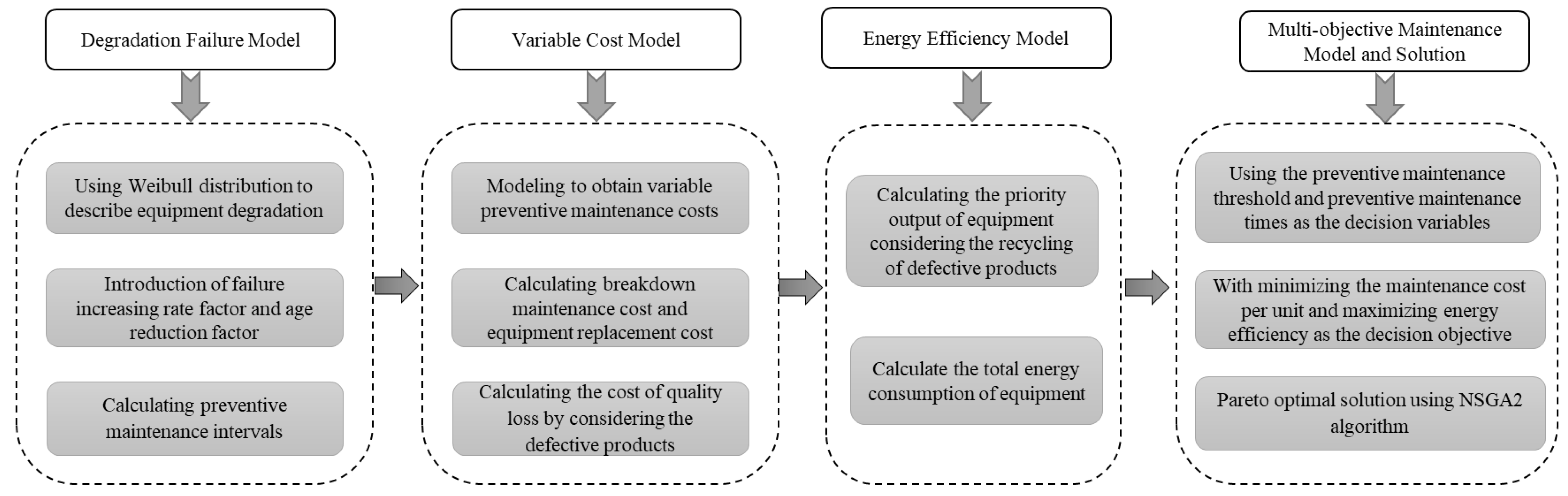
4. Modeling of the Maintenance Strategy Optimization

The multiobjective maintenance model considering equipment energy efficiency under the variable of cost is described as follows: first, the degradation failure model of equipment is developed by using the Weibull distribution and introducing the failure increasing rate factor and the age reduction factor to simulate the degradation process. Furthermore, based on the relationship between the reliability and failure rate, preventive maintenance intervals are calculated, which lays the foundation for the construction of equipment cost model and energy efficiency model. Then, the variable cost model is developed by considering the cost of different maintenance activities of equipment and considering the quality loss of the products produced by the equipment. Third, by calculating the energy consumption of equipment in each state to obtain the total energy consumption and introducing the recovery coefficient to obtain the effective output of equipment, the energy efficiency model of equipment is constructed. Fourth, the decision variables and optimization goals of the proposed model are determined to build a multiobjective decision-making model. Finally, the NSGAII algorithm is selected, and the model is solved based on the algorithm process. The modeling of the maintenance strategy optimization process is shown in Figure 2.

4.1. Degradation Failure Model

The performance of equipment is continuously degrading as equipment operates. The Weibull distribution is widely used to simulate the cumulative failure analysis of mechanical and electrical equipment. In this paper, the Weibull distribution is used to describe the degradation level of equipment. The failure rate function at running time t is expressed as:

$$\lambda (t)=\frac{\beta }{\alpha }{(\frac{t}{\alpha })}^{\beta -1}$$

(1)

where $\alpha ,\beta$ are the scale parameters and shape parameters of the Weibull distribution, respectively, which are obtained from the historical maintenance data of equipment. As the health rate of equipment cannot be restored to a new state after preventive maintenance, the failure rate increasing factor $b_i(b_i>1)$ and service age decreasing factor $a_i(0<a_i<1)$ are introduced to express the change in the failure rate. The failure rate increasing factor indicates that the equipment failure rate at each operating moment will increase after preventive maintenance. The service age decreasing factor indicates that the health state of equipment after preventive maintenance will return to a state between the new state and the state before adopting maintenance. The failure rate expression of equipment after the ith preventive maintenance can be obtained:

$${\lambda }_{i+1}=b_i{\lambda }_i(t+a_i{T}_{\mathrm{i}})$$

(2)

There is a certain relationship between the reliability of equipment and the failure rate function. When the equipment reaches the preventive maintenance threshold $R^{\ast }$, preventive maintenance will be carried out. Assuming that N times of preventive maintenance are carried out, each preventive maintenance interval can be obtained:

$$e^{-{\displaystyle {\int }_0^{T_i}{\lambda }_i(t)dt}}=R^{\ast } i=\{1,2,\dots ,N\}$$

(3)

where $T_i$ represents the operational time of equipment from i − 1th preventive maintenance to ith preventive maintenance.

4.2. Variable Cost Model

In this section, the maintenance cost in each condition is calculated, and the quality loss of the defective products produced is considered. Then, the total cost is divided by the cycle time to obtain the maintenance cost per unit, which is obtained by dividing the total cost by the cycle time T. In this paper, the total maintenance cost is mainly composed of preventive maintenance cost, breakdown maintenance cost, replacement cost, and quality loss cost.

(1)

Preventive maintenance cost

According to the assumption of the model, when the reliability of equipment reaches the threshold of preventive maintenance, preventive maintenance will be carried out. In previous research, the cost of preventive maintenance was fixed. However, the cost of preventive maintenance cannot be fixed due to the deteriorating performance of equipment. When equipment performance significantly deteriorates, it will inevitably cost more to maintain. It means that the cost of preventive maintenance will continue to increase with the degradation of equipment, which is fluctuating. Thus, the cost of ith preventive maintenance of equipment is composed of both fixed costs and variable costs, and it is expressed as:

$$C_{\mathrm{m}}^{pmi}=C_s^{pm}+C_{vi}^{pm}=C_s^{pm}+\gamma {\lambda }_i(T_i)$$

(4)

where $C_s^{pm}$ represents the fixed cost of preventive maintenance, $C_{vi}^{pm}$ represents the variable cost of ith preventive maintenance, which is linearly related to the amount of equipment degradation indicated by ${\lambda }_i(T_i)$, and the correlation coefficient is $\gamma$.

Assuming that the maintenance time for each preventive maintenance is $t_m^{pm}$, the total cost and total time of preventive maintenance in the cycle is therefore expressed as:

$$T{C}_{\mathrm{m}}^{pm}={\displaystyle \sum _{i=1}^N{C}_m^{pmi}=}{\displaystyle \sum _{i=1}^N{C}_s^{pm}+\gamma {\lambda }_i(T_i)}$$

(5)

$$T_{\mathrm{m}}^{pm}=N\times t_m^{pm}$$

(6)

(2)

Breakdown maintenance cost

According to assumption 1, the total cost of breakdown maintenance is equal to the number of failures multiplied by each breakdown maintenance cost. The number of failures in a preventive maintenance cycle can be calculated from Equation (3), which is expressed as:

$$N_c^i={\displaystyle {\int }_0^{T_i}{\lambda }_i(t)dt}=-\ln R^{\ast }$$

(7)

The time and cost of each breakdown maintenance are $t_m^{pm},C_m^{cm}$, respectively. The total time and total cost of breakdown maintenance can be obtained according to Equation (7):

$$T{C}_{\mathrm{m}}^{cm}=C_m^{cm}\times ((N+1)\times (-\ln R^{\ast }))$$

(8)

$$T_{\mathrm{m}}^{cm}=t_m^{cm}\times ((N+1)\times (-\ln R^{\ast }))$$

(9)

(3)

Quality loss cost

Generally, equipment will produce a certain amount of substandard products during the production process. Most of these substandard products can be caused by equipment designed so that it cannot be reduced, and some are caused by equipment degradation. The cost of quality loss is the loss of inferior products that cannot be sold properly due to quality problems. With the degradation of equipment, the product quality will continue to degrade. At this time, the number of defective products will continue to increase, resulting in a particular cost. According to past sales data, the revenue of each product can be measured, and the cost of quality loss can be measured by the original sales revenue of defective products. Thus, it is necessary to calculate the number of defective products closely related to the defective product rate. According to Assumption 5, the defective rate of equipment varies, and it can be expressed as:

$$p({\lambda }_i(t))=p_0+\mu [1-e^{-\sigma {\lambda }_i{(t)}^{\theta }}]$$

(10)

where $p_0$ represents the defective rate in the new state of equipment,$\mu$ represents the boundary of quality deterioration, and $\sigma$ and $\theta$ are constants [36].

Assuming that the loss cost of a single product is $C_v^d$, and the production rate is v, the quality loss cost of equipment in the period T is:

$$T{C}_d=C_{dv}\times {\displaystyle \sum _{i=1}^{N+1}{T}_{\mathrm{i}}\times v\times {\overline{p}}_i}$$

(11)

In Equation (11), ${\overline{p}}_i$ represents the average defective rate of products produced by equipment during i − 1th and ith preventive maintenance intervals. The calculation equation of the average defective rate is as follows:

$${\overline{p}}_i=\frac{p({\lambda }_i(0))+p({\lambda }_i(T_i))}{2}$$

(12)

According to Assumption 3, replacement cost and time are $C_r$ and $T_r$, respectively.

Currently, the total cost of equipment can be obtained. The next cycle time needs to be calculated. As is shown in Figure 1, the period T from the new state of equipment to the next replacement is composed of preventive maintenance time, equipment normal operation time, breakdown maintenance time, and replacement time. Finally, based on the above analysis, the variable cost model can be developed expressed by the maintenance cost per unit obtained by dividing the total cost during the cycle time T. The expression is as follows:

$$\begin{array}{cc}ETC& =\frac{T{C}_m^{pm}+T{C}_m^{cm}+C_r+T{C}_d}{{\displaystyle \sum _{i=1}^{N+1}{T}_i}+T_m^{pm}+T_m^{cm}+T_r}\\ & =\frac{{\displaystyle \sum _{i=1}^N{C}_s^{pm}+\gamma {\lambda }_i(T_i)}+C_m^{cm}\times ((N+1)\times (-\ln R^{\ast }))+C_r+{\displaystyle \sum _{i=1}^{N+1}{C}_{dv}\times v\times {\overline{p}}_i\times T_i}}{{\displaystyle \sum _{i=1}^{N+1}{T}_i}+N\times t_m^{pm}+T_r+t_m^{cm}\times ((N+1)\times (-\ln R^{\ast }))}\end{array}$$

(13)

4.3. Energy Efficiency Model

The key to achieving carbon neutrality lies in energy conservation and emission reduction. In order to achieve energy conservation and emission reduction, it is necessary to explore the problem of excessive energy consumption in the process of product production and equipment maintenance and to improve energy efficiency. Energy efficiency is an important indicator to measure the input–output ratio of the manufacturing industry. The energy efficiency in the manufacturing process is expressed as the ratio between the total output capacity and the total input energy [37]. Thus, in order to obtain the energy efficiency of equipment, the total energy consumption and the total effective output of equipment need to be calculated. The first step is to find out the energy consumed by equipment. It is common knowledge that the energy consumption of equipment in different states varies. According to the difference, the state of equipment can be divided into normal operation state, standby state, warm-up state, power-on state, and power-off state. Since the time of power-on and power-off is very short, the energy consumption is negligible. The energy consumption of equipment is shown in Figure 3.

The energy consumption considered in this paper includes two parts, the energy consumption of equipment and the energy consumption of maintenance. The energy consumption of equipment includes the energy consumption of the normal operation, the standby energy consumption, and the warm-up energy consumption. The maintenance energy consumption is mainly the energy consumption of three maintenance activities. The various energy consumptions are calculated below.

(1)

Operation energy consumption of equipment

The energy consumption of equipment during operation increases with degradation, which is linearly related to the failure rate. The energy consumption per unit before ith preventive maintenance is expressed as:

$$X_i(t)=X_0+\omega {\lambda }_i(t)$$

(14)

where $X_0$ represents the energy consumption of equipment at the initial stage, and $\omega$ represents the linear relationship between the variation of equipment energy consumption and equipment failure rate. Thus, the total operation energy consumption of equipment in period T is expressed as:

$$E_o={\displaystyle \sum _{i=1}^{N+1}{\displaystyle {\int }_0^{T_{\mathrm{i}}}{X}_i(t)dt}}={\displaystyle \sum _{i=1}^{N+1}{\displaystyle {\int }_0^{T_i}{X}_0+\omega {\lambda }_i(t)}}dt$$

(15)

(2)

Standby energy consumption of equipment

According to Assumption 2, equipment is on standby while preventive maintenance is being performed. The standby time of equipment can be measured by the preventive maintenance time. Assuming that the standby energy consumption per unit of equipment is $E_{\mathrm{iv}}$, the total standby energy consumption can be expressed as:

$$E_{\mathrm{i}}=E_{iv}\times T_m^{pm}=E_{iv}\times N\times t_m^{pm}$$

(16)

(3)

Warm-up energy consumption of equipment

According to Assumption 4, the equipment needs to go through a warm-up time after it is turned on. The equipment needs to be shut down for maintenance and replacement. Assuming that the energy required to warm up equipment once is $E_{wv}$, then the total warm-up energy consumption of equipment is expressed as:

$$E_w=E_{wv}\times {\displaystyle \sum _{i=1}^{N+1}{N}_c^i}=E_{wv}\times ((N+1)\times (-\ln R^{\ast }))$$

(17)

(4)

Equipment maintenance energy consumption

When equipment performs maintenance activities, it needs to consume other energy such as electricity. Assuming that the energy consumption of each breakdown maintenance and preventive maintenance is $E_{pv}$, and the energy consumption of equipment replacement is $E_{pr}$, then the maintenance energy consumption of equipment in the period T is:

$$E_p=E_{pv}\times (N+(N+1)\times (-\ln R))+E_{pr}$$

(18)

The above equation has calculated the total energy consumption of equipment, and then the total effective output of equipment needs to be obtained. The total effective output of equipment includes qualified products and defective products that can be recycled. With the deterioration of equipment, the defective rate is increasing, and the recovery factor will change correspondingly. The recovery factor ${\tau }^i$ is introduced to describe the gradual decrease in the amount of recovery. Thus, the final effective output of equipment is obtained by subtracting the number of defective products that cannot be recovered and is expressed as:

$$Y={\displaystyle \sum _{i=1}^{N+1}{T}_i}\times v-{\displaystyle \sum _{i=1}^{N+1}v\times {\overline{p}}_i\times T_i\times (1-{\tau }^i)}$$

(19)

The final energy efficiency model can be obtained and expressed as:

$$\begin{array}{cc}EE& =\frac{Y}{E_o+E_i+E_w+E_p}\\ & =\frac{{\displaystyle \sum _{i=1}^{N+1}{T}_i}\times v-{\displaystyle \sum _{i=1}^{N+1}v\times {\overline{p}}_i\times T_i\times (1-{\tau }^i)}}{{\displaystyle \sum _{i=1}^{N+1}{\displaystyle {\int }_0^{T_i}{X}_0+\omega {\lambda }_i(t)}}dt+E_{iv}\times N\times t_m^{pm}+E_{wv}\times ((N+1)\times (-\ln R^{\ast }))+E_{pv}\times (N+(N+1)\times (-\ln R))+E_{pr}}\end{array}$$

(20)

4.4. Multiobjective Maintenance Model

In order to achieve a balance between the economic benefits and social benefits of the enterprise, not only maintenance costs but also energy efficiency need to be considered. Thus, this paper aims to minimize the maintenance cost per unit and maximize energy efficiency, using the preventive maintenance threshold and preventive maintenance times as the decision variables. In addition, a multiobjective maintenance model can be constructed. The expression is as follows:

$$D=\{\begin{array}{l}\min ETC(R^{*},N^{*})\\ \max EE(R^{*},N^{*})\end{array}$$

(21)

4.5. Solution of the Maintenance Strategy Optimization

NSGAII is a multiobjective genetic algorithm widely used to analyze and solve multiobjective optimization problems due to its advantages of fast solution speed and good convergence of solutions. In this paper, the relationship between energy efficiency and cost per unit needs to be reconciled to satisfy each objective as far as possible. For this reason, the NSGAII algorithm is used to solve the model; the model solution process is shown in Figure 4. Its processes are as follows.

Step 1:

Parameter input. Input relevant parameters of the algorithm such as the number of populations, the maximum number of iterations, upper and lower bounds on the preventive maintenance threshold, crossover rate, and variation rate. Initialize the population and generate a random population P of N individuals.

Step 2:

Calculate the maintenance cost and energy efficiency per unit for each individual in the population.

Step 3:

Fast nondominated sorting. The individuals in the population P are classified by the fast nondominated sorting algorithm. According to the dominance relationship between the objective function values, the current optimal solution is selected and marked as rank 1. Then after excluding the solutions in the dominant rank 1, the optimal solution is selected from the remaining population and marked as rank 2, and so on, until the whole population is graded. The nondominated solution sets of different levels are constructed, such as F₁, F₂, … F_n. As the optimization objective of this paper is to minimize the maintenance cost per unit and maximize energy efficiency, when the target value of energy efficiency is the vertical coordinate, and the target value of maintenance cost per unit is the horizontal coordinate, the higher the rank of the points on the axis to the upper left.

Step 4:

Crowding distance calculation. In order to select the better individuals of the population and prevent falling into local maxima and local minima, the crowding distance of individuals needs to be calculated. It is defined as the sum distance of the two points on either side of this point along each of the objectives, denoted by i_d. As shown in Figure 5, the crowding distance of the ith point is expressed as the sum of the variable lengths of the rectangular rectangle, that is, the sum of the distance along the direction of the first objective and the distance along the direction of the second objective. The formula is expressed as:

$$i_d=[f_1(i+1)-f_1(i-1)]+[f_2(i-1)-f_2(i+1)]$$

(22)

Step 5:

Elite retention strategy. In order to prevent the loss of outstanding individuals during the evolution of the population, an elite retention strategy for individuals is required. The total crowding distance for each individual is equal to the sum of the distances for each single target metric. According to the elite retention strategy, individuals are selected sequentially from the highest ranked nondominated solution set to the lower ranked solution set. If two individuals are in the same rank, the crowding distance between them is compared, and the individual with the greater crowding is selected. N individuals are eventually selected to form a new parent population Q.

Step 6:

Determine if the maximum number of iterations has been reached. If the maximum number of iterations is reached, the Pareto solution set is output; if not, the new parent population Q is crossed and mutated, the resulting child population Q′ is merged with the parent population Q, and the operation in Step 2 is repeated.

5. Case Study

5.1. Data Preparation

The validity and adaptability of the multiobjective decision model are verified by a case study. In this paper, the production equipment of a manufacturing company is selected for the study. The production equipment produces products at a fixed rate every day. The equipment will produce a small number of defective products that can be recycled to a certain extent. Meanwhile, the defective product rate will increase with equipment degradation, and equipment operation and maintenance consume more energy. Referring to the historical data of the equipment, it can be found that the failure rate of the equipment obeys the Weibull distribution with the shape parameter of 3 and the size parameter of 110, and then referring to the general calculation of comprehensive energy consumption, the following parameters related to maintenance and energy consumption are obtained. As the types of products produced by the equipment will change with customer demand, the defective data of each product varies. In this paper, one of the products is selected, and the initial defective rate is obtained by analyzing the defective data. Other parameters of defective products are determined by referring to the literature [36]. Furthermore, due to the change in customer demand, the production rate of the equipment is not fixed. We assume that the production rate of the equipment is 100 pieces per day, thus obtaining the total parameter table, as shown in

Table 1. Value of related parameters.

Maintenance Parameters		Energy Consumption Parameters		Production Parameters
$C_s^{pm}$	400	$x_0$	180	$P_0$	0.008
$C_{mv}^{cm}$	150	$\omega$	1.2	$\mu$	0.075
$C_{dv}$	10	$E_{iv}$	25	$\sigma$	20
$C_r$	2000	$E_{wv}$	15	$\theta$	1.1
$t_m^{pm}$	1	$E_{pv}$	50	$\tau$	0.4
$t_m^{cm}$	0.5	$E_{pr}$	300	$v$	100
$T_r$	2
$\gamma$	1.2

.

5.2. Results Analysis

In order to narrow the search for multiobjective solution sets and ensure the accuracy and convenience of the solution, the maintenance cost per unit and energy efficiency of equipment under different combinations of preventive maintenance thresholds and maintenance times were obtained by numerical simulation.

The results can be seen in Figure 6. When the preventive maintenance threshold is in the range (0.6, 0.8), and the number of preventive maintenance is in the range (0, 6), there is a minimum value of maintenance cost per unit and a maximum value of energy efficiency. In addition, the graph of simulation results shows that the maintenance cost per unit tends to decrease and then increase as the number of maintenance increases. When preventive maintenance is less frequent, the time from the beginning of use to the replacement of equipment is shorter, and the equipment maintenance cost is mainly composed of replacement cost and breakdown maintenance cost, which makes the maintenance cost per unit higher. With the increase in maintenance times, the cycle time will gradually become longer, while the maintenance cost slowly increases, and the maintenance cost per unit shows a downward trend. When the number of maintenance exceeds a certain threshold due to frequent maintenance, the preventive maintenance cost of equipment significantly increases, and the cycle time slowly increases at this time, which makes the maintenance cost per unit show an upward trend.

Similarly, energy efficiency tends to increase and then decrease as the number of maintenance increases. When the number of preventive maintenance times is small, the energy consumption of equipment maintenance is mainly composed of replacement energy consumption and operation energy consumption, which makes the increase in equipment output exceed the increase in energy consumption, and the energy efficiency shows an upward trend. When the number of maintenance times exceeds a certain threshold, the cycle will gradually become longer as the number of maintenance increases. At this time, the effective output of the equipment slowly increases, but the energy consumption rapidly increases due to frequent preventive maintenance and breakdown maintenance, which makes the energy efficiency show a downward trend.

The optimal solution for the single objective can be obtained by conducting a simulation in the interval of the preventive maintenance thresholds of (0.6, 0.8) and the preventive maintenance times of (0, 6), as shown in

Table 2. Simulation results for maintenance costs per unit.

R	N = 0	N = 1	N = 2	N = 3	N = 4	N = 5	N = 6
0.6	30.733	28.83966	26.97263	26.50926	26.65826	27.13605	27.80899
0.61	30.85359	28.80936	26.91436	26.43532	26.57268	27.04048	27.7043
0.62	30.98098	28.78345	26.85985	26.36491	26.49058	26.9484	27.60315
0.63	31.11558	28.76212	26.80925	26.29816	26.41207	26.85993	27.50566
0.64	31.25781	28.74557	26.76272	26.23523	26.3373	26.7752	27.41196
0.65	31.40815	28.73406	26.72046	26.17628	26.26642	26.69437	27.3222
0.66	31.5671	28.72785	26.68267	26.1215	26.19961	26.6176	27.23655
0.67	31.73525	28.72725	26.6496	26.07111	26.13707	26.5451	27.15522
0.68	31.91322	28.73258	26.62151	26.02533	26.07903	26.47708	27.07842
0.69	32.10173	28.74424	26.59871	25.98445	26.02574	26.41381	27.00641
0.7	32.30155	28.76263	26.58153	25.94877	25.97751	26.35557	26.93948
0.71	32.51357	28.78824	26.57036	25.91863	25.93465	26.30268	26.87794
0.72	32.73875	28.82161	26.56564	25.89444	25.89755	26.25552	26.82218
0.73	32.97822	28.86334	26.56786	25.87662	25.86664	26.2145	26.77261
0.74	33.2332	28.91411	26.57757	25.86571	25.84239	26.1801	26.72972
0.75	33.50512	28.97472	26.59542	25.86226	25.82536	26.15288	26.69407
0.76	33.79558	29.04606	26.62213	25.86696	25.81621	26.13348	26.66628
0.77	34.10643	29.12916	26.65856	25.88057	25.81566	26.12261	26.6471
0.78	34.43977	29.22522	26.70568	25.90398	25.82457	26.12114	26.63738
0.79	34.79807	29.3356	26.76462	25.93823	25.84395	26.13004	26.63811
0.8	35.18419	29.46194	26.83671	25.98453	25.87495	26.15049	26.65046

and

Table 3. Simulation results for energy efficiency.

R	N = 0	N = 1	N = 2	N = 3	N = 4	N = 5	N = 6
0.6	0.540185	0.542253	0.542420	0.542160	0.541726	0.541198	0.540612
0.61	0.540153	0.542267	0.542452	0.542204	0.541779	0.541258	0.540678
0.62	0.540119	0.542279	0.542483	0.542245	0.541829	0.541315	0.540743
0.63	0.540081	0.542289	0.542511	0.542285	0.541877	0.541371	0.540805
0.64	0.540040	0.542296	0.542538	0.542323	0.541924	0.541425	0.540865
0.65	0.539995	0.542301	0.542562	0.542359	0.541968	0.541476	0.540923
0.66	0.539946	0.542303	0.542584	0.542392	0.542010	0.541525	0.540978
0.67	0.539894	0.542303	0.542603	0.542424	0.542050	0.541572	0.541032
0.68	0.539837	0.542299	0.542620	0.542452	0.542087	0.541617	0.541082
0.69	0.539775	0.542292	0.542634	0.542478	0.542122	0.541658	0.541130
0.7	0.539708	0.542282	0.542646	0.542502	0.542154	0.541697	0.541176
0.71	0.539636	0.542269	0.542654	0.542523	0.542183	0.541734	0.541218
0.72	0.539558	0.542251	0.542659	0.542540	0.542209	0.541767	0.541257
0.73	0.539474	0.542230	0.542660	0.542554	0.542232	0.541797	0.541293
0.74	0.539384	0.542204	0.542658	0.542565	0.542251	0.541823	0.541325
0.75	0.539286	0.542173	0.542652	0.542571	0.542267	0.541845	0.541353
0.76	0.539179	0.542137	0.542640	0.542574	0.542278	0.541863	0.541377
0.77	0.539064	0.542094	0.542624	0.542571	0.542285	0.541877	0.541396
0.78	0.538940	0.542046	0.542603	0.542564	0.542287	0.541885	0.541411
0.79	0.538804	0.541991	0.542576	0.542551	0.542283	0.541888	0.541419
0.8	0.538657	0.541927	0.542541	0.542532	0.542273	0.541885	0.541421

. The simulation results show that when the preventive maintenance threshold is 0.77 and the number of maintenance visits is 4, the lowest maintenance cost per unit is achieved at 25.81566. When the preventive maintenance threshold is 0.73 and the number of maintenance visits is 2, the highest equipment energy efficiency is achieved at 0.542660.

Thus, in this paper, we set the range of preventive maintenance threshold as (0.6, 0.8), the range of maintenance times as (2, 4), the number of individuals in the population as 100, the crossover rate as 0.9, the variation rate as 0.1, and the maximum number of iterations as 200. The above parameters were input into the algorithm of NSGAII, and the following results were obtained by a simulation using python, as shown in Figure 7. By comparing them, it is found that when N = 2, the energy efficiency of the equipment is the highest, but the maintenance cost per unit of equipment is also high. When N = 3, the energy efficiency of the equipment is lower than when N = 2, and the maintenance cost per unit of equipment is reduced more. When N = 4, the energy efficiency of the equipment is the lowest, but the maintenance cost per unit of equipment is not significantly reduced. Therefore, the comprehensive analysis yields that the energy efficiency and maintenance cost per unit of equipment is generally better for different maintenance thresholds at N = 3, so the Pareto curve at N = 3 is the final set of Pareto solutions for the model.

5.3. Results Comparison

Then, in order to verify the superiority of the model, a comparison with a single target is required. By comparing the results of the single objective decision with the multiobjective decision, we can see that when only the cost of maintenance is considered, the optimal solution is obtained with an objective value of (25.8157, 0.5423). It is clear that improvements in energy efficiency need to be made. When only energy efficiency is considered, the optimal solution obtained corresponds to an objective value of (26.5679, 0.5427), a decision that is clearly not optimal in terms of maintenance costs. In comparison, the compromise solution is (25.8622, 0.5426), where the energy efficiency is not much different from the single objective and the maintenance cost per unit is better, thus showing that the integrated consideration of maintenance cost and energy efficiency can help enterprises to achieve the goals of energy conservation and emission reduction.

5.4. Sensitivity Analysis

Finally, in order to analyze the relationship between the objective function and the parameters, this paper selects the maintenance cost parameters for sensitivity analysis by changing one maintenance cost parameter, keeping the other parameters constant, and observing the sensitivity of the objective function to the maintenance cost parameter. In this paper, the fixed cost of preventive maintenance, breakdown maintenance, and replacement cost affect the objective function. The range of parameter variation is −50~+50%. The analysis results obtained are shown in

Table 4. Sensitivity analysis results.

Parameters	Range of Changes	ETC	Variation of ETC	EE	Variation of EE
\	\	25.8622	\	0.5426	\
$C_s^{pm}$	−50%	22.9814	−11.15%	0.5422	−0.7%
	−25%	24.6962	−4.6%	0.5425	−0.2%
	+25%	26.9908	4.3%	0.5425	−0.2%
	+50%	28.0859	9.3%	0.5425	−0.2%
$C_m^{cm}$	−50%	25.5247	−1.3%	0.5425	−0.2%
	−25%	25.6952	−0.7%	0.5425	−0.2%
	+25%	26.0260	0.6%	0.5425	−0.2%
	+50%	26.1867	1.2%	0.5425	−0.2%
$C_r$	−50%	21.7022	−16.1%	0.5425	−0.2%
	−25%	23.8954	−7.6%	0.5425	−0.2%
	+25%	27.4742	6.2%	0.5422	−0.7%
	+50%	29.0641	12.4%	0.5421	−0.9%

.

According to the sensitivity analysis results, the maintenance cost per unit is more sensitive to the fixed cost of preventive maintenance and the replacement cost, and it varies positively with both parameters. When the fixed cost of preventive maintenance and the replacement cost decrease, the change in cost is more obvious than when they increase, which means that the maintenance costs per unit can be reduced by reducing the fixed costs of preventive maintenance and replacement costs when making maintenance decisions. In addition, the maintenance costs per unit and energy efficiency are not sensitive to breakdown maintenance cost, and changes in the fixed cost of preventive maintenance, breakdown maintenance cost, and replacement cost do not have a significant impact on changes in energy efficiency.

6. Conclusions

A methodological framework and a new preventive maintenance model were proposed that make it possible to optimize maintenance strategies in manufacturing production equipment. More generally, in the context of reducing carbon emissions and mitigating global warming, this paper focuses on solving the problem of equipment maintenance and energy efficiency in production systems by modeling and calculating the costs and various energy consumptions in the process of equipment maintenance to achieve the goal of optimizing maintenance strategies. In addition, the difference between considering energy efficiency and not is shown in this paper. The main findings of the article are the following: (1) compared with a maintenance strategy that only considers maintenance costs, the integrated consideration of maintenance costs, energy efficiency, and product quality is more suitable for manufacturing systems; (2) the modeling of dynamic preventive maintenance costs as well as dynamic operational energy consumption makes the calculation of costs and energy consumption more accurate; (3) the recycling of defective products is consistent with the goal of energy saving and emission reduction, and the amount of recycling is closely related to the state of the equipment. The framework and methods presented in this paper can be applied to production, maintenance, quality, and architecture maintenance optimization in manufacturing, which makes it possible to support management decisions. The decision process regarding production, quality control, and maintenance will be influenced by the results of the contribution. For example, the energy efficiency in maintenance will influence the maintenance policy, and the manufacturing system will specify new solutions for recycling defective products.

However, there are also limitations of the study. In many cases, manufacturing systems often include much equipment, which may be connected in series, parallel, or groups. The limitations of this paper, which considers only single-device preventive maintenance, also indicate potential directions for further research. In further research, the model can be extended to more complex equipment models and the use of opportunistic maintenance.