1. Introduction
The growing energy demand and development of various energy resources worldwide because of the increasing global population and industrialization have raised the amount of electrical power generated [
1]. Renewable energy is considered an alternative to fossil fuels. Importantly, renewable energy, such as solar, wind, hydroelectric, biomass, and geothermal energy, is replenishable and is directly procured from nature without environmental destruction.
Photovoltaic (PV) energy generation is a crucial component of renewable energy generation. PV energy is abundant, clean, and environment-friendly; further, it has experienced a gradual increase in use in recent years [
2,
3,
4]. Moreover, there is a significant acceleration in the installation of PV power generation systems worldwide. PV power generation involves directly converting solar energy into electrical energy. When solar rays are irradiated onto a semiconductor (
n- and
p-type silicon), electrons move between electrodes, generating electricity. Unlike fossil fuel power plants, the construction of a PV power plant is less complicated, emits zero pollution, and is environment-friendly [
5].
However, the power generated from a PV power plant can vary since it is affected by the construction location, time, panel capability, and size [
6,
7]. Moreover, intermittent variability of a PV power plant occurs depending on weather conditions, such as solar radiation, temperature, humidity, cloud cover, and wind speed, that are unpredictable and uncontrollable. Notably, changes in temperature and solar radiation can substantially affect power generation [
8,
9].
The nature of such variables can lead to unstable PV power generation, causing a sudden surplus or reduction in power output. Furthermore, it may cause an imbalance between power generation and load demand, inducing control and operation problems in the power grid [
10,
11]. If the amount of power generation can be accurately forecasted, operation optimization strategies, such as peak shaving and reducing the uncertainty of a power generation system, can be effectively applied [
12]. Therefore, a method for accurately predicting the amount of energy produced is crucial for PV-based power generation systems [
13,
14,
15]. Accurate forecasting can improve the quality of power provided to a power grid and help reduce the costs related to general variability [
16]. In addition, it can be used in various operation and control activities, including power scheduling in power distribution and transmission grids [
17].
Research on PV power generation forecasting has recently gained considerable interest. Primarily, studies that employ deep learning models are receiving increasing attention [
18,
19,
20]. Machine learning (ML)-based deep learning models were developed to solve complicated problems by extracting meaningful data from big data. Deep learning models are different from other theoretical ML models. Various hierarchical structures of deep learning models enable the automatic learning of the methods required to extract semantic features from raw data and find useful patterns.
Solar power generation has intermittent characteristics and is highly correlated with dependence on meteorological parameters. The use of various meteorological parameters can improve the forecasting accuracy of the model. Most conventional methods use multivariate regression, which requires collecting multiple relevant data such as solar radiation, temperature, and power generation. However, most PV plants in Korea have no environmental sensors installed owing to cost considerations; thus, the factors affecting PV power generation, such as temperature, humidity, cloud cover, and solar radiation, are challenging to identify. Therefore, only power generation data can be obtained. The Korea Meteorological Administration provides temperature and solar radiation data but it is not suitable for use due to location errors of PV plants. Motivated by this, we aim to present a deep model that forecasts power generation by analyzing time-series patterns in the data from a PV power plant at which environmental sensors are not installed.
We propose a hybrid model of a long short-term memory (LSTM) and convolutional neural network (CNN) model specialized for time-series data analysis and forecasting to improve the accuracy of power generation forecasting. The proposed network adopts a parallel structure of branched CNN-LSTM. First, a CNN offers the advantage of higher accuracy since different patterns can be identified depending on weather conditions based on the pattern extraction schemes. A proposed CNN model classifies the daily weather as sunny or cloudy by analyzing historical patterns in raw data. Then, the LSTM part is split into two models trained separately on sunny and cloudy day data and proceeds to extract long-term dependent features from the raw data. The LSTM model can more accurately predict the power generation by individually learning the power generation pattern according to each weather condition type.
The main purpose of this study is to enhance short-term PV forecasting accuracy by using the proposed hybrid model based on a univariate data approach. To train and evaluate the proposed method, using the power generation data collected from a PV power plant in Busan, Korea. The data were collected from 10 September 2019 to 22 July 2021. The data defined as corresponding to sunny and cloudy weather conditions by the Korea Meteorological Administration were used. The contributions obtained through the proposed method are as follows. We develop an accurate and simple CNN-LSTM model for PV forecasting that relies on historical PV data and does not rely on specific sensors or environment data.
The remaining paper is organized as follows.
Section 2 discusses previous studies on power generation forecasting algorithms. In
Section 3, the proposed hybrid CNN-LSTM model is introduced. The overview of the proposed analytical method, data cleaning, re-definition, and design verification of the LSTM model is presented. The performance of the proposed model is evaluated using objective indicators in
Section 4, and the conclusions are presented in
Section 5.
2. Related Work
A decrease in the PV module price, timely forecasting of power generation, and policies related to renewable energy have demonstrated a synergistic effect. Renewable-energy power plants are actively being constructed, thereby increasing energy production. Power generation forecasting plays a vital role from an economic perspective. Moreover, PV power generation forecasting helps rationally plan power generation to effectively solve problems such as system stability and power generation balance. The power generation forecasting of renewable energy using physical, statistical, ML, and artificial neural network (ANN)-based methods have been consistently researched.
Physical models forecast PV power generation based on numerical weather prediction (NWP) and physical principles of PV cells [
21]. An input of a physical model consists of dynamic information, such as NWP and environmental monitoring data, and static information, such as the installation angle of PV panels and the conversion efficiency of PV cells [
22]. Though the method does not require past information, it depends on geographic information of PV panels and detailed weather data.
Statistical methods set mapping relationships between past time-series data and PV energy outputs [
23]. The model performance depends on the relationship between past power generation observations and weather/climate parameters. Generally used statistical methods include autoregressive moving average, Kalman filter, and Markov chain [
24,
25,
26].
An ML method forecasts power generation by analyzing the correlations in nonlinear data. Such a method involves learning the characteristics of sample data and making predictions using a neural network or training model such as a support vector machine (SVM). The cross-validated model in [
27] used the characteristic statistical parameters of illumination intensity and surrounding temperature as the input vector. In [
28], a dataset corresponding to four different environments—sunny, cloudy, foggy, and rainy—was used. The model used an SVM and weather data to classify a specific environment and select an appropriate model to predict power generation. A hybrid ML model combining an SVM and the random forest algorithm was developed in [
29]. SVM predicts power generation, while the random forest was applied with an ensemble learning method wherein predicted values are combined and analyzed. Past and present generated power and weather data were combined as the input.
Artificial neural networks (ANNs), a subcategory of ML models, are widely used for forecasting [
30]. An ANN is a nonlinear model consisting of completely connected nodes. The node connections consist of weights used to analyze specific patterns within the data. An ANN predicts PV power generation through nonlinear approximation. An ANN-based prediction algorithm obtained favorable results using a shallow neural network in the initial steps. For the real-time prediction of PV solar energy, a hybrid method combining ANN and random forest has been proposed [
31]. An improved ANN model was successfully developed to enhance the PV energy forecasting accuracy [
32] despite uncertainty in solar radiation. Another study predicted power generation using solar radiation and panel temperature as independent variables [
33]. Furthermore, [
34] used the nonlinear characteristics of ANNs to predict solar radiation using multiple variables, such as average temperature, relative humidity, and daytime hours.
In recent years, numerous studies have been conducted on applying deep learning, which has shown excellent performance in diverse applications to power generation forecasting. Unlike ML algorithms, deep learning learns data and patterns using a complicated neural network architecture. The deep-learning-based recurrent neural network (RNN) is an ANN-type network that uses sequential or time-series data [
35]. This model uses information from the previous input to determine the current input and output. A feedback loop for the recurrent layer saves information about a point in time in the past time-series data of a memory cell. An RNN contains a shared parameter in each layer. A feed-forward network has different weights for each node, but an RNN shares the same weight parameter in each network layer. This weight is adjusted through backpropagation and gradient descent during training. Such characteristics of RNNs have been applied to PV power generation forecasting [
36,
37].
3. Proposed Method
3.1. CNN for Feature Extraction
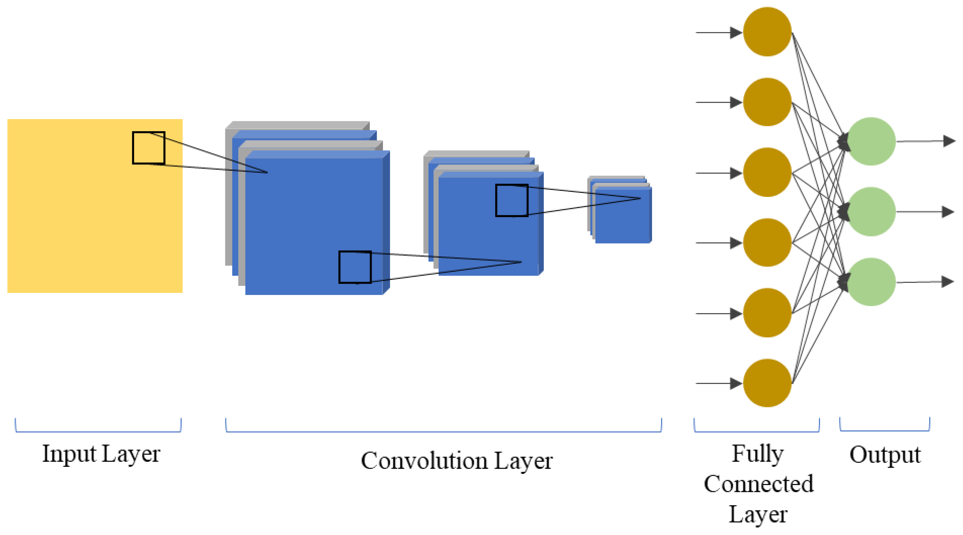
CNN, a deep learning algorithm frequently used for image, text, and signal inputs, consists of stacked layers that extract object features.
Figure 1 shows the basic architecture of a CNN.
The model performance is based on the number of stacked layers and the type and size of the kernel. The data in the input layer goes through convolution and pooling layers to extract deep features. These features are then input in the fully connected layer, where the result values are classified.
A CNN is used for extracting hierarchical features from an image. Accordingly, a CNN can extract important information from the one-dimensional sequential and two-dimensional input data.
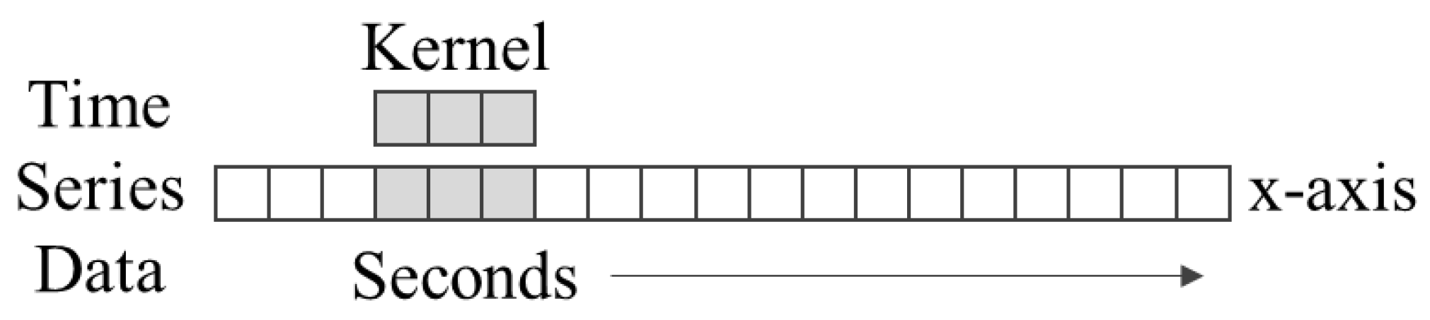
1D-CNNs are frequently used in natural language or time series processing since they can handle sequential data. Unlike in 2D-CNNs, the kernel executing convolution and the sequence of data being applied have a one-dimensional form in 1D-CNNs. As shown in
Figure 2, a 1D-CNN has a kernel moving along a single dimension.
3.2. Long Short-Term Memory
LSTM is one of the RNN architectures used for processing time-series data while solving the problem of gradient exploding or gradient vanishing. This network forgets unnecessary information while storing information for a prolonged time.
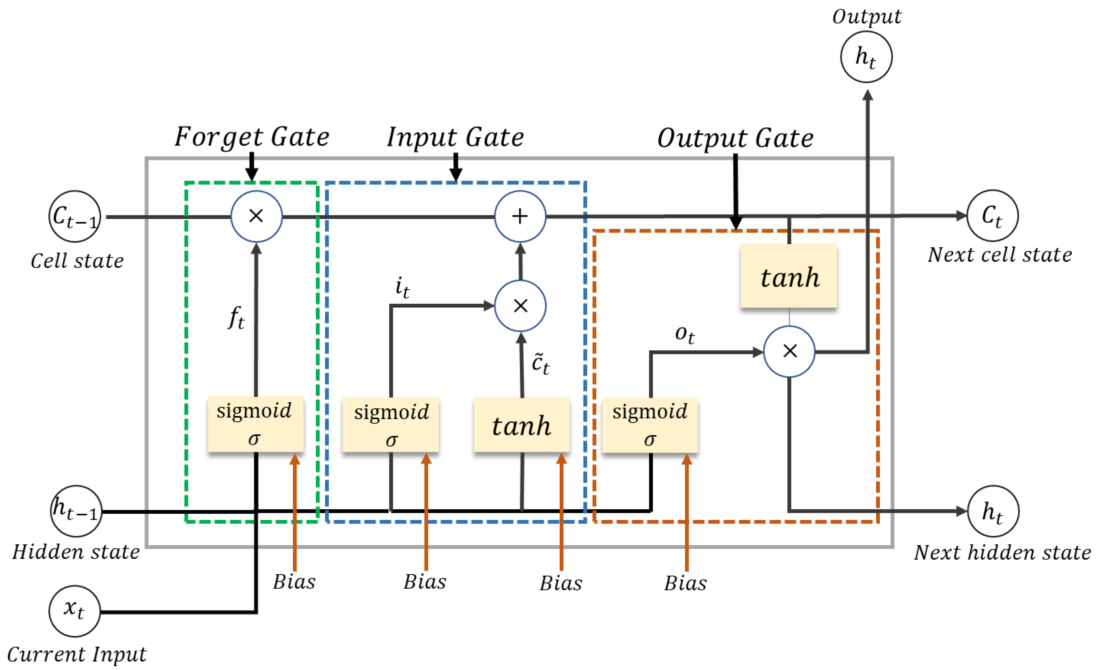
Figure 3 shows the cell structure of LSTM.
LSTM receives current input data and long- and short-term memory of the previous cell in each time step. Short-term memory represents the hidden state and represents , while long-term memory represents the cell state . A cell adjusts the information to be maintained or discarded in each time step before delivering short-term and long-term information to the next cell using a gate. This gate is called the input, forget, or output gate and accurately performs filtering through training.
The first step of LSTM is identifying and removing unnecessary information in a memory cell. This process is performed in the forget gate that determines an output value between 0 and 1 based on a sigmoid function. The closer the value is to 1, the more information about a previous state is maintained. The information of a previous state is forgotten as the value approaches 0, and omitted parts are decided. After passing the forget gate, the information to be stored is selected. If the previous time is forgotten, new information to be remembered is added, and the value of each element is decided as the newly added information. In this case, new information is not stored in the memory cell unconditionally; instead, an appropriate value is selected using an input gate.
The sigmoid function is added with the last LSTM cell and the current state and time activation feature. The value passed through the sigmoid layer is expressed as a number between 0 and 1 and indicates the degree of new information being updated. The value that has passed through the tanh function has a value between −1 and 1. Then, the output is multiplied, and the final value is stored in the long-term memory. The following process is used to select the output information. The output gate generates a new short-term memory (hidden state) to be delivered to the cell in the next step using the current input, previous short-term memory, and newly generated long-term memory. The output of the current time step can also be imported from the hidden state. The short- and long-term values generated by this gate are transferred to the next cell as the process is repeated. The output of each time step can be obtained from short-term memory or a hidden state.
Equations (1)–(6) are applied to each gate. Equation (1) shows the process of the forget gate. Input data are updated through Equations (2)–(4). The data undergo an operation, as in Equation (5), in the last output gate and are updated as per the final Equation (6). Here, is the sigmoid function, is the weight matrix, and represent the hidden and cell states, respectively.
3.3. Adaptive Selector
This paper proposed a hybrid CNN-LSTM model to forecast power generation. The CNN classifies weather type, while the LSTM predicts power generation. The LSTM model learns the power generation patterns according to weather type, which reduces the complexity and variability of data fitting to improve prediction accuracy.
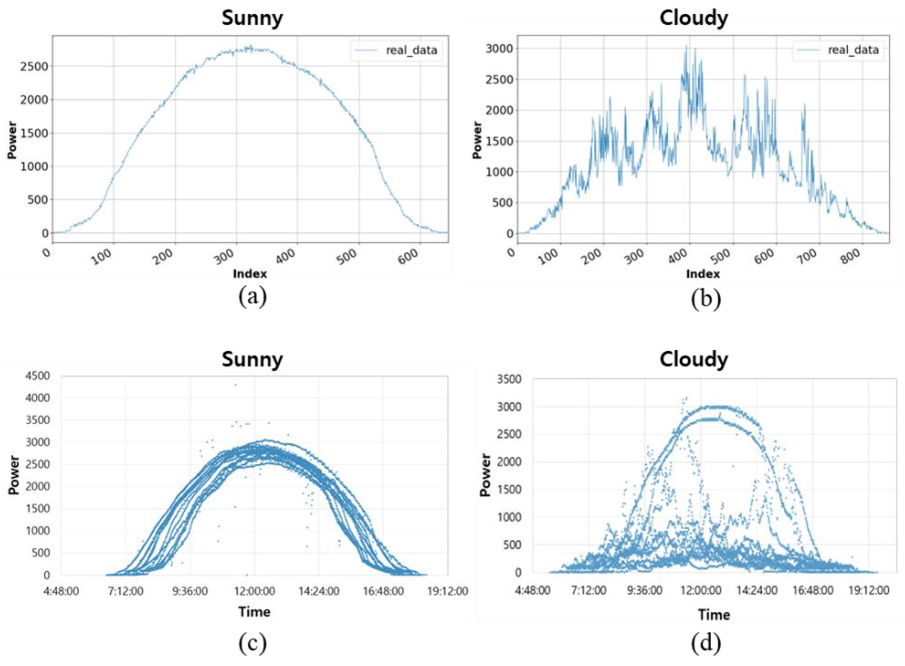
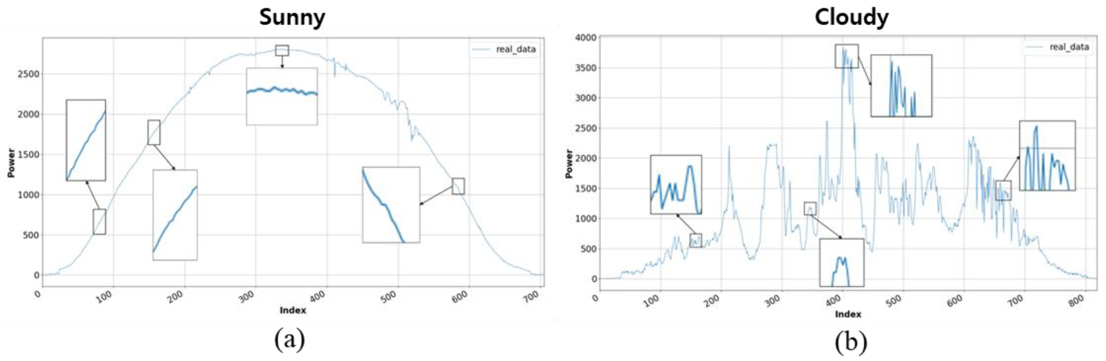
Figure 4 is the graph of power generation on sunny and cloudy days.
The power generation differs on a sunny and cloudy day, as shown in
Figure 4a,b, respectively. The power generation on a cloudy day is low and highly inconsistent. On a sunny day, the graph has a semi-circular data distribution affected by sunrise and sunset; the power generation is the highest around noon, as indicated by the high elevation. On a cloudy day, the variability of power generation is severe due to the changes in solar radiation.
Figure 4c,d shows that the power generation data on clear and cloudy days are superimposed and expressed as a scatter plot. In
Figure 4c, it can be seen that the power generation production pattern on a clear day is regularly generated within a certain area. In this figure, there are cases in which the power generation data is out of range by one point. This is an outlier due to equipment error or electrical noise. In
Figure 4d, it can be seen that the power generation pattern at the time of cloudy days has high variability according to the non-linear characteristics.
Figure 5a,b show the sectional power generation patterns during sunny and cloudy days, respectively. On a sunny day, the power generation gradually increases or decreases, but the variability abruptly changes on a cloudy day. Since such data patterns also influence continuous time-series patterns, using the LSTM model for training can complicate data convergence. Therefore, the current weather conditions are first classified according to the patterns in
Figure 5, and the power generation is forecasted using the individual LSTM model according to the classification results. Boxes in the
Figure 5 show the detailed pattern form of the collected power generation data. The data of sunny day is generated with a regular period, whereas data of cloudy day has a large fluctuation range and does not show periodicity. The proposed hybrid CNN-LSTM model is shown in
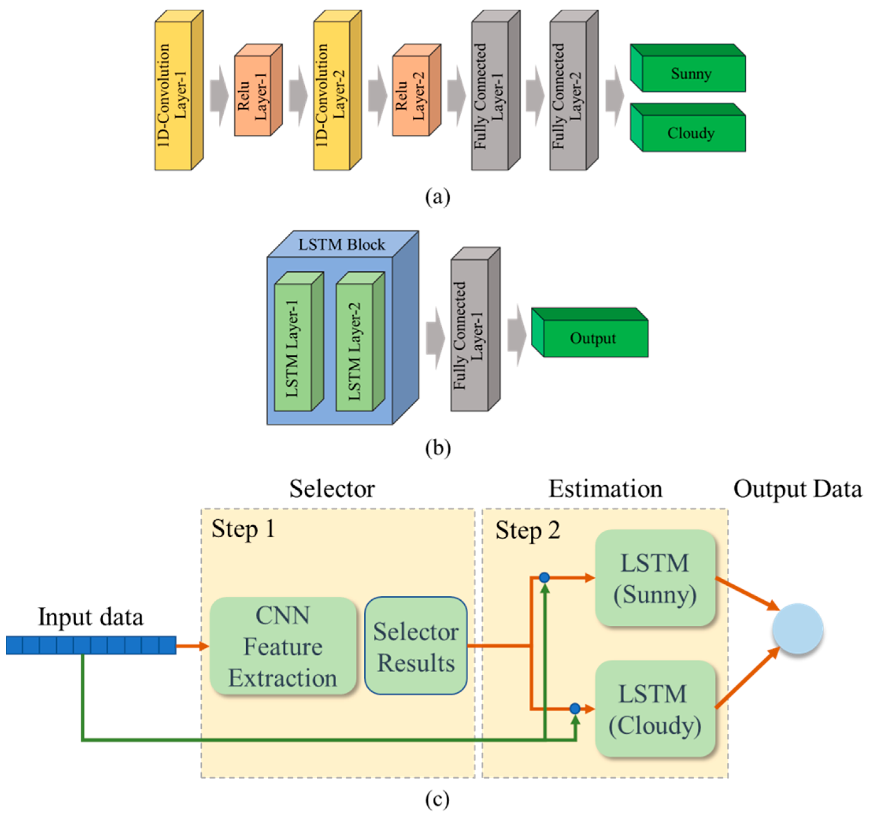
Figure 6.
Figure 6a shows the CNN architecture used to classify weather conditions. This architecture consists of two layers of convolution with relu layer and two layers of fully connected layers. The CNN model is trained to classify sunny and cloudy days based on the data pattern of weather conditions. The last layer outputs the results of the weather conditions. In the inner process of the neural network, the difference between the predicted values and the labels is calculated using a loss function. It then uses a backpropagation algorithm to minimize the loss function so that the predicted values are as close to the labels as possible. In the course of training a neural network, parameters, including weights and biases, are fine-tuned and updated to compare predicted values to labels to produce better predictions at every epoch. The optimizer used Adam and set learning rate = 0.01, the coefficient for primary momentum β1 = 0.9, the coefficient for secondary momentum β2 = 0.999, and epsilon = 10
−8. The weight initialization used kaiming uniform initializer and adopted the cross-entropy function as the loss function.
Figure 6b shows the LSTM architecture used to forecast PV power generation. This architecture consists of two layers of LSTM and one layer of the fully connected layer. The last layer outputs the predicted power generation. The two LSTM models with the same structure are trained on sunny and cloudy days data, respectively. In the case of the LSTM model, the input, forget and output gates and cell-state help the model to determine which values to preserve for keeping long-term memory during the computational process. The hyper-parameters used for network training are as follows. The optimizer used Adam and set learning rate = 0.001, the coefficient for primary momentum β1 = 0.9, the coefficient for secondary momentum β2 = 0.999, and epsilon = 10
−8. The weight initialization used kaiming uniform initializer and adopted MSE (Mean Square Error) function as the loss function.
Figure 6c shows the overall structure of the CNN-LSTM hybrid model. Select an LSTM model according to the output of CNN and predict PV power using time series data.
4. Experiment
In order to evaluate the effectiveness of the proposed deep model, we designed the following experiments using collected PV power datasets. The proposed hybrid model was trained and tested using the Python 3.8-based Pytorch deep learning framework as a software platform along with an AMD Ryzen 5 5600X CPU operating at 3.70 GHz, NVIDIA RTX 2070 GPU, and 16 GB RAM hardware environment.
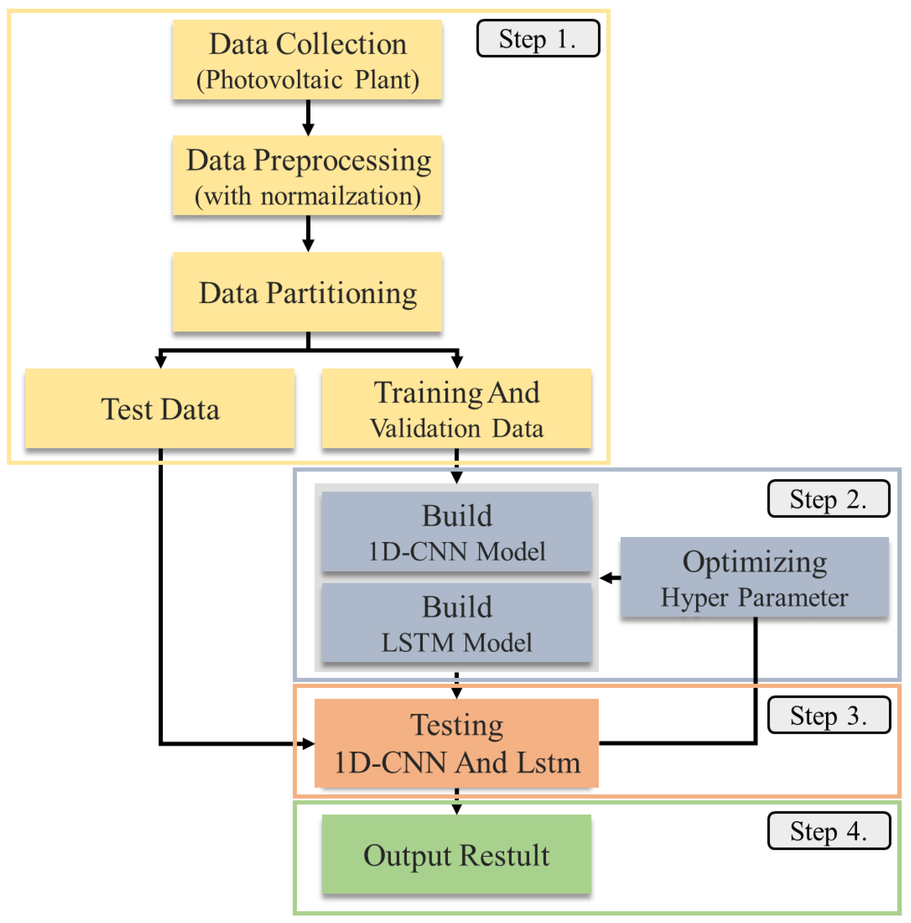
The proposed hybrid CNN- LSTM model performs PV power generation forecasting, as shown in
Figure 7. In step 1, the power generation data generated from a PV power plant are classified into sunny and cloudy day data. In step 2, the collected data are pre-processed to remove noise elements, such as missing values or outliers affecting the experiment. Normalization is then applied to use the data as a network input. In step 3, the CNN and LSTM are trained using the training data. Each model only uses power generation data. In step 4, the results of the forecasting model are tested and verified using various matrices.
4.1. Data Collection and Pre-Processing
This study used the power generation data collected from a PV power plant in Busan, Korea. The average annual PV power generation time of the region is 3.5 h, the average wind speed is 4–5 m/s, and the meridian altitude is 53° in spring (March–May), 76.5° in summer (June–August), 53° in fall (September–November), and 29.5° in winter (December–January). The data were collected from 10 September 2019 to 22 July 2021. The data defined as corresponding to sunny and cloudy weather conditions by the Korea Meteorological Administration were used. The Korea Meteorological Administration defines weather conditions in 11 steps. In this study, steps 1–5 were classified as sunny, while steps 6–11 were classified as cloudy [
38].
Table 1 presents the schema of the collected data.
Data and time in
Table 1 represented when the data were collected; cumulative power indicates cumulative power generation. The power generation data of 682 days were used for the experiment. The dataset consists of 446 and 236 sunny and cloudy day data points, respectively. Data imbalance may occur since the number of sunny day data is 1.88 times greater than the cloudy day data. Therefore, 100 data from each class were used for network training, while the remaining data were used for testing.
Abnormal elements in the input data of a forecasting model can cause high forecasting errors. Pre-processing the input data can improve model accuracy by reducing computation costs and solving the inappropriate training problem. PV power data sets can contain outliers due to solar equipment problems, collection system errors, and software system problems. Therefore, to eliminate outliers, the datasets are cleansing by calculating the 75% quantile.
The Cumulative power data in
Table 1 is preprocessed using the interquartile range (IQR). If the value of data was higher than that provided by Equation (7), it was determined as an outlier and removed.
Missing values in the collected data can occur due to problems in the inverter or data collection device. Since the proposed model predicts the data of a future point in time using continuous time-series data, missing values at can affect the model’s performance. Thus, time interpolation using the values at times and were applied.
The numerical scale of the power generation data used in this study is significant. For example, power generation is less than 10 W near 06:00 when the amount of solar radiation is low and more than 2500 W between 12:00–14:00 when the amount of solar radiation is the highest. A significant difference between the minimum and maximum values can affect the training speed and convergence accuracy of a network. Therefore, using Equation (8), normalization was performed to improve computation speed and accelerate the network training convergence speed.
Here, is the actual data, and z indicates a normalized value.
The data used in this study are the power generation data per minute, obtained by dividing the cumulative power generation data by power generation time. This study assumed a power plant without environmental sensors and predicted power generation using time-series analysis characteristics. Clouds and rain that occur locally reduce the amount of solar radiation, thus affecting the PV power generation efficiency. However, they are difficult to predict when environmental sensors are unavailable. Therefore, this study aimed to predict power generation based only on power generation patterns. The network receives 20 time-series data and outputs one data. The hyper-parameters used for training the network are as follows. The mean squared error (MSE) was used as the loss function, and the Adam optimizer was used for optimization. A learning rate of 0.01 was applied to network optimization.
4.2. Model Evaluation
In this study, a hybrid model combining CNN and LSTM is established. The general indicators used for evaluating the performance of a time-series data forecasting model include mean absolute error (MAE), root mean square error (RMSE), and mean absolute percentage error (MAPE). Let be the number of test data, be the value predicted by the proposed algorithm, and be the actual value in the quantitative indicators.
MAE measures the error between predicted and actual values and can vary depending on the measure of continuous variables, as shown in Equation (9). A smaller value indicates a higher accuracy.
RMSE, defined as in Equation (10), measures the difference between predicted and actual values; it is a measure of the deviation between predicted and actual values. An RMSE closer to 0 indicates better performance. The difference between RMSE and MAE is that RMSE is sensitive to outliers, making it more susceptible to significant deviation. Since the error is squared, a larger error leads to weight being reflected a greater extent.
MAPE, given by Equation (11), indicates the extent of error in the predicted value. A value closer to 0 can be interpreted as a more outstanding forecasting model performance. MAPE is robust to outliers, but in this case, it is more challenging to check for errors intuitively than in the case of MAE.
The power generation forecasted using the LSTM entails errors. The magnitude of errors varies depending on the density of the predicted power generation data. The error between predicted and actual values is smaller when the density of predicted values is dense. An error becomes more significant when the density is sparse. The accuracy of a forecasting model is also determined by density. As shown in Equation (12),
measures the strength of a correlation between the predicted and actual values.
has the range of
. A value closer to 0 indicates very low accuracy, and a value closer to 1 indicates higher accuracy of the forecasting model.
where
is the average of the actual power generation data.
4.3. Experimental Results
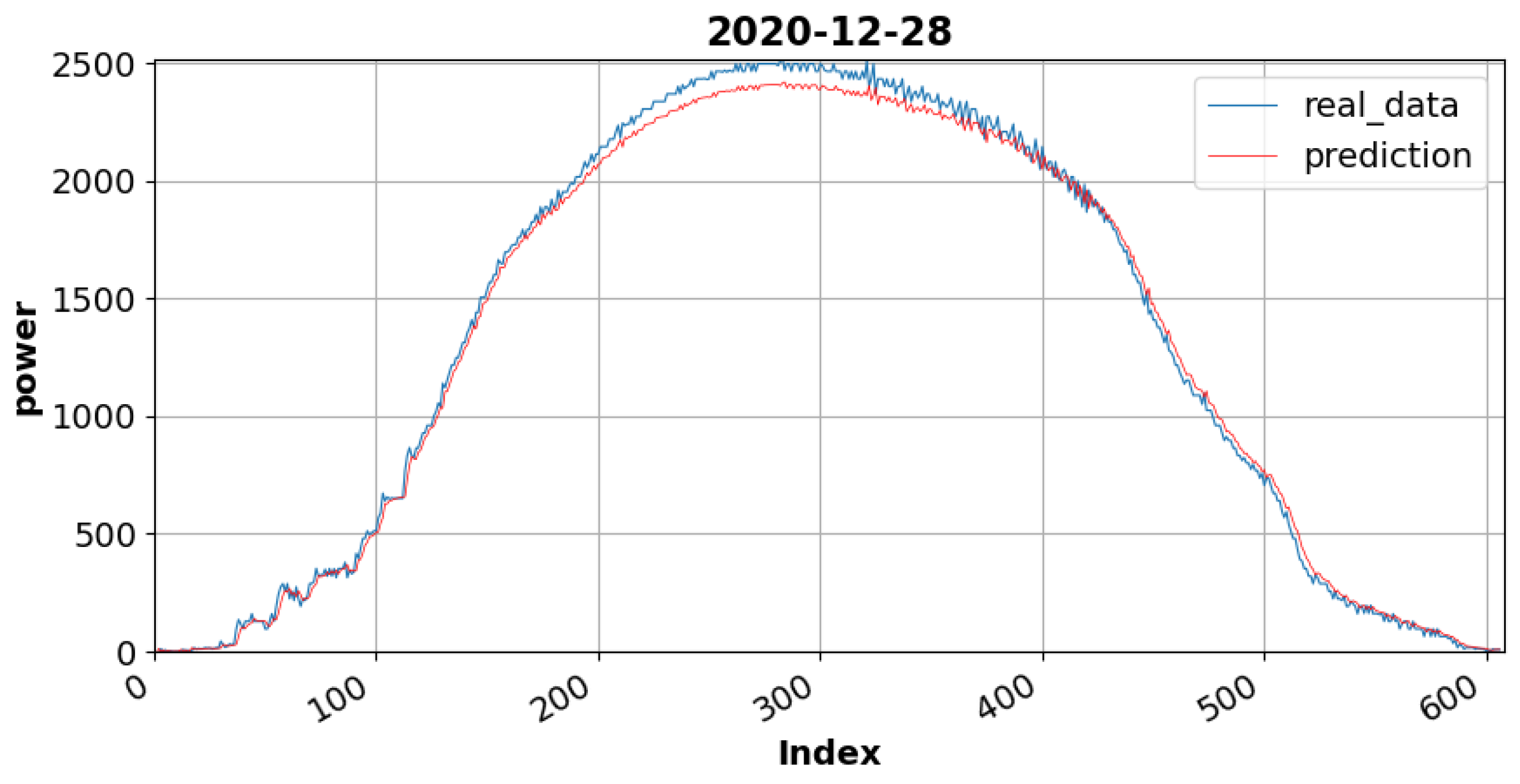
Quantitative and qualitative evaluations were performed using sunny and cloudy days’ data for model verification. The data of the same month (sunny day: 28 December 2020, cloudy day: 27 December 2020) were used for uniformity of the validation process.
Figure 8 is the graph of the sunny day dataset; certain sections demonstrate power generation fluctuations due to clouds.
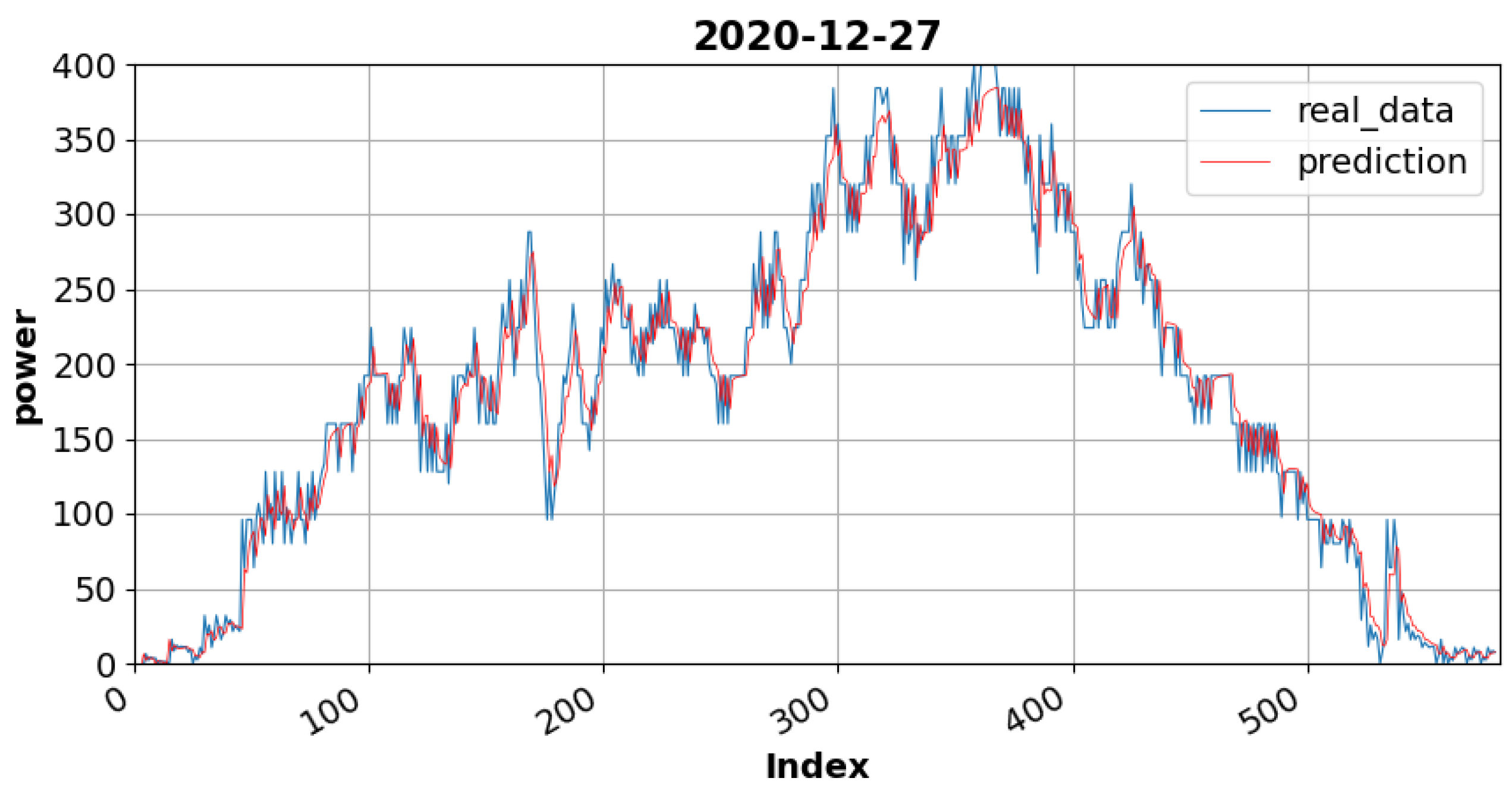
Figure 9 is the graph of the cloudy day dataset in which the maximum power output is 400 W. In contrast, on a sunny day, the maximum power output is 2500 W. This result implies that the amount of solar radiation is minimal, resulting in severe fluctuations in overall power generation. The blue line shows the measured data from the device, while the red line shows the prediction data. A quantitative evaluation was performed using MAPE, RMSE, and MSE to validate the LSTM forecasting model. The LSTM model adequately followed the trend of the observation data for accurate forecasting.
Table 2 presents the results of a quantitative evaluation of the test data for sunny and cloudy days. The sunny day data showed a MAPE of 4.58, which is lower than that of the cloudy day data, 7.06. In the cloudy day data, peak point errors occurred in the fluctuation amplitude according to the power production period, which increased the MAPE value compared to that of the sunny day data. The RMSE and MAE were lower in the cloudy day data, thus exhibiting more outstanding results.
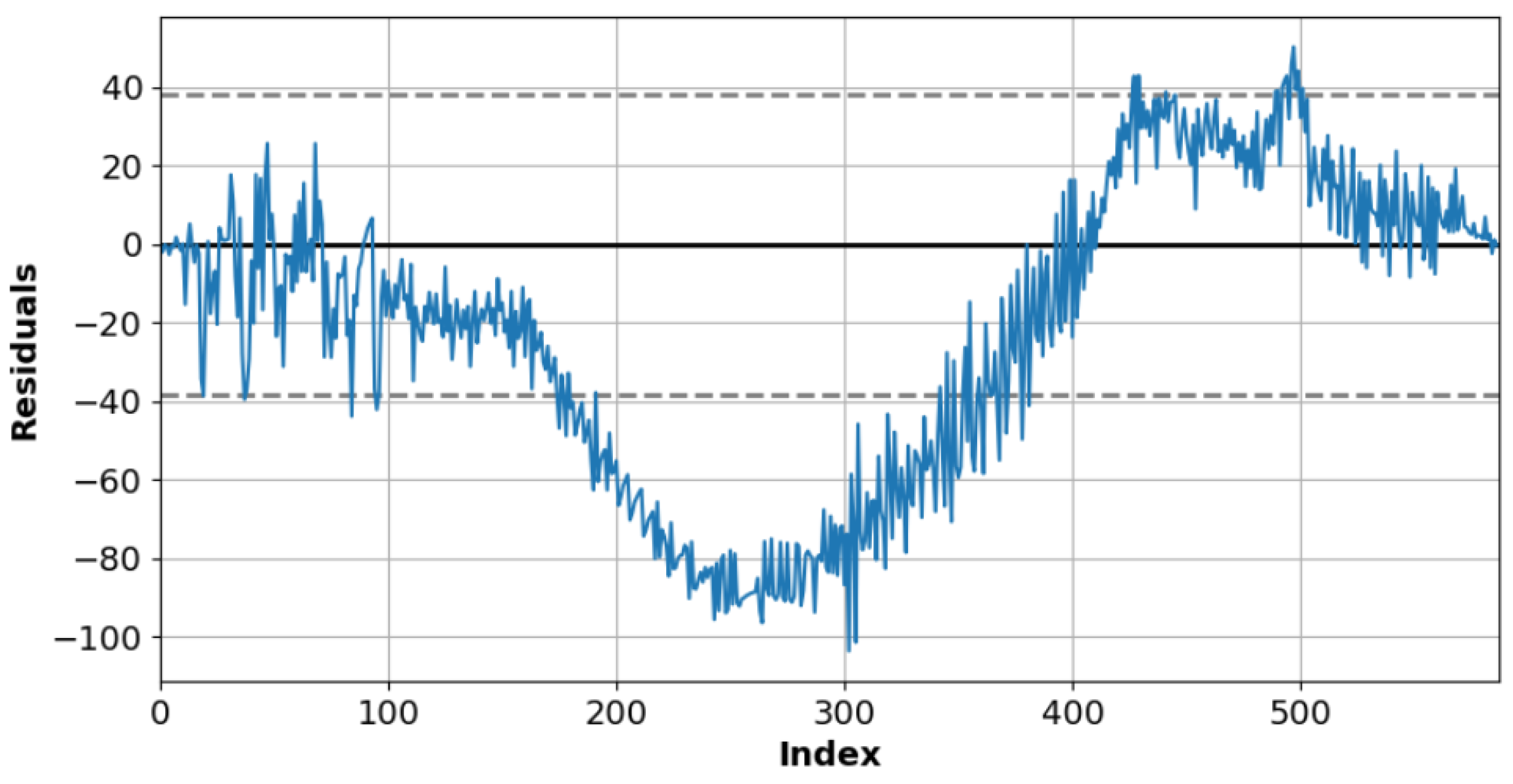
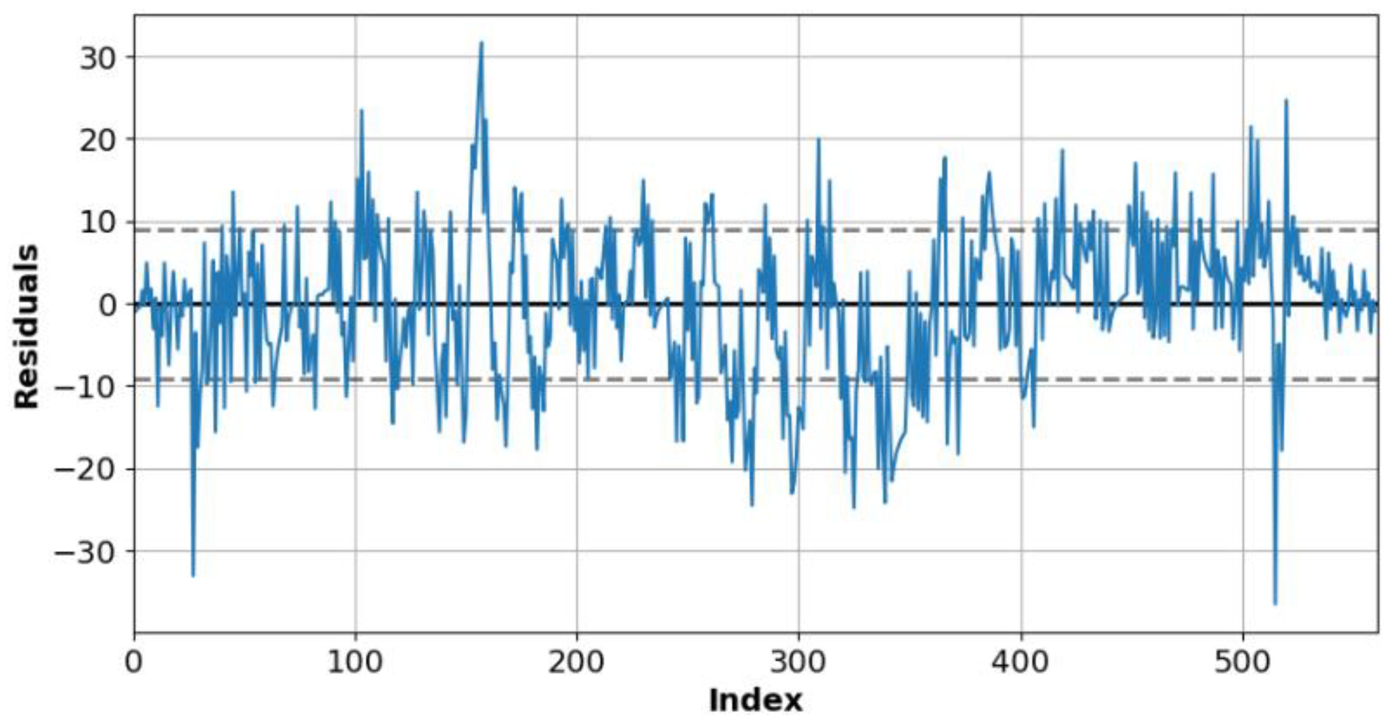
Figure 10 and
Figure 11 plot the residuals between observed and forecasted values for the sunny and cloudy day test data. The dotted line indicates the standard deviation (SD) corresponding to the residuals.
Table 3 presents the residual comparison results for a sunny day. The SD of residual is 38.25, and the mean is 34.00 on a sunny day.
Table 4 presents the residual comparison results of a cloudy day. The SD of residual is 27.42, and the mean is 17.13 on a cloudy day. A relatively large number of the residual values of sunny days deviate from the standard deviation section for the number of data, which can be observed between index 200 and 400 in
Table 3. This section is the peak point region where the power generation is the largest in
Figure 8.
The forecasting model can generate errors in predicting the maximum power generation value. The error in the cloudy day data is 10.83 less than that for the sunny day data. The number of data deviating from the standard deviation section is less than the number of data used in the experiment.
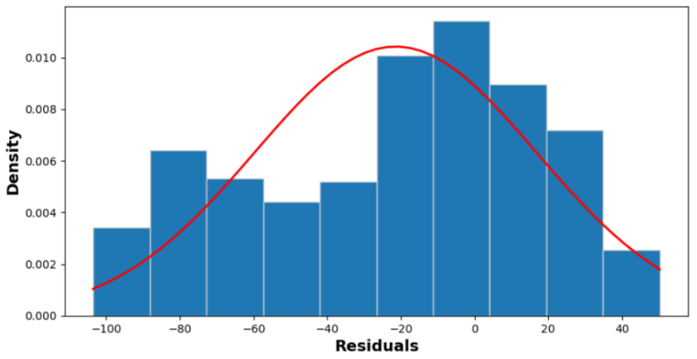
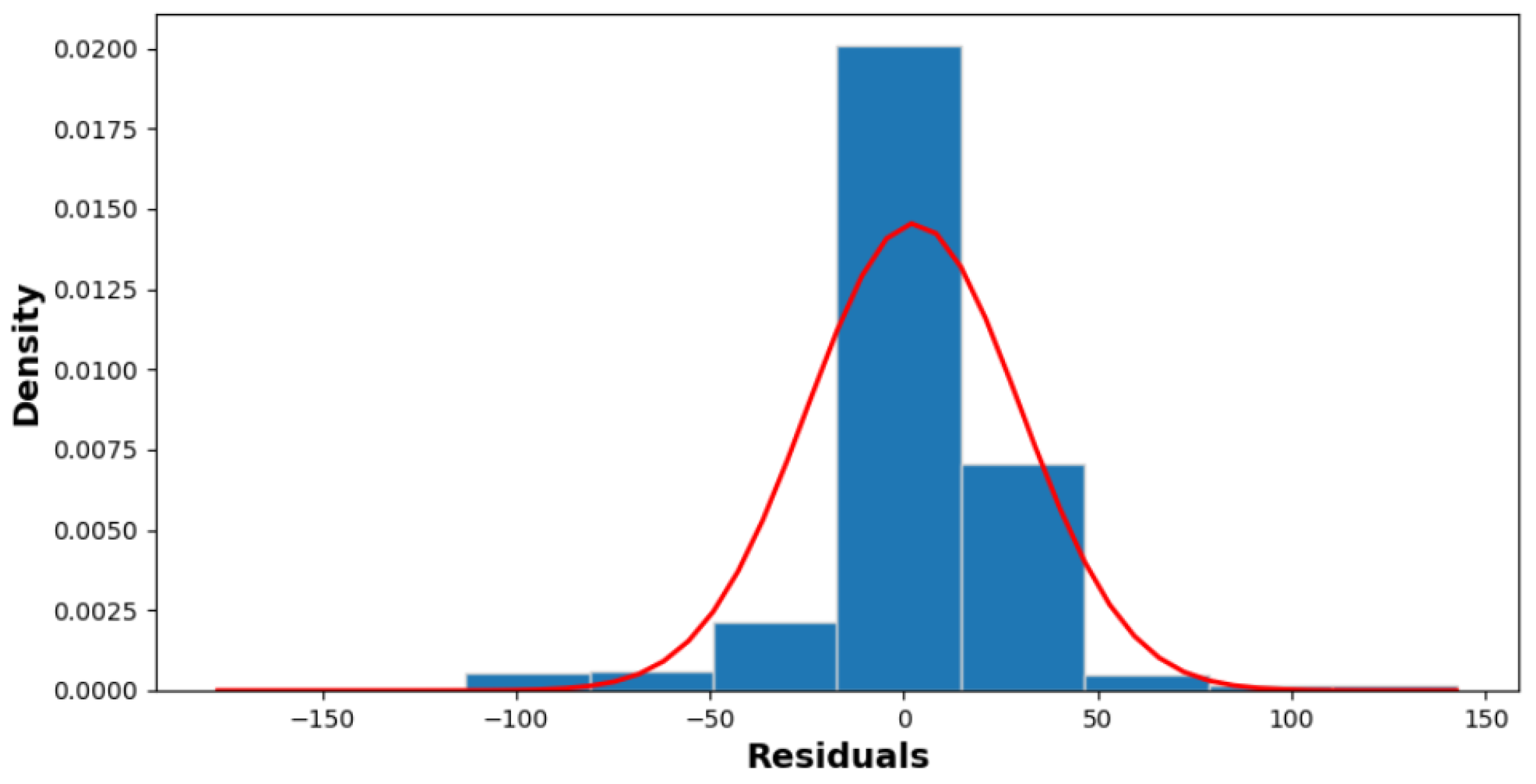
Figure 12 and
Figure 13 show the frequency distribution of residuals with an SD of 38.25 and a mean of 34 for sunny days and an SD of 27.42 and a mean of 17.13 for cloudy days, respectively.
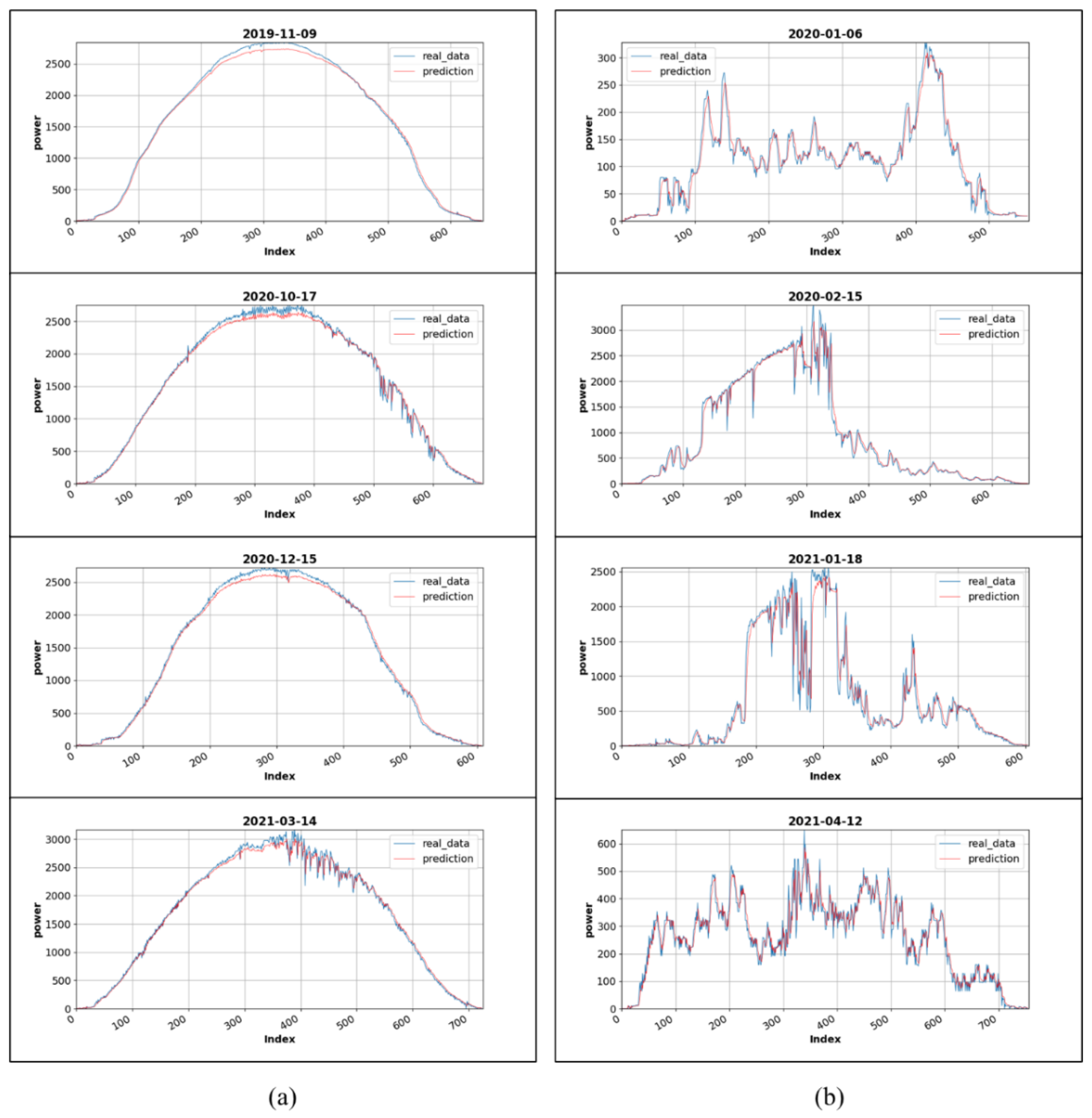
The advantage of the LSTM model is further highlighted when using unfavorable weather patterns.
Figure 14a,b show the qualitative evaluation results of various test data for the sunny and cloudy day data, respectively. The proposed algorithm adequately follows the trends in various power generation patterns for accurate forecasting. However, errors occur at peak points for the cloudy data with irregular patterns and large fluctuations. However, the algorithm is robust to abrupt changes in the patterns and fluctuation periods, thus reasonably following the trend for reliable forecasting. A qualitative evaluation confirms the high efficiency and improved performance of the proposed model in solving the PV power generation forecasting problem.
The power generation forecasting performance of the proposed model differs depending on the weather patterns and validation datasets. The characteristics of power generation fluctuation patterns are sufficiently captured by the CNN, while the LSTM finds long-term dependencies in the time-series input. In other words, the CNN-LSTM hybrid model may not produce the same result in an environment having different weather conditions. For example, the proposed model produced errors in the power generation peak points for the sunny day data but made accurate predictions by following the fluctuations pattern for the cloudy day data having abrupt changes.
5. Conclusions
A PV power generation forecasting model can improve prediction accuracy according to weather conditions and enhance the planning, operation, and stability of PV power systems. However, PV power generation forecasting can be challenging owing to intermittency in weather conditions. A statistical method for inferring dependency between past and short-term observed data is required to build an effective forecasting model that depends only on past data, excluding the solar radiation data highly correlated with power production.
This paper proposes a CNN-LSTM hybrid model for PV power generation forecasting. The proposed model overcomes the drawbacks of the individual models while preserving their advantages. Because training one LSTM model using different time-series data may affect network convergence, separate models were built according to weather conditions. Weather patterns were classified using CNN, and the LSTM model was applied to the classification results. The power generation patterns can clearly distinguish between sunny and cloudy days. The proposed forecasting model can sufficiently reflect the fluctuations in power generation for accurate forecasting. A qualitative evaluation confirmed that the forecasted power output signals react to fluctuations and adequately follow the actual power output signal trend.
Moreover, a quantitative evaluation demonstrated that the proposed model has RMSEs of 4.58 and 27.55, MAEs of 34.00 and 17.13, and MAPEs of 4.58 and 7.06 for sunny and cloudy day data, respectively. The residual distributions had an SD of 38.25 and a mean of 34.00 for sunny days and an SD of 27.42 and a mean of 17.13 for cloudy days, respectively, thus establishing the validity of the proposed model. The characteristics of collected data and power generation values may vary depending on the inverter manufacturer. Since the power generation capacity of a PV power plant system varies depending on installation scale and weather conditions, the model requires reconfiguration according to the power generation capacity. Future research should focus on methods for forecasting power generation by adaptively reflecting the power generation capacity of a PV power plant. This includes the application of optimization techniques that automatically perform model fitting according to the data accumulated in the system to improve the prediction accuracy; In addition, it is necessary to analyze factors affecting power generation efficiencies such as PV panel characteristics and solar radiation. Additionally, the forecasting results are expected to be used to understand the decrease in inverter efficiency over time. In cases where inverter power generation is less than the predicted generation, it will help determine whether the phenomenon is an efficiency decline due to the aging of the inverter.


