Smart Gas Network with Linepack Managing to Increase Biomethane Injection at the Distribution Level

Abstract

The current situation in Europe calls for the need of urgent measures to find sustainable alternatives to its outer dependence on natural gas. Biomethane injection into the existing gas infrastructure is a fundamental opportunity to be promoted that, however, causes increasing complexities in the management of natural gas grids. At the gas distribution level, the lack of a monitoring system and suitable software for the simulation, management, and verification of gas networks may act as barriers to a widespread diffusion of a biomethane production and injection chain. A transient fluid-dynamic model of the gas network is developed to perform estimations of the natural gas grid capacity in situations of production-consumption mismatch, taking into account the linepack as a gas buffer stock. The model is applied to the gas distribution network of a small urban-rural area. The aim is to assess the role of the linepack in determining the gas network receiving capacity and to test smart management of pressure set-points and injection flow rate to minimize biomethane curtailment. Results show that biomethane unacceptability can be reduced to 10% instead of 27% (obtained when following the DSOs state-of-the-art current procedures), thus highlighting the importance of the implementation of transient simulation software but also underlining the need for smarter control systems, actuators, and data management platforms for a transition to smart digital gas grids.

1. Introduction

The post-COVID-19 economic recovery, the subsequent supply crisis, and the outbreak of the Russian-Ukraine war all contributed to shaking the natural gas market with unpreceded consequences.

In early March 2022, the European Commission published the REPowerEU plan, to boost energy-saving measures, accelerate the promotion of clean energy forms, and overall, diversifying the European energy supply, with particular emphasis on the fast, complete, and permanent elimination of the dependence on Russian fossil fuels (particularly natural gas) [1]. This plan sets near-term actions (by 2022) and recasts the medium-term objectives of energy transition that were set a few months earlier within the Fit-for-55 program [2]. At this moment, renewable gases are seeing a historical growth of interest as the key element for an internal and non-fossil source of alternative gas with a particular focus on biomethane and hydrogen (green and blue). The 2030 biomethane production ambition has been forecast to be from 17 to 35 bcm, with 3.5 bcm to be placed on the market by the end of 2022.

Biomethane is defined as a fuel gas produced from biomass whose properties are comparable to the ones of natural gas (methane content > 95%) [3]. At present, it is mostly produced from the upgrading process of biogas produced by anaerobic digestion, consisting of the removal of contaminants and CO₂. The biogas from anaerobic digestion may contain between 25 ÷ 45–50% (molar based) of CO₂ [4,5] together with smaller amounts (traces) of contaminants such as hydrogen sulfide and ammonia that have to be cleaned out.

According to the European Biogas Association’s (EBA) Statistical Report 2021 [6], the number of installed plants in Europe multiplied by a factor of three between 2009 and 2016, with Germany, the UK, and Italy as the leading countries [7]. In Italy, a favorable feed-in tariff [8] has boosted small-scale (<1 MW_e) biogas power plants (mostly fed by energy crops [9]) since 2008, however, causing lagging in the development of the biomethane sector. As Italy lagged behind the goal of 10% of bio-fuels in the entire transport sector [10], from 2018 on, Italian policy has strongly committed to the promotion of biomethane production and injection into the natural gas infrastructure with the so-called “Biomethane Decree” [11].

Even though the biogas and biomethane sectors have always been strongly related, the last few years (from 2016 on) have recorded a much stronger build-up of the biomethane one, while the biogas sector was stagnating. The European biomethane production almost doubled, growing from 1.7 bcm in 2016 to 3 bcm in 2020 (with a strong increase between 2019 and 2021). Furthermore, in the biomethane sector, Germany leads with a yearly production of 1 bcm alone (data from EBA-GiE Biomethane Map 2020 [12]).

Biomethane plants may be considered a distributed and renewable source of natural gas. Its injection within the current infrastructure appears to be the straightforward and most sustainable practice to contribute to the greening of the gas sector. However, it is, to some extent, a revolutionary challenge for a sector whose state-of-the-art has been settled for years.

Technical regulation and standards at the European level have been developed thanks to the European Commission’s M/475 EN mandate [13] to CEN (European Committee for Standardization) on the standardization of biomethane injection criteria. It ended with the promulgation of the EN 16723 standard [14], directly implemented in Italy in the UNI/TR 11537:2016 technical standard [15]. Biomethane has to comply with the typical ranges of the fuel gases belonging to group H (higher heating value fuel gas). The national standards may differ from country to country with more stringent and specific limits (as in Italy) on compounds that are not usually present in natural gas but may appear in traces in the biomethane (e.g., ammonia, halogens, etc.). In case of non-compliance, any injection should be immediately stopped. In Germany, instead, the limits are different according to the type of gas network targeted by the injection [16]. Furthermore, to limit the impacts on the gas quality, the system operators are required to add LPG to increase the heating value, creating a gas with identical calorific properties as the one within the pipes, avoiding billing issues [17]. This is said to be an expensive part of biomethane upgrading and conditioning and it may be avoided by the adoption of suitable quality tracking systems by the system operators, as suggested in [18], to comply with accuracy requirements in billing processes. This is particularly impactful on the business of distribution system operators (DSOs), which used to operate local and lower-pressure portions of the infrastructure, which never had to deal with “unconventional” distributed sources of gas.

Not only did biomethane introduce the quality management challenge, but it also brought about the issues of the mismatch between production and consumption, especially on the lower pressure level of the infrastructure where a portion of the network serves local areas characterized by seasonal and limited consumptions. The aspect of limitations in biomethane receiving capacity is rarely taken into account in works assessing the biomethane injection potential at the regional or country level. In [19], this potential is evaluated considering only the presence of the natural gas network in the administrative subdivision being taken into account, without considering its actual receiving availability. When dealing with the downstream management of biomethane, a focus is on the choice of whether it is convenient to liquefy or inject it. In [20], a maximum connection cost threshold is given to justify the choice of grid injection, giving a further reason to investigate the field of low-pressure biomethane injection (to save both CAPEX and OPEX related to biomethane compression). As highlighted in [21], in which the authors proposed the revamping of a biogas power plant to a biomethane production facility, the availability of the natural gas infrastructure is not guaranteed at all and it has a strong impact on the economy of the options and thus on the final choice.

To the best of the authors’ knowledge, these bottlenecks in the biomethane value chain, caused by its integration with the existing gas infrastructure and the way gas networks are operated, have rarely been addressed in research even though it matters in the sector.

In Italy, at present (2022), the number of biomethane plants currently in operation is 27 but only four of them are already injecting at the distribution level [12] (pressure level less than 5 bar_g). Most gas DSO associations have published common guidelines to evaluate the acceptability of biomethane injection requests to guarantee the safe operation of the infrastructure [22], requiring that the biomethane injection point would never become the only gas-feeding point of the distribution network. Consequently, any innovative network management strategies, such as bi-directional gas reduction-and-metering stations and linepack buffering, are excluded.

Circumstances are different in other countries in Europe: it is worth underlining that definitions of distribution and transmission level are not univocally determined throughout the European gas system as well as the number of TSOs and DSOs managing the national systems, thus generating the premises to different approaches from one nation to another. For historical reasons, the number of Italian DSOs is almost 500, while other countries, such as Denmark and The Netherlands, have a much smaller number. In Denmark and Germany, the DSOs usually also run the higher-pressure portion of the network, insisting on greater areas. This is the reason why in [12], many biomethane plants are connected to distribution grids in states such as Denmark or France.

In Denmark, the limited capacity of distribution networks has been solved by adopting bi-directional reduction and metering stations returning the excess biomethane production to a higher pressure transmission level employing compression stations, thus inverting the usual gas flow on demand. According to the latest system plan by Energinet (the Danish TSO) [23], two gas return plants are already in operation and three more were in the planning phase as of 2022. Interestingly, as detailed in [24], for one of the already operating plants, an additional connection with a nearby distribution network, which used to be separated, was also planned, to distribute the biomethane throughout a greater consumption area. Such solutions are conceptually simple and technically feasible even though they add capital costs to the injection projects. However, they require a very good level of coordination between the different parties of the gas network value chain as well as updates to the regulatory framework. These institutional aspects may act as a barrier to the early implementation of these measures.

As for The Netherlands, the main transmission system operator (Gasunie) is taking part in Projectgroep Groen Gas, a working group of the Association of Energy Network Operators (Netbeheer Nederland) aimed at developing pilot projects to improve the biomethane acceptability within the current infrastructure. Among these, the case of bi-directional gas receiving stations is also addressed, together with more innovative projects aimed at generating a buffering storage capacity within the network itself. The latter appears to be one of the less impacting solutions in terms of capital expenditures, as it deals with the way the network is operated.

This paper aims to highlight the problem of the limited receiving capacity of a distribution network by showcasing a real case study of a gas distribution infrastructure. What is more, this work proposes a possible novel solution to limit the biomethane curtailment thanks to the network management possibilities offered by the simulation tool.

A transient gas network model is presented and applied to the network to simulate situations of exceeding production (and thus curtailed injection) to assess the criticalities (e.g., quantify the amount of curtailed biomethane).

The novelty of the proposed work is to test, through simulations, scenarios of short-term gas storage within the network linepack to avoid or minimize biomethane curtailment while operating the network within its technical limits. Even though the numerical results are case specific, they are remarking on and quantifying a limitation of the biomethane injection potential at the distribution level that is worth noting and investigating further in future works. The paper offers a methodology that could be applied to several other case studies for the sake of generalization. What is more, the authors’ confrontations with distribution system operators on the difficulties in managing the renewable gas inclusion within their infrastructure, confirmed by the trends in the biomethane plant grid connection, have motivated the study presented hereafter.

In the following, a suitable simulation tool is applied to a real distribution infrastructure to model strategies to enhance biomethane acceptability by managing the overall infrastructure buffering storage capacity.

2. Materials and Methods

The research presented in this paper is devoted to the simulation of distribution gas network assets when operated in a non-conventional way such as the injection of a fixed biomethane gas flow rate at a medium pressure tier. As this research aims to focus on the dynamics of the gas network when there is a mismatch between biomethane production and availability, a suitable fluid-dynamic model should be used.

A transient fluid-dynamic gas network model has been applied to a real distribution gas network, located in Northern Italy. The case study is the same used in [25], where the injection of a stream of raw biogas produced by a digester present in the area was simulated. In that case, a stationary and multi-component network model was used for the scope. In this case, the biogas is assumed to be upgraded to biomethane and to be injected into the existing infrastructure, thus a more detailed description of the time-dependent phenomena needs to be performed. The digester plant produces around 12,000 Sm³/d of biogas that is fed to an internal combustion engine that produces electrical power. The nominal size is 1 MW_e. As the composition is about 52% CH₄ and 48% CO₂ (molar-based), assuming a constant production rate and an ideal upgrading process, the possible biomethane production rate is equal to 6240 Sm³/d corresponding to 260 Sm³/h.

In the following section, the mathematical procedures for the formalization of the computational model are described. The model is written as MATLAB code and the simulations are performed in a MATLAB environment.

2.1. Gas Network Model Description

Fluid network models aim at solving the fluid-dynamic of the networks by determining the pressures of each junction of the infrastructure and the gas flows within each pipeline. A network is often represented as a topological object: an oriented graph, i.e., a mathematical representation of the connections between one junction and the others, thus defining the pipelines. In the mathematical taxonomy, the junctions are called nodes or vertices and the connections (with a direction specified) are the branches or edges. In the case of fluid networks, the edges are the pipelines.

When setting up a computational model, one of the most effective ways to represent a graph (i.e., the information about the structure of a network) is by an algebraic mean: the incidence matrix. This is defined as follows:

$$\begin{gathered} A={\left[a_{i,j}\right]}^{n\times b}, \\ {a}_{i,j}=\{\begin{array}{c}+1, \mathrm{edge} j \mathrm{is} \mathrm{outgoing} \mathrm{to} \mathrm{node} i\\ -1, \mathrm{edge} j \mathrm{is} \mathrm{incoming} \mathrm{from} \mathrm{node} i\\ 0, \mathrm{edge} j \mathrm{has} \mathrm{no} \mathrm{connections} \mathrm{with} \mathrm{node} i\end{array} \end{gathered}$$

For a network topology with n nodes and b edges (pipelines).

This algebraic structure is key for the solution of the fluid-dynamic problem for the whole network once the system of equations expressed for a single pipeline and node is linearized.

The fluid dynamics within a single pipe can be described by applying the following couple of conservation equations (here given in their 1D differential form):

Conservation of mass

$$\frac{\partial \rho }{\partial t}+\frac{\partial \left(\rho v\right)}{\partial x}=0$$

(1)

Conservation of momentum

$$\frac{\partial \left(\rho v\right)}{\partial t}+\frac{\partial \left(\rho v^2\right)}{\partial x}+\frac{\partial p}{\partial x}+\frac{f_d\rho v\left|v\right|}{2D}+\rho gsin\vartheta =0$$

(2)

where:

$\rho$: fluid density $\left(\mathrm{kg}/{\mathrm{m}}^3\right)$;

$v$: fluid velocity $\left(\mathrm{m}/\mathrm{s}\right)$;

$p$: fluid pressure $\left(\mathrm{Pa}\right)$;

$f_d$: friction factor $(-)$;

$D$: pipeline diameter $\left(\mathrm{m}\right)$;

The 1D simplification is justified by the fact that in pipelines the x-dimension, along the length, is often greater than the cross-sectional dimensions, thus allowing to consider the phenomena occurring on the cross-sectional plane as negligible. It is worth noting that the problem does not take into account temperature (allowing to avoid the third conservation equation—of energy). It is very common to assume the isothermicity of the problem given that most of the pipelines are typically buried at least one meter underground, thus making it possible to consider the surrounding temperature as constant and a thermal equilibrium between the gas, the pipeline, and the environment.

As additional simplifying assumptions, the kinetic and the gravitational terms (the second and the last terms in Equation (2)) can be neglected as commonly assumed in literature [26].

These assumptions are frequently adopted in the literature [26,27,28], in commercial software, and by distribution system operators (DSOs) for their ordinary business operations.

The fourth term in Equation (2) is the shear force term in which $f_d$ is the friction factor, which can be calculated using semi-empirical correlations as a function of the Reynolds number. In this specific case, the correlation used is the Cheng explicit formula [29].

In order to conclude the mathematical formulation of the problem, the equation of state for real gas has been considered:

Real gas law

$$\frac{p}{\rho }=Z\frac{R_0}{MM}T$$

(3)

where:

$Z$: compressibility factor $(-)$;

$R_0$: Universal Gas Constant $\left(\mathrm{J}/\mathrm{mol} \mathrm{K}\right)$;

$MM$: molar mass $\left(\mathrm{g}/\mathrm{mol}\right)$;

$T$: temperature $\left(\mathrm{K}\right)$;

The compressibility factor $Z$ is determined through the GERG 2008 equation of state [30], a multiparameter equation of state explicit in the Helmholtz free energy.

Having to apply the fluid-dynamic description given by the system of conservation equations to a problem where the knowns are pressures and gas flow rates, the equations are rewritten in terms of mass flow rates using the following definition:

$$\dot{m}=\rho vA$$

Thus, the conservation equations refer to more relevant quantities (with respect to the problem).

Conservation of mass

$$\frac{1}{c^2}\frac{\partial p}{\partial t}+\frac{1}{A}\frac{\partial \dot{m}}{\partial x}=0$$

(4)

Conservation of momentum

$$\frac{1}{A}\frac{\partial \dot{m}}{\partial t}+\frac{\partial p}{\partial x}+\frac{\lambda c^2}{2D{A}^{2}p}\dot{m}\left|\dot{m}\right|+\frac{gsin\alpha }{c^2}p=0$$

(5)

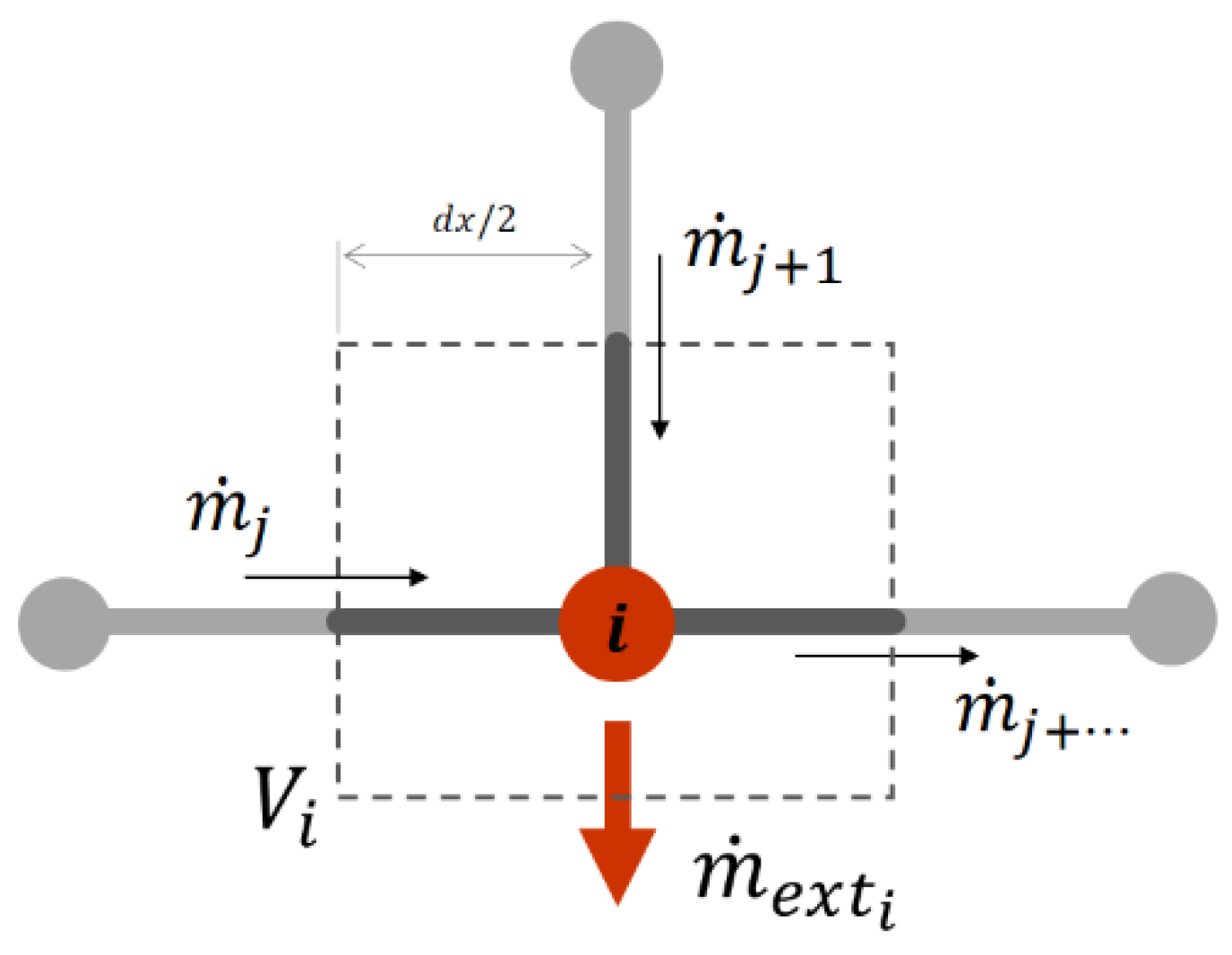
Now regarding the conservation of mass, the transformation of the differential equation to the algebraic equation, useful to be integrated into the complete network model, is given by its application on a control volume surrounding the generic i-th node (Figure 1)

After the integration of Equation (4) to the control volume, the time discretization by applying the backward Euler method, the generalization to the whole network of the nodal mass balance results in the following matrix form:

$$\mathit{\Phi }{\mathit{p}}^{t+1}+\mathit{A} {\dot{\mathit{m}}}^{t+1}+\mathit{I} {\dot{\mathit{m}}}_{\mathit{e}\mathit{x}\mathit{t}}{}^{t+1}=\mathit{\Phi }{\mathit{p}}^t$$

(6)

where $\mathit{I}$ is the identity matrix and $\mathit{\Phi }$ a diagonal matrix defined as follows:

$$\mathit{\Phi }={\left[{\varphi }_{i,i}\right]}^{n\times n},{\varphi }_{i,i}=\frac{V_i}{c_i^2 \Delta t}$$

(7)

Concerning the momentum Equation (5), its integration over an entire pipeline of length $l$ and its time discretization by applying the backward Euler method allows writing an equation for the pressure drops as follows:

$$\Delta P^{ t+1}=P_{in}^{t+1}-P_{out}^{t+1}=R_I·\left(\dot{m}{ }^{t+1}-\dot{m}{ }^t\right)+R_F·{\dot{m}}^{ t+1}\left|{\dot{m}}^{ t+1}\right|$$

(8)

where the substitution of a variable such as $P=p^2$ allows for a first attempt to linearize the problem, and the coefficients of the right represent two resistance coefficients representing the two physical phenomena contributing to the pressure variation along the pipeline:

$R_I=\frac{2 \overline{p^{t+1}} l}{A \Delta t}$;

$R_F=\frac{\lambda \overline{c^2} l}{D{A}^2}=\frac{16 \lambda \overline{c^2} l}{{\pi }^2{D}^5}$;

The first (subscript I) is the inertia contribution, which is proportional to the mass flow variation during the time interval $\Delta t$. The second is the fluid-dynamic friction (subscript F) within the pipe, quadratically proportional to the fluid velocity (and thus the mass flow).

As Equation (8) is a quadratic function of the mass flow, a linearization procedure is to be followed in order to build the full algebraic problem for the transient gas network solution. The linearization strategy has been presented in [31]. The pipeline-linearized equation for the whole network becomes:

$$A^t {\mathit{P}}^{t+1 \left(k+1\right)}-R {\dot{\mathit{m}}}^{t+1 \left(k+1\right)}=-R_F\left(\left| {\dot{\mathit{m}}}^{t+1 \left(k\right)}\right| \circ {\dot{\mathit{m}}}^{t+1 \left(k\right)}\right)-R_I {\dot{\mathit{m}}}^{t \left(k\right)}$$

(9)

where $\mathbf{R}$, ${\mathbf{R}}_{\mathbf{F}},$ and ${\mathbf{R}}_{\mathbf{I}}$ are the (b × b) square diagonal matrices whose general elements (j, j) are the coefficients of Equation (8) (and their combinations according to the linearization procedure) corresponding to the j-th pipe. Of note is that the operator $\circ$ stands for the element-wise product.

In order to refer to the vector of nodal pressures $\mathit{p}$, the whole equation has to be divided by $\left(p_{in}+p_{out}\right)$ for each pipeline j.

It is worth noting that the right-hand side of Equation (9) is the known term of the equation, and it is composed of the “old” mass flow ${\dot{\mathit{m}}}^{t \left(k\right)}$, belonging to the previous timestep, and of the “tentative new” mass flow ${\dot{\mathit{m}}}^{t+1 \left(k\right)}$, originated from the iterative procedure for the solution of the linearized version of the pipeline equation.

The algebraic system formed by Equations (9) and (6) accounts for b + n equations with b + n + n unknowns, these being:

• b mass flow rates for each pipe;
• n pressures for each node;
• n mass flow rates exchanged with the external environment.

An additional set of n equations needs to be provided. This set of equations is in fact representative of the n boundaries conditions, which needs to be specified at any nodes of the network.

A general linear equation can be written to include all the possible cases of nodal control modes, which acts as boundary condition assignment in terms of mathematical formalization of the problem. The equation, in its scalar form results as:

$$k_{p,i }{p}_i^{t+1}+k_{m,i }{\dot{m}}_i{}^{t+1}={\beta }_i^{t+1}$$

(10)

where the coefficients $k_{p,i }$ and $k_{m,i }$ assume either value 0 or 1 according to the control mode of the i-th node, and ${\beta }_i^{t+1}$ is the set point value of pressure or exchanged mass flow for the time step $t+1$.

This equation is valid for the n node, thus providing the set of equations that were missing.

Table 1. Summary table for nodal possible control modes and corresponding boundary equations.

Control Mode	Equation	Coefficients
pressure	$p_i\left(t\right)=p_{set}{}_i\left(t\right)$	$k_{p,i }=1, k_{m,i }=0, {\beta }_i=p_{set}{}_i$
mass flow	${\dot{m}}_{ex{t}_i}\left(t\right)={\dot{m}}_{se{t}_i}\left(t\right)$	$k_{p,i }=0, k_{m,i }=1, {\beta }_i={\dot{m}}_{se{t}_i}$
junction/no flow	${\dot{m}}_{ex{t}_i}\left(t\right)=0$	$k_{p,i }=0, k_{m,i }=1, {\beta }_i=0$

sums up the possible nodal control mode and the corresponding boundary equations that originate.

The fluid-dynamic model of a complete gas network under non-steady state assumptions is given in the form of a linear matrix equation, which is the result of the composition of the pipeline equation, Equation (9), and the nodal balance equation, Equation (6), together with the matrix version of Equation (10), which includes all the boundary conditions of the problem. The complete problem takes the following form:

$$\left( \begin{array}{ccc}\Phi & A& I\\ {A^{\prime }}_g^t& -R^{\prime }& 0\\ K_p& 0& K_m\end{array}\right)\left(\begin{array}{c}{\mathit{p}}^{t+1}\\ {\dot{\mathit{m}}}^{t+1}\\ {\dot{\mathit{m}}}_{\mathit{e}\mathit{x}\mathit{t}}^{t+1}\end{array}\right)=\left(\begin{array}{c}\mathit{\varphi } {\mathit{p}}^t\\ \mathit{r}\\ \mathit{\beta }\end{array}\right)$$

(11)

Knowing the state of the network at time step $t$, it is possible to compute the nodal pressures, pipeline mass flows, and the nodal mass flows injected/withdrawn at time step $t+1$, according to the set points at the boundaries, thus defining the subsequent state of the network. Repeating this operation for the whole simulation interval, the evolution in time of the gas network is simulated. It is worth noting that, even though the complete problem in Equation (11) has the form of an algebraic system of equations, the computation of the gas network state at time step $t+1$ is performed by means of an iterative procedure. The need for an iterative procedure originates from the linearization approach to simplify the non-linearity of the momentum equation. The coefficients of matrices $\mathit{\Phi }$, ${{\mathit{A}}^{\prime }}_{\mathit{g}}^{\mathit{t}}$, and ${\mathit{R}}^{\prime }$ all depend on the unknown pressures and the mass flows. It is thus necessary to check for the approximation errors through the evaluation of the residuals: the solution of the ($k+1$)-th iteration ${\left( p, \dot{ m,} {\dot{m}}_{ext} \right)}^{t+1 \left(k+1\right)}$ is substituted within the continuity equation and the momentum equation in order to evaluate the residuals of the mass and momentum equations ($\mathit{R}\mathit{e}{\mathit{s}}_{\mathit{c}\mathit{o}\mathit{n}\mathit{t}}$ and $\mathit{R}\mathit{e}{\mathit{s}}_{\mathit{m}\mathit{o}\mathit{m}}$).

One of the most common convergence criteria refers to the Euclidean norm of the residual vectors. Most stringently, one can refer to the maximum value among the elements of the vectors. The possible set tolerance is (10⁻³ ÷ 10⁻⁸).

2.2. Conditional Boundary Conditions

When gas networks are operated at ordinary operating conditions, the gas pressure at the inlet gas nodes is fixed and kept constant by means of a properly set pressure regulator. If the downstream pressure becomes higher than the pressure set point, the gas flow must be stopped. According to the computational model structure, the boundary conditions given at each node can alternatively either be to control mass flow (entering or exiting) or to control pressure. Thus, when gas pressure becomes higher than the set-point value given at the pressure-controlled node (usually the inlet), an inversion of the gas flow happens at this node. This is in fact the only possible solution to comply with the pressure constraint of the boundary condition. For the sake of this work, this is considered to be a non-realistic situation. The boundary conditions setting phase needs to be conditional according to the network status. When the pressure field is such that it implies an inversion at the city gate, a shift from pressure control to mass flow control needs to happen, and specifically the mass flow rate has to be set to zero.

Thus, the following conditional boundary condition at the city-gate reduction station is given:

$$\{\begin{array}{c}p\left(i,t\right)=p_{set}{}_i\left(t\right) if p_{set}{}_i\left(t\right)>p \left(i+1, t\right)\\ u\\ {\dot{m}}_{ext}\left(i,t\right)=0 if p_{set}{}_i\left(t\right)\le p \left(i+1, t\right)\end{array} \forall t$$

(12)

where $i$ is the city-gate reduction station node and $i+1$ is the adjacent node.

Referring to the boundary condition equation (Equation (10)), the coefficients will be modified as follows:

$$\{\begin{array}{c}{k}_{p,i}=1 , k_{m,i}=0, {\beta }_i=p_{set}{}_i\left(t\right) if p_{set}{}_i\left(t\right)>p \left(i+1, t\right)\\ u\\ k_{p,i}=0, k_{m,i}=1, {\beta }_i=0 if p_{set}{}_i\left(t\right)\le p \left(i+1, t\right)\end{array}$$

(13)

2.3. Case Study Description

The case study refers to a small municipality composed of two urban agglomerations, three industrial areas, and rural areas surrounding these major consumption centers. It covers a surface of 29 km² with a population of approximately 6500 inhabitants and 3262 active gas meters, only 6% of which are classified as industrial users. The annual gas consumption of the area is equal to 8.25 MSm³. Despite the proportions of the gas meters, the industrial users generate 59% of the annual gas consumption of the whole area while the remaining 41% is generated by the residential and tertiary sectors. The gas network modelled in this work corresponds to the real network asset of the case study. 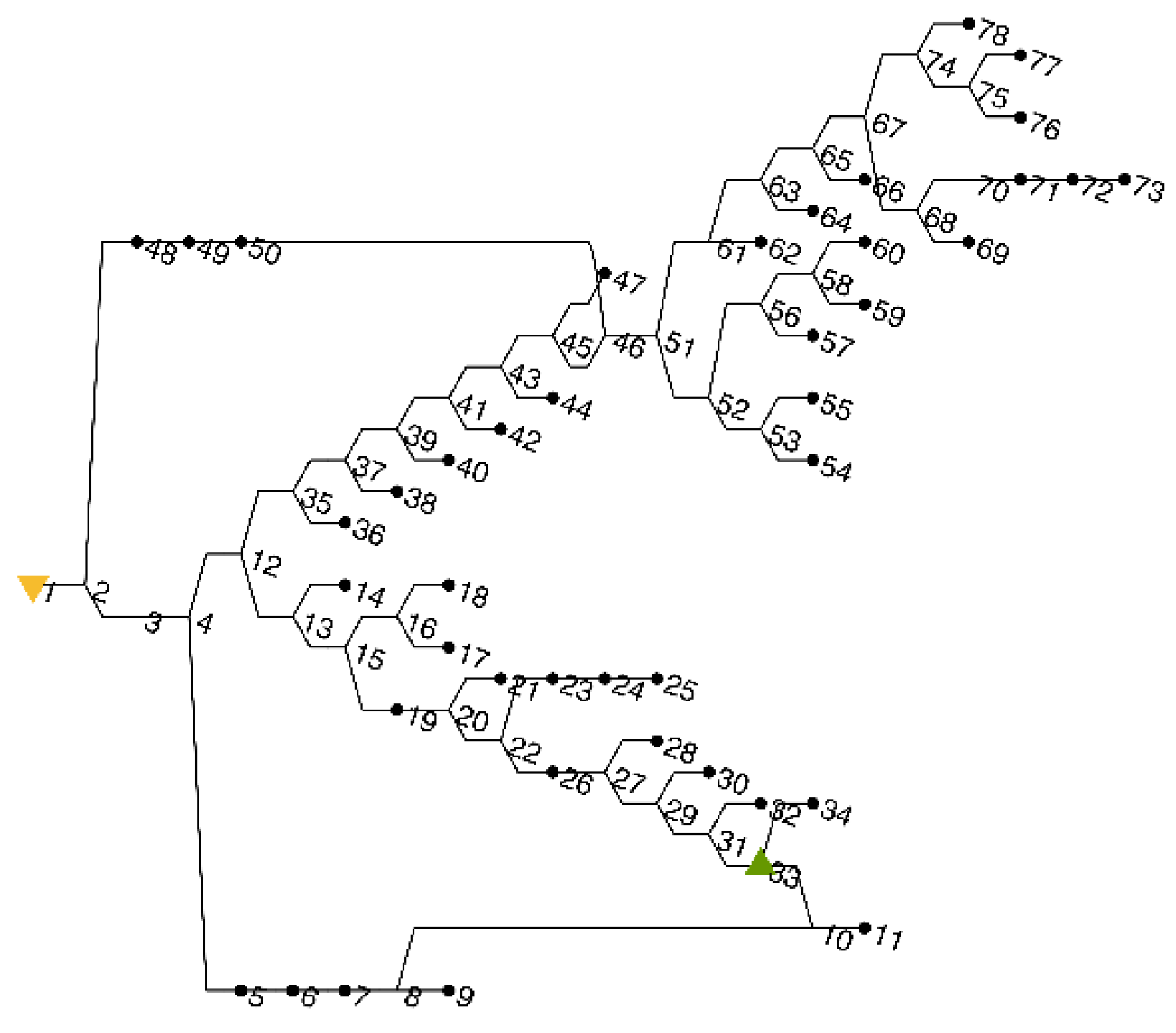The authors have already used this infrastructure for previous studies, thus more details on the technical feature or the gas consumption profiling are presented in [25]. A simplified and distorted scheme of the network topology is given in Figure 2. Only the medium pressure tier, corresponding to gas pressure in the range [5–1.5] bar_g, will be addressed in this study. The fossil natural gas inlet node is highlighted with a yellow triangle while the green triangle indicates the location of the biomethane injection. Bullet-shaped nodes represent a user or a cluster of users (i.e., a gas exit point).

Concerning gas consumption and profiles, the only real available data consist of yearly basis gas consumption. For the sake of this case study, a higher time resolution would be desirable (at least 1 h). While the procedure of distributing the yearly gas consumption into a daily profile is regulated by the Italian energy authority through resolution 229/2012 [32], some assumptions have been made to generate infra-daily profiles.

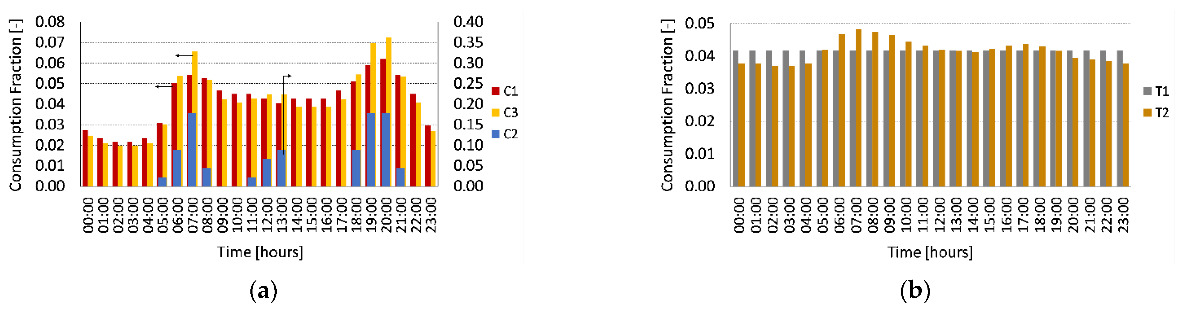
A set of daily gas consumption profiles have been proposed and reported in Figure 3. The profiles are the hourly fraction of the total daily consumption. The hourly profile of each user can be obtained by multiplying the daily consumption with the profile corresponding to the user category.

The different colored bars refer to the different categories of gas usage, following the definitions given in resolution 229/2012 [32]. There are five relevant to the case study and they are listed with a short explanation in

Table 2. Gas usage categories [32].

Code	Description	Seasonality
C1	Space heating	yes
C2	Cooking and/or DHW	no
C3	Space heating + cooking and/or DHW	yes
T1	Technological use	no
T2	Technological + space heating	yes

.

It is worth noting that the indication of seasonality is relevant for the infra-annual profiling starting from the aggregated yearly values. In fact, all seasonal-dependent categories undergo a major change in the daily gas consumption when shifting from the space heating season to the warmer season causing the typical difference between the overall network winter consumption and summer consumption. Besides this, to complete the overview of the final users’ taxonomy, for each of these gas usage categories, three additional withdrawal classes are assigned, depending on the weekly frequency of the use of gas as described in

Table 3. Class of withdrawal [32].

Code	Withdrawal Days
1	7 days per week
2	6 days per week (excluding Sundays and national holidays)
3	5 days per week (excluding Saturdays, Sundays, and national holidays)

.

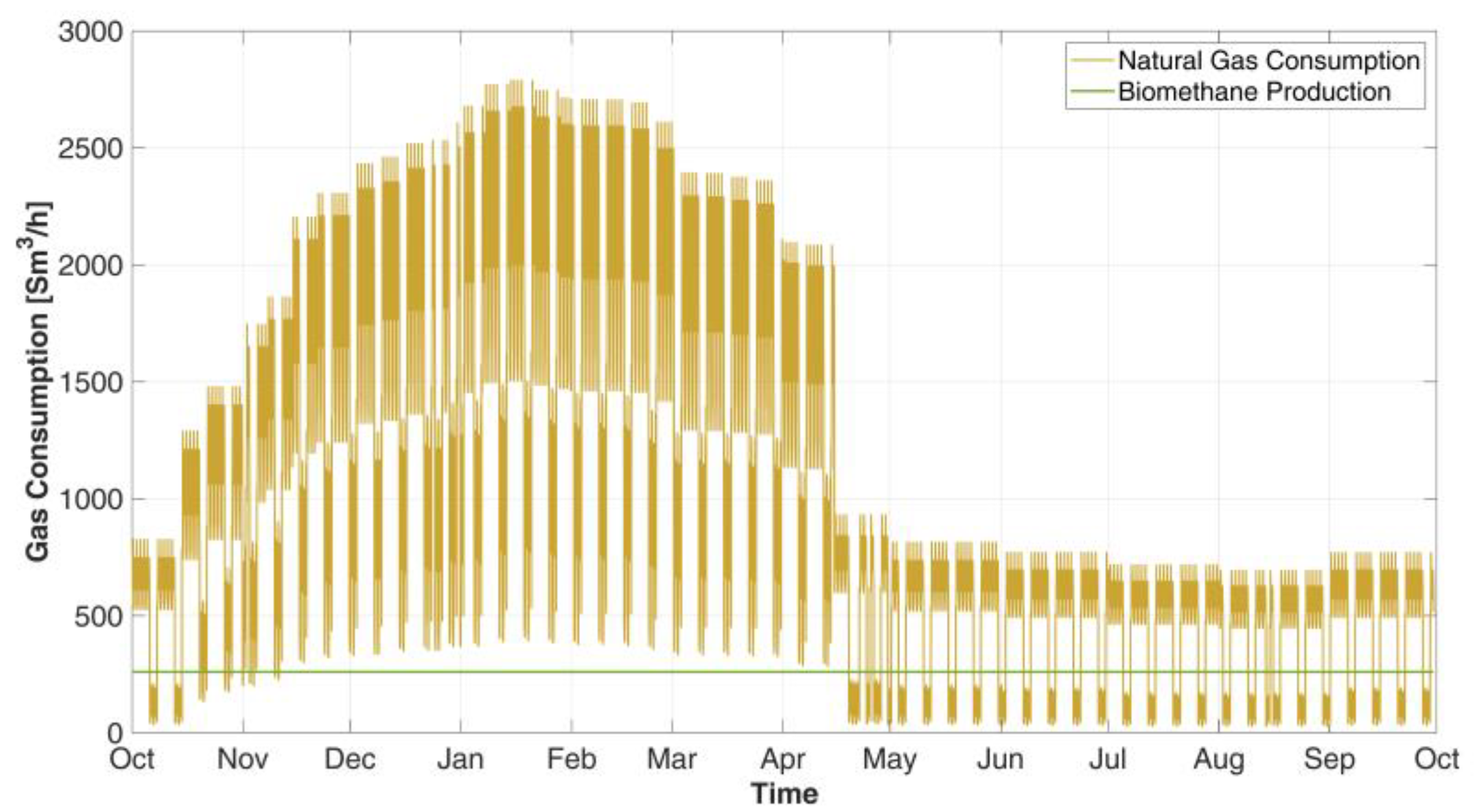
The case study presented here is built around the testing of the scenario of biomethane injection. The rural area is already equipped with a biogas power plant of 1 MW_e, thus an assumption is made consisting of repurposing the existing plant for biomethane production. As a result of the repurposing, the biomethane flow rate availability has been estimated to be around 260 Sm³/h, as previously mentioned. The choice of the injection node has been done by considering the shortest possible path.

2.4. Methodology

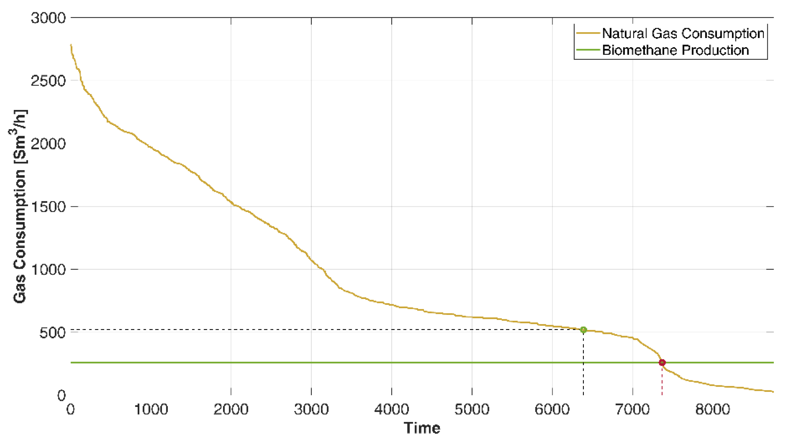
As the overall gas consumption of a distribution network usually has a remarkable variation from the winter season to the summer, while biogas and biomethane production is more or less constant in the business-as-usual scenario, issues of mismatches between production and consumption may arise, especially if the distribution networks serve smaller communities.

The case of gas accumulation within the linepack of the infrastructure is thus considered and the measures for the improvement of linepack storage are tested in this work.

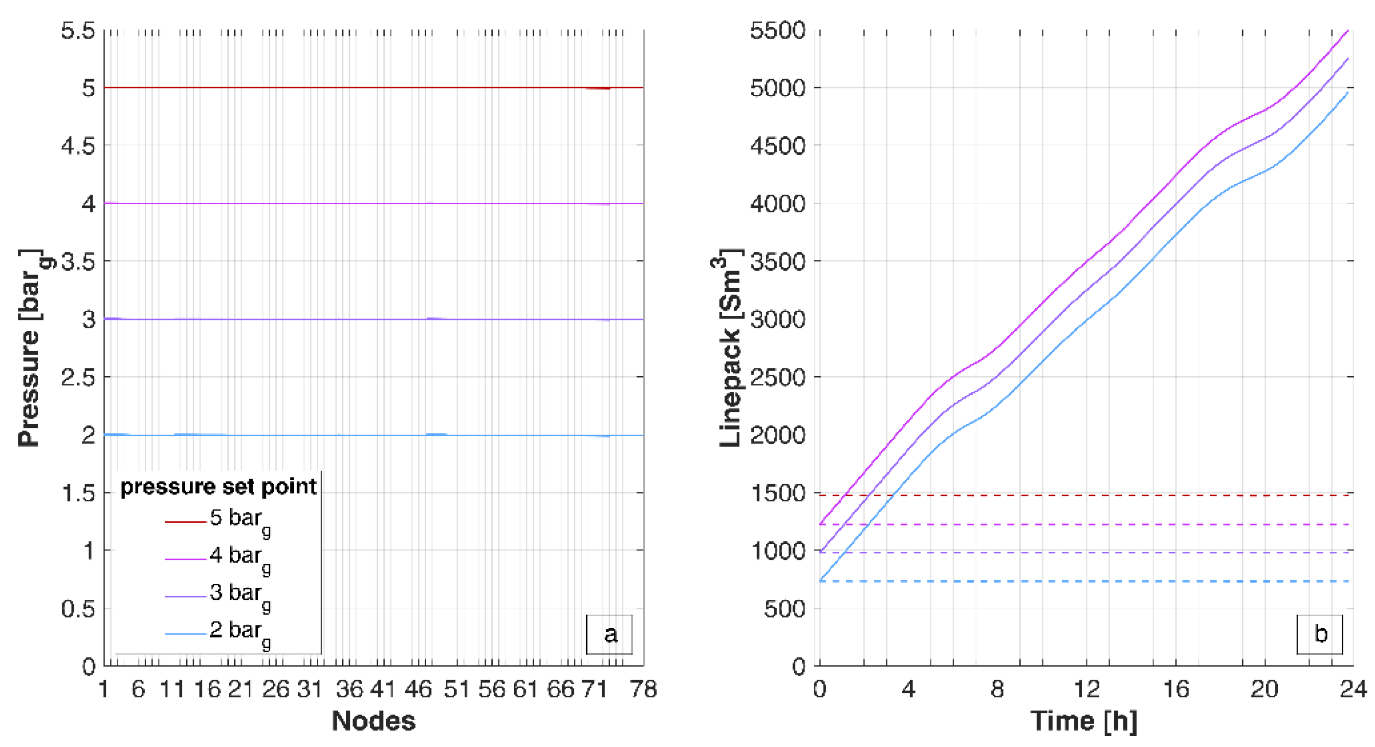
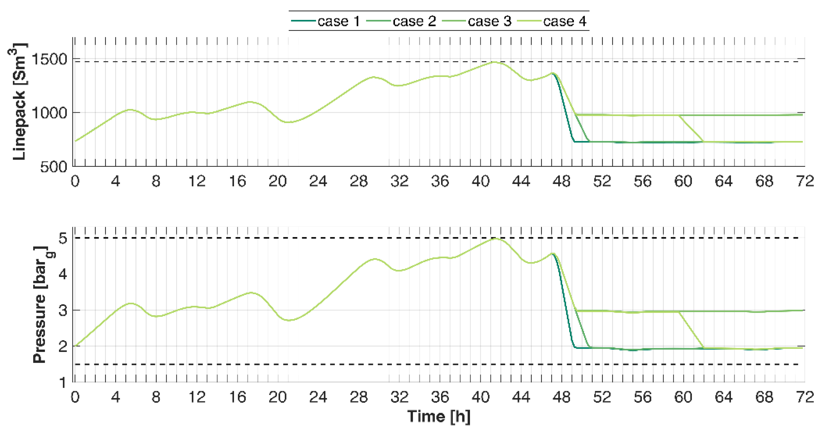
At first, the pressure level set point is lowered by 1-bar steps, in order to unlock linepack capacity, considering as the maximum acceptable linepack value, the one generated by a network that is set to 5 bar_g as the operating pressure.

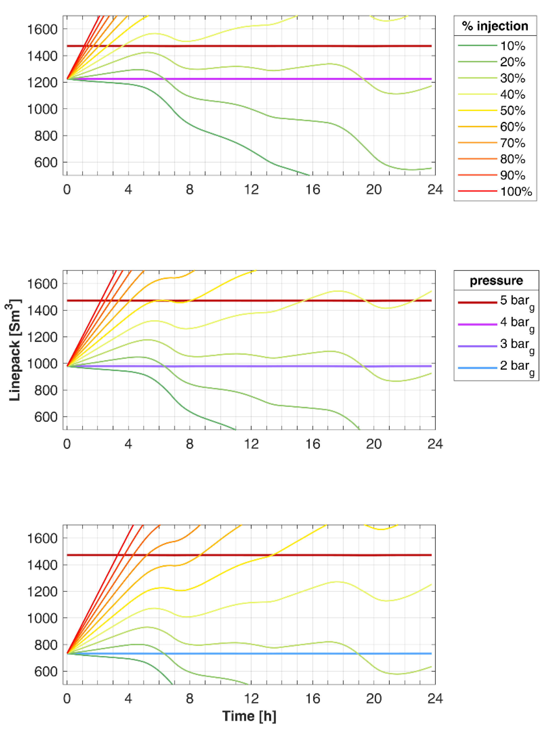
For each case, the hydraulic verification of the network is performed for both the non-injection and the injection cases. The first verification is needed to guarantee that nodal pressure does not drop below a minimum value. The second verification checks the gas accumulation curve and the network saturation time.

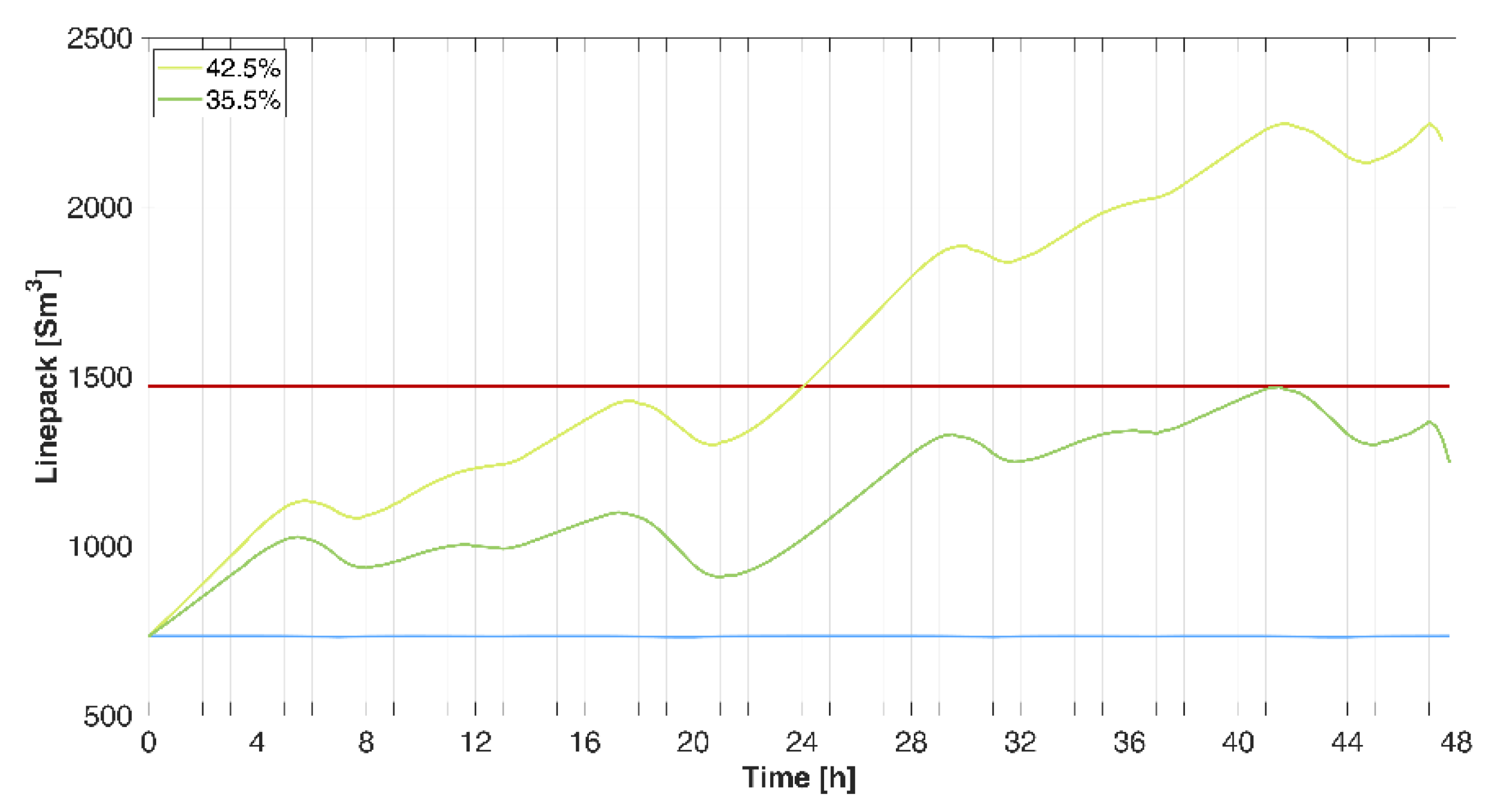
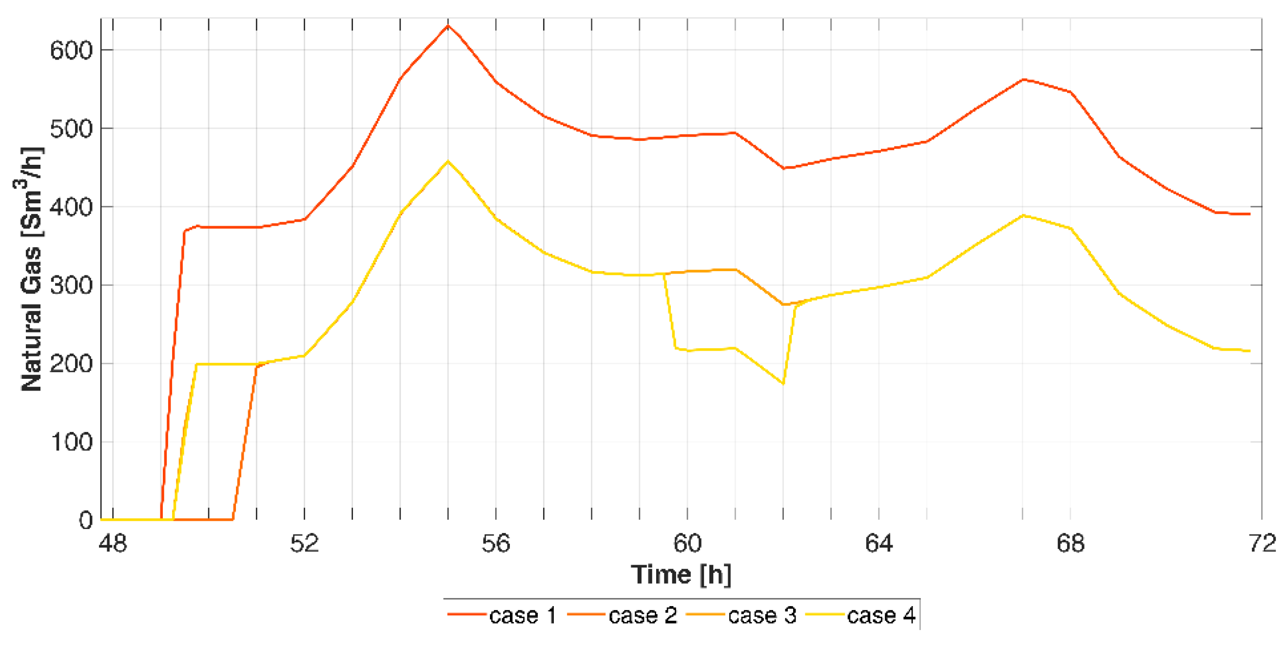
In the second phase, a reduction of the injected biomethane is imposed to modify the gas accumulation curve in order to determine the proper balance among biomethane injection, gas consumption, and linepack accumulation, which guarantees that the network operates within its limits.

The injection scenario determined through this analysis is then verified on a sequence of critical summer days, in which modifications of the pressure set points are also simulated to set up the case of modulating inlet pressures.

3. Results

3.1. Preliminary Production-Consumption Analysis

The acceptability of the biomethane injection flow rate, calculated to be about 260 Sm³/h, is to be verified with the model, under different gas network working conditions.

In Figure 4, the year-round total gas consumption on an hourly base, as obtained by applying the procedure in the previous section, is compared to the hourly biomethane production.

As can be seen, biomethane production is not always acceptable within the infrastructure. In fact, the biomethane production is completely absorbed by the overall gas consumption during most of the heating season (which, according to the location of the area, officially starts on 15 October and ends on 14 April), while it always exceeds the consumption during the weekends of the non-heating season.

The variation of consumption between the heating and non-heating seasons has a remarkable impact on the gas pressure distribution throughout the network. The fluid-dynamic gas network model is used to simulate two extreme gas consumption circumstances: maximum winter case consumption and minimum summer day consumption, both in the scenario of no injection of biomethane. Both gas pressure profiles have been overlapped in Figure 5.

In the summer case, the maximum overall pressure drop is in the order of millibars, while in the winter case this value is slightly more than 1 bar.

Consequently, in the summertime case, the pressure of the network can be considered equal to 5 bar_g throughout the network, thus implying that the linepack of the gas network is always at its limit. This means that the gas network is not able to accept any additional inlet gas flow that is not counterbalanced by suitable consumption. That is to say that the storage capacity of the network is already at its limit. On the other hand, it is possible to infer that for the summer case, the pressure set point at 5 bar_g is much higher than the needs.

3.2. Unlocking of the Linepack Storage by Pressure Modulation

The fact that the pressure is much higher than needed may lead to questioning the opportunity to keep this set point this high or whether it is possible (and even convenient) to lower the pressure set point when consumptions are considerably lower, thus decreasing the overall operating condition of the network. Figure 6a shows the nodal pressure sequence referring to the maximum consumption hour of the summer day considered before, under different pressure set points, for the case of no distributed injection. Correspondingly, in Figure 6b the dashed lines represent the linepack under the non-injection case for the different test pressures.

From this analysis, it is possible to draw the conclusion, on the one hand, that even at very low-pressure set points, the network can guarantee proper operating conditions. On the other hand, lowering the pressure set point allows for the unlocking of a linepack storage capacity. The difference between the amount of linepack when the network is operated at 5 bar_g (red dashed line) and the linepack at lower pressure indicates the hourly amount of gas that is virtually storable within the geometrical volume of the network while keeping the pressure level below the maximum acceptable pressure. Figure 6b shows that, under these working conditions, the linepack decrease is linear with the decrease of the operating pressure of the network. The rate of linepack decrease for each bar is 33%, corresponding to an additional storage capacity of about 245 Sm³ each hour. This allows the network to be more flexible in accepting imbalances between inflows and outflows and thanks to the accumulation of gas within the pipelines.

The gas accumulation function is depicted in Figure 6b by the solid lines. They are obtained from the time integral of the inlet-outlet mass flow balance of the whole network as follows:

$$LP\left(t\right)=L{P}_0+{{\displaystyle \int }}_{t=0}^{t_{end}}\Delta \dot{M}\left(t\right) dt$$

(14)

where:

$$L{P}_0={{\displaystyle \sum }_{j=1}^{\# pipes}{\frac{A}{c^2} {{\displaystyle \int }}_{x=0}^{x=l}p dx |}_j|}_{t=0}={{\displaystyle \sum }_{j=1}^{\# pipes}\frac{{\overline{p}}_j}{c_j^2} V_{geom}{}_j |}_{t=0}$$

is the initial value of the total network linepack, obtained as a summation of all the single j-th pipeline linepacks. It depends on the choice of the pressure set point of the network.

$$\Delta \dot{M}\left(t\right)={{\displaystyle \sum }_{i=1}^{\# nodes}-{\dot{m}}_{ex{t}_i}\left(t\right) |}_{\forall t}$$

is the gas accumulation term, resulting from the balance between the inlet and outlet gas flows. According to the convention of signs considered in the model structure, a minus sign is needed to consider the inlet flows as positive, in order to have an accumulation. Linepack and accumulation terms may be expressed in standard cubic meters rather than kilograms by considering the density at standard reference conditions (here: T = 15 °C and p = 1 atm).

From Figure 6b, it is possible to measure the increase in the storage capacity of the network as a consequence of the lowering of the pressure set point. The intersection between the solid lines and the dashed red line, which corresponds to the maximum acceptable linepack, indicates the time when the network is saturated by the constant injection of the whole production of the biomethane. Results are summarized in

Table 4. Network accumulation capacity of biomethane generated with the decreasing of the pressure set point for each pressure level analyzed and related saturation time of the network under the case of complete injection of biomethane.

Pressure Set Point	4 barg	3 barg	2 barg
Saturation time	1 h 7′	2 h 12′	3 h 18′
Accumulation capacity	247 Sm3/h	493.3 Sm3/h	738.6 Sm3/h

, where the network saturation times are given for the addressed cases. The lower the starting pressure set point, the higher the accumulation capacity of the network, and the longer the time before the network is saturated.

It is possible to conclude that, concerning this case study, each bar of decrease allows the network to gain slightly more than 1 h of line storability, thus providing flexibility to the system as well as improving renewable gas acceptability.

Of course, this result is specific to the case study addressed: it depends on the total geometric volume of the network and the balance between gas consumption and biomethane injection flow rate. From this first investigation into the exploitation of linepack gas storage, it has been observed that operating the network at lower pressure is useful to unlock the linepack storage potential. However, this newly created flexibility may not be enough to counterbalance the mismatch between production and consumption. It can only provide some lagging time before the injection cut-off happens. To avoid this circumstance, a reduction of the biomethane inlet flow rate is to be imposed.

3.3. Biomethane Injection Partialization

The effects of the reduction of the biomethane injection on the gas accumulation function are depicted in Figure 7, for each of the pressure reduction scenarios discussed before. Each graph refers to one inlet pressure set point (p_set = 4 ÷ 2 bar_g from the top to the bottom), which defines the linepack for the non-injection case and gives the initial linepack condition $L{P}_0$ for the calculation of the accumulation trajectories under different injection reduction scenarios. These scenarios consist of a progressive reduction of 10% of the inflows of biomethane, thus producing ten possible linepack evolutions, under the assumption that the city-gate entry point is not exchanging any mass flow. The analysis depicted in the figure, presents the complete set of possibilities of biomethane acceptability improvement by the combination of the pressure decrement and injection limitations, to avoid the complete cutting-off solution.

From the figure, it is clear that in the case of a network at 4 bar_g (upper plot), the reduction of the biomethane injection to 40% of the biomethane production is still not sufficient to avoid overpressures. It is necessary to drop the injection down to 31.8%. Turning the network to 3 bar_g (middle plot) allows the injection of 37.1% of the biomethane production. Lastly, dropping the network set point to 2 bar_g (lower plot) grants the acceptability to 42.5% of the produced biomethane (the 40% line lies completely within the acceptability range of linepack volumes). Thus, in the context of limiting the biomethane injection, lowering the pressure set point allows for a higher fraction of the production allowable in injection, with an almost linear increase between 4 and 2 bar_g gaining about +5.3% per bar_g in the fraction of injectable biomethane.

As a side comment, it can be noted that at percentages of biomethane injection up to 30%, the linepack evolution drops down the linepack level corresponding to the non-injection scenario at the desired pressure set point. This is possible under the assumption of the deactivation of the city-gate reduction station. In this situation, biomethane is the only gas source of the network and, at too low an injection percentage, it starts to become insufficient, thus emptying the linepack of the network. In reality, this would not be the case since the city gate would provide fossil natural gas as fast as the pressure of the network drops lower than its set point.

It is worth saying that this acceptability scenario is tailored for a one-day-long low-consumption network status. Results are different if the consumption-production mismatch lasts longer. This is the common situation for a summer weekend when industrial gas usage is lower and heating systems are turned off. Predictions of the duration of the possible mismatch are important in order to set up the most profitable strategy. In fact, in the context of biomethane injection reduction, what was concluded by the analysis of Figure 7 may lead to over-accumulation during the next day. Specifically, considering the case of a 2 bar_g set point and the maximum possible injection rate of 42.5%, it can be noted that the evolution of the linepack is increasing and already at its maximum. A repetition of a consumption pattern similar to the one of the day before, with no modification on the injection side, would soon lead to overcoming the linepack limit, as shown in Figure 8. It is then necessary to further decrease the acceptable biomethane injection.

Considering the whole duration of the critical operating condition of the network (i.e., the two days of a summer weekend), it results that, in the case of the pressure set point already lowered to the minimum, the biomethane injection has to be limited to 35.5% of the total production. In this way, the storage potential of the linepack, unlocked by the modulating pressure measure, is fully exploited without any violation of the operating conditions.

4. Discussion

Gas distribution networks are usually managed passively in order that the inward gas flow rate at the primary reduction station is the result of the balancing of the overall gas demand of the area; whenever the production exceeds the overall consumption, the biomethane cannot be accepted in injection and it is cut-off from the grid. This circumstance, otherwise, would imply the accumulation of gas within the pipeline and it cannot be handled by most DSOs at present (it is also excluded by the guidelines [22]).

Under this business-as-usual approach, only a fraction of the yearly produced biomethane can be accepted in the network. This value can be retrieved from the following duration curves (Figure 9), which display the allowable biomethane under two different assumptions.

The red dot and dashed line define the maximum number of hours of biomethane acceptability under the least stringent constraint according to which the biomethane is always accepted provided that consumptions are higher or equal to the production. However, most DSOs may want to keep a safety margin that consists of always keeping the traditional city-gate reduction station in operation, avoiding the whole network that would be fed exclusively by the biomethane injection [22]. This has a twofold purpose: on the one hand, it is a preventive measure in case of unexpected lower consumption rates; on the other, it prevents possible gas shortages in case the biomethane injection is stopped because of gas quality deviations or unplanned stops of production.

A good rule of thumb is to consider that the traditional reduction station should provide at least half of the total gas consumption. This may result in a reduction of the accepted injection rate or, as in the case of Figure 9, the reduction of the timespan of acceptability of the whole production (green dot and black dashed lines).

By implementing linepack management by only reducing the set-point pressure, the additional amount of injectable biomethane is negligible; as shown by results, managed in this way the network could only act as a few-hours buffer. Considering the case of both pressure management and injection flow rate reduction, more satisfactory results are obtained. As the most frequent situation is a production-consumption mismatch lasting for two days, this scenario is the one to be considered for comparison. By both lowering the pressure set-point at the minimum possible level (i.e., 2 bar_g) and allowing only 35.5% of biomethane production, roughly 128.000 Sm³ of biomethane can be injected additionally, which corresponds to about an additional 483.8 equivalent hours of full injection, thus increasing the biomethane injection allowance by +5.7% with respect to the curtailment case with “loose” criteria. This allows for obtaining 89.9% of the yearly injection factor. The obtained results are summarized in the following table (

Table 5. Results of the preliminary production-consumption analysis in the business-as-usual injection scenario under two different curtailment assumptions.

Curtailment Criteria	Yearly Injection (MSm3)	# Hours	%	% of Biomethane Curtailment
strict	1.66	6389	72.9	27.1
loose	1.91	7369	84.1	15.9
with pressure and injection management	2.05	7852.8 *	89.6	10.4

* Equivalent hours, i.e., number of hours if the biomethane injection would always be constant.

).

To complete the discussion around the increase of biomethane injection, it is necessary to underline that there is still a non-negligible fraction of biomethane that is not injectable, even in the most promising case. For full recovery of the biomethane in the scenario with pressure and injection management, the needed storage capacity is 7740 Sm³ to overcome two days of production-consumption mismatch.

The measure taken thus far to maximize biomethane injection should, lastly, be verified in the transition towards a higher consumption day, in which the linepack storage is not needed anymore because consumptions are greater than biomethane production. With higher consumptions on the one hand and a low-pressure set point on the other, pressure drops may increase and nodal pressure should be verified. Furthermore, the impact of restoring the biomethane injection to 100% of the production should also be evaluated.

In Figure 10, different scenarios for the transition to the third day (a weekday) are considered from the point of view of the variation of the linepack and the nodal pressure at the farthest node (node 73), which is the one that registers the lowest pressure level.

In cases 1 and 2, the pressure set point at the city gate is not changed, thus as fast as the pressure level of the network drops below 2 bar_g, the conventional gas entry point is restored and starts to feed the network again, supporting the biomethane flux. It is worth noting that this occurrence is not instantaneous: it takes over 2 h for the pressure level to decrease due to the increased overall gas consumption, which has overcome the biomethane injection. These dynamics reflect on the linepack value, which decreases until the 2-barg linepack line. Similar behavior is observed in case 2, but with a slower emptying process, which takes more than 3.5 h. The difference is due to the different settings for the biomethane injection: in case 1, the injection is kept reduced while in case 2, the injection of the complete production is restored.

In both cases, the nodal pressures will be lower than 2 bar_g during the third day. Although the higher consumption rates, higher gas flows, and thus higher pressure drops, the nodal pressures are still compliant with the minimum values at any time of the simulation, thus no critical conditions are reached. In Figure 10 the nodal pressure variation of the farthest node is given.

To avoid any issues related to possible excessive pressure drops or, in general, to keep the network at a higher pressure level when the need for linepack storage is over, the pressure set point may be changed to a different value than the one for the previous days. This is what is simulated in case 3. Referring to Figure 10, it is possible to see how the linepack (and thus the pressure level of the grid) sets its value to the one corresponding to the pressure set point of 3 bar_g.

At last, a proper pressure modulating case is addressed in case 4. In this case, the pressure set point is changed during the third day. The city-gate pressure is first set at 3 bar_g and then, at around noon, it is subsequently reduced from 3 to 2 bar_g, with a linear modulation over 2.5 h. In Figure 10, the linepack response directly follows the pressure settings changes, which is also reflected in the nodal pressure of node 73.

The change in the pressure set point of the network causes a reduction of the fossil gas inflow at the city gate, as can noted in Figure 11. In this way, an imbalance between inlet gas flows and gas consumption is generated and the network undergoes an emptying phase in which the pressure level and, consequently, the linepack, are reduced. This phase ends after almost 2.5 h, when the inward gas flow at the city gate is restored to the same value as the previous case, to keep the balance of the network (and thus its pressure level).

This 4th case is meant to show how the pressure modulation technique is to be considered to prepare the network to improve its flexibility in receiving excess renewable gas production, through linepack management.

5. Conclusions

The case study aimed to assess the impact of biomethane injection within the lower pressure level of the gas network, with the constraint of limited receiving capacity. Critical operating conditions have been considered and countermeasures to solve these criticalities to minimize the biomethane curtailment have been proposed and tested.

At first, the gas network was tested under a complete injection scenario during the day of maximum consumption (winter case). This can be considered a “business-as-usual” scenario because the hourly consumption is much higher than the injection rate and thus the biomethane may be accepted without particular concerns. However, this case has been addressed to test the fluid-dynamic response of the network to the implementation of a further, peripheral injection of gas.

The added value of dynamic management of the gas network employing suitable transient models is clear when the issue of gas production-consumption mismatch is to be addressed and strategies to avoid or minimize the biomethane injection curtailments are to be tested.

The aim was to exploit the compressibility of the gas to store the excess production within the volume of the network itself (linepack storage). To do so, this storage potential should be unlocked by changing the inlet pressure set point to a lower pressure level: in this way, in case of a positive imbalance (i.e., injection higher than consumption), the gas can be stored within the lines without exceeding the maximum operating conditions. On the other hand, the pressure level set point should be high enough to avoid too-low-pressure levels at the farthest nodes. The analysis carried out in this paper, though referred to as a single case study, shows some general trends. When gas consumption is lower (and consequently the production-consumption mismatch is more likely), the pressure drops along the network are also lower, thus there is no need to keep the pressure set point at high values. Modulation of the pressure set point based on the gas consumption pattern may, as a consequence, give a network that is already in the condition to use its linepack to buffer short-time mismatch. From the result of this specific sample case, for each bar of lowered pressure set point, 245 Sm³ of linepack storage are unlocked each hour, with a +33% linear trend with the pressure. However, the geometric volume of a distribution network is anyways limited, thus this strategy still presents limits. The addressed case shows how fast the unlocked linepack may be saturated if the inlet-outlet imbalance is not changed (3 h 18′ in the best situation).

When curtailment cannot be avoided, this transient analysis allows the calculation of the fraction of biomethane to curtail, which depends on the gas consumption pattern and the duration of the mismatch condition occurrence. The combination of the modulating pressure strategy and the reduction of the biomethane injection during the critical days (summer weekends in this case study) allows for recovering 35.5% of the total curtailed biomethane in the case of a loose constraint (see Table 5). This is equal to roughly 128,000 Sm³ of recovered biomethane which corresponds to about an additional 483.8 equivalent hours of full injection, thus increasing the biomethane injection allowance of +5.7%, obtaining 89.9% of the yearly injection factor.

It is worth highlighting that this analysis has been carried out with the hypothesis of constant biomethane production rate while, in reality, events of overproduction or deficiency of biomethane may be possible, depending on several conditions and controls performed on the digestion chamber. This aspect calls for even more advanced simulations of coordination between production and network availability, taking into account the several control variables and the technical features of the anaerobic digestion (from the organic feedstock to the gasometer feature of the digestion plant), that could be investigated in future works.

In any case, to make this biomethane receiving improvement realistic and feasible, a generalized update of the metering systems and the control devices that monitor any gas network is needed by increasing the digitalization of gas infrastructure assets, to achieve the status of a “smart grid”. This process is already ongoing at the European level thanks to [33] even though, sometimes, this process lacks coordination and scope.

References

1. European Commission. REPowerEU. Joint European Action for More Affordable, Secure and Sustainable Energy; European Commission: Brussel, Belgium, 2022. [Google Scholar]
2. Gas for Climate. Fit for 55 Package and Gas for Climate; Gas for Climate Cosnortium: The Hague, The Netherlands, 2021. [Google Scholar]
3. Thrän, D.; Billig, E.; Persson, T.; Svensson, M.; Daniel-Gromke, J.; Ponitka, J.; Seiffert, M. Biomethane Status and Factors Affecting Market Development and Trade; IEA Bioenergy: Paris, France, 2014; ISBN 9781910154106. [Google Scholar]
4. Calbry-Muzyka, A.; Madi, H.; Rüsch-Pfund, F.; Gandiglio, M.; Biollaz, S. Biogas Composition from Agricultural Sources and Organic Fraction of Municipal Solid Waste. Renew. Energy 2022, 181, 1000–1007. [Google Scholar] [CrossRef]
5. Chiumenti, A.; da Borso, F.; Limina, S. Dry Anaerobic Digestion of Cow Manure and Agricultural Products in a Full-Scale Plant: Efficiency and Comparison with Wet Fermentation. Waste Manag. 2018, 71, 704–710. [Google Scholar] [CrossRef] [PubMed]
6. European Biogas Association. EBA Statistical Report 2021; European Biogas Association: Brussels, Belgium, 2021. [Google Scholar]
7. Scarlat, N.; Dallemand, J.-F.; Fahl, F. Biogas: Developments and Perspectives in Europe. Renew. Energy 2018, 129, 457–472. [Google Scholar] [CrossRef]
8. Italian Ministry of Economic Development. Decreto Interministeriale 18 Dicembre 2008—Incentivi Produzione Energia 2008; Italian Ministry of Economic Development: Roma, Italy, 2008. [Google Scholar]
9. GSE. Energia Da Fonti Rinnovabii in Italia—Rapporto Statistico 2017; GSE: Roma, Italy, 2018. [Google Scholar]
10. Eurostat Renewable Energy Statistics. Available online: https://ec.europa.eu/eurostat/statistics-explained/index.php/Renewable_energy_statistics (accessed on 28 September 2022).
11. Italian Ministry of Economic Development. Decreto Interministeriale 2 Marzo 2018—Promozione Dell’uso Del Biometano Nel Settore Dei Trasporti; Italian Ministry of Economic Development: Roma, Italy, 2018. [Google Scholar]
12. GIE; EBA European Biomethane Map. Available online: https://www.europeanbiogas.eu/wp-content/uploads/2020/06/GIE_EBA_BIO_2020_A0_FULL_FINAL.pdf (accessed on 28 September 2022).
13. Directorate-General for Energy. Mandate to CEN for Standards for Biomethane for Use in Transport and Injection in Natural Gas Pipelines; European Commission: Brussel, Belgium, 2010. [Google Scholar]
14. UNI EN 16723:2016; Gas naturale e Biometano per l’utilizzo nei Trasporti e per l’immissione nelle reti di gas Naturale. Ente Italiano di Normazione: Roma, Italy, 2016.
15. UNI/TS 11537:2019; Immissione di Biometano nelle reti di Trasporto e Distribuzione di gas Naturale. Ente Italiano di Normazione: Roma, Italy, 2019.
16. Graf, F.; Ortloff, F.; Kolb, T. Biomethane in Germany - Lessons Learned. In Proceedings of the 26th World Gas Conference, Paris, France, 1–5 June 2015; Volume 16, pp. 142–145. [Google Scholar]
17. DVGW. DVGW G 265-2:2012-01—Anlagen Für Die Aufbereitung Und Einspeisung von Biogas in Erdgasnetze—Teil 2: Fermentativ Erzeugte Gase—Betrieb Und Instandhaltung; DVGW: Bonn, Germany, 2012. [Google Scholar]
18. Quintino, F.M.; Nascimento, N.; Fernandes, E.C. Aspects of Hydrogen and Biomethane Introduction in Natural Gas Infrastructure and Equipment. Hydrogen 2021, 2, 16. [Google Scholar] [CrossRef]
19. Stürmer, B. Greening the Gas Grid-Evaluation of the Biomethane Injection Potential from Agricultural Residues in Austria. Processes 2020, 8, 630. [Google Scholar] [CrossRef]
20. Pasini, G.; Baccioli, A.; Ferrari, L.; Antonelli, M.; Frigo, S.; Desideri, U. Biomethane Grid Injection or Biomethane Liquefaction: A Technical-Economic Analysis. Biomass Bioenergy 2019, 127, 105264. [Google Scholar] [CrossRef]
21. Casasso, A.; Puleo, M.; Panepinto, D.; Zanetti, M. Economic Viability and Greenhouse Gas (Ghg) Budget of the Biomethane Retrofit of Manure-Operated Biogas Plants: A Case Study from Piedmont, Italy. Sustainability 2021, 13, 7979. [Google Scholar] [CrossRef]
22. Anigas; Assogas; Utilitalia. Immissione Diretta Di Biometano in Rete; Anigas: Milano, Italy, 2016. [Google Scholar]
23. Energinet. Long-Term Development Needs in the Danish Gas System; Energinet: Fredericia, Denmark, 2022. [Google Scholar]
24. Agency Danish Environmental Protection Decision to Establish Biogas Pipeline between St. Andst and Pottehuse and a Compressor Station at St. Andst: EIA Is Not Required (in Danish). Available online: https://mst.dk/service/annoncering/annoncearkiv/2017/maj/vvm-screening-biogasledning-ml-st-andst-og-pottehuse/ (accessed on 14 April 2020).
25. Cavana, M.; Leone, P. Biogas Blending into the Gas Grid of a Small Municipality for the Decarbonization of the Heating Sector. Biomass Bioenergy 2019, 127, 105295. [Google Scholar] [CrossRef]
26. Osiadacz, A.J.; Chaczykowski, M. Comparison of Isothermal and Non-Isothermal Pipeline Gas Flow Models. Chem. Eng. J. 2001, 81, 41–51. [Google Scholar] [CrossRef]
27. Abeysekera, M.; Wu, J.; Jenkins, N.; Rees, M. Steady State Analysis of Gas Networks with Distributed Injection of Alternative Gas. Appl. Energy 2015, 164, 991–1002. [Google Scholar] [CrossRef] [Green Version]
28. Chaudry, M.; Jenkins, N.; Strbac, G. Multi-Time Period Combined Gas and Electricity Network Optimisation. Electr. Power Syst. Res. 2008, 78, 1265–1279. [Google Scholar] [CrossRef]
29. Cheng, N.S. Formulas for Friction Factor in Transitional Regimes. J. Hydraul. Eng. 2008, 134, 1357–1362. [Google Scholar] [CrossRef]
30. Kunz, O.; Wagner, W. The GERG-2008 Wide-Range Equation of State for Natural Gases and Other Mixtures: An Expansion of GERG-2004. J. Chem. Eng. Data 2012, 57, 3032–3091. [Google Scholar] [CrossRef]
31. Cavana, M.; Leone, P. Solar Hydrogen from North Africa to Europe through Greenstream: A Simulation-Based Analysis of Blending Scenarios and Production Plant Sizing. Int. J. Hydrogen Energy 2021, 46, 22618–22637. [Google Scholar] [CrossRef]
32. ARERA. 229/2012/R/GAS—Testo Integrato Delle Disposizioni Dell’Autorità per l’energia Elettrica e Il Gas in Ordine Alla Regolazione Delle Partite Fisiche Ed Economiche Del Servizio Di Bilanciamento Del Gas Naturale (Settlement); ARERA: Roma, Italy, 2012. [Google Scholar]
33. European Parliament and the council of the European Union. Directive 2004/22/EC of the European Parliament and of the Council of 31 March 2004 on Measuring Instruments; European Parliament: Strasbourg, France, 2004. [Google Scholar]
Figure 1. Scheme of the control volume of a general junction between pipelines and consumption node.
Energies 15 08198 g001
Figure 2. Medium pressure topology of the gas distribution network.
Energies 15 08198 g002
Figure 3. Daily gas consumption profiles for the residential and tertiary users (a) and industrial users (b) depending on the gas usage category.
Energies 15 08198 g003
Figure 4. Overall natural gas consumption profile on an hourly basis for the entire year in comparison with the biomethane production rate that is available in the area.
Energies 15 08198 g004
Figure 5. Comparison between the nodal pressure sequence of the winter base case (no injection) and the summer base case (no injection).
Energies 15 08198 g005
Figure 6. (a) Nodal pressure sequence throughout the network for the different set point pressures; (b) evolution of the linepack for the different set point pressures for both the non-injection case (dashed lines) and the injection case (solid lines); the red dashed line corresponding to the linepack at 5 barg is to be considered as the maximum possible linepack.
Energies 15 08198 g006
Figure 7. Variation of the gas accumulation within the network (i.e., linepack evolution) in function of the % reduction of the biomethane injection rate. The multicolor solid lines represent the different injection cases by steps of 10% reduction. Each graph refers to a different lowered pressure set point: from the top to the bottom: 4 barg, 3 barg, 2 barg. The maximum acceptable linepack (corresponding to 5 barg) is indicated on every graph as the maximum limit (dark red line).
Energies 15 08198 g007
Figure 8. Linepack evolution in case of persistency of the mismatch condition for a whole day (case of a summer weekend). The linepack trend under the reduction case tailored over 24 h only (light green line) is compared to the linepack trend adapted for the 48-h packing (dark green light). The red line represents the maximum acceptable linepack; the light blue line represents the linepack of the 2- barg case without injections.
Energies 15 08198 g008
Figure 9. Natural gas consumption duration curves for the whole area and biomethane production rate for the estimation of the injection curtailment criteria. Loose criteria: acceptability until biomethane injection equals the consumption (red dot). Strict criteria: acceptability until the biomethane injection is equal to the fossil-natural gas inflow (green dot).
Energies 15 08198 g009
Figure 10. Linepack (above) and pressure (below) evolution over a three-day simulation in which different strategies for the transition to normal operating conditions are compared. For the first 48 h, the network is operated at a pressure set point at the city gate of 2 barg and the injection is reduced to 35.5%. Then: case (1) “nothing changes”: the pressure set point at the city gate is maintained at 2 barg and the injection is kept reduced. Case (2) restoring the injection: the pressure set point at the city gate is maintained at 2 barg and the injection is turned to 100%. Case (3) the pressure set point at the city gate is changed to 3 barg and the injection is turned to 100%. Case (4) “modulating pressure”: the pressure set point at the city gate is changed to 3 barg and after 12 h is linearly decreased to 2 barg again while the injection is turned to 100% since the beginning of the third day.
Energies 15 08198 g010
Figure 11. Restoration of inlet natural gas flow at the city-gate reduction station after the 48 h of “linepacking” during the weekend. The gas withdrawal profile depends on the control strategies on the pressure set point and the remodulation of the biomethane injection.
Energies 15 08198 g011