Energy Price Prediction Integrated with Singular Spectrum Analysis and Long Short-Term Memory Network against the Background of Carbon Neutrality

Abstract

In the context of international carbon neutrality, energy prices are affected by several nonlinear and nonstationary factors, making it challenging for traditional forecasting models to predict energy prices effectively. The existing literature mainly uses linear models or a combination of multiple models to forecast energy prices. For the nonlinear relationship between variables and the mining of historical data information, the prediction strategy and accuracy of the existing literature need to be improved. Thus, this paper improves the prediction accuracy of energy prices by developing a “decomposition-reconstruction-integration” thinking strategy that affords medium- and short-term energy price prediction based on carbon constraint, eigenvalue transformation and deep learning neural networks. Considering 2011–2020 as the research period, the prices for traditional energy resources and polysilicon in clean photovoltaic energy raw materials are selected as representatives. Based on energy price decomposition using the Singular Spectrum Analysis (SSA) method, and combining it with Learning Vector Quantization (LVQ) cluster technology, the decomposed quantities are aggregated into price sequences with different characteristics. Additionally, the carbon intensity is considered the leading market’s overall constraint, which is input with the processed price data into a Long Short-Term Memory network (LSTM) model for training. Thus, the SSA-LSTM combined forecasting model is developed to predict the energy price under carbon neutrality. Four indices are employed to evaluate the prediction accuracy: Root Mean Squared Error (RMSE), Mean Absolute Error (MAE), Mean Absolute Percentage Error (MAPE) and R-squared. The results highlight the following observations. (1) Using a sequence decomposition clustering strategy significantly improves the model’s prediction accuracy. This strategy enhances predicting the overall trend of the price series and the changes in different periods. For coal price, the RMSE value decreased from 0.135 to 0.098, the MAE value decreased from 0.087 to 0.054, the MAPE value decreased from 0.072 to 0.064, and the R-squared value increased from 0.643 to 0.725. Regarding the polysilicon price, the RMSE value decreased from 0.121 to 0.096, the MAE value decreased from 0.068 to 0.064, the MAPE value decreased from 0.069 to 0.048, and the R-squared value increased from 0.718 to 0.764. (2) The prediction effect is better in the case of carbon constraint. Considering “carbon emission intensity” as the overall constraint of the leading market, it can effectively explore the typical characteristics of energy price information. Four evaluation indicators show that the accuracy of the model prediction can be improved by more than 3%. (3) When the proposed SSA-LSTM model is used to predict both prices, the results show that the evaluation index of the prediction error remained at about 1%, while the model’s accuracy was high. This also proves that the proposed model can predict traditional energy prices and new energy sources such as solar energy.

1. Introduction

With the acceleration of human industrialization and urbanization, the environmental and climate change concerns are becoming increasingly prominent, especially greenhouse gas emissions, attracting extensive attention worldwide [1,2]. In this context, more than two-thirds of the world’s countries and regions signed the Paris Agreement in 2015 and put forward the vision of carbon neutrality. Tackling and mitigating global climate change has become a broad consensus in the international community. In May 2021, the International Energy Agency (IEA) released the world’s first roadmap for net-zero emissions by 2050, pointing out that the energy sector produces about 3/4 of global greenhouse gases. Promoting low-carbon transformation in the energy industry is a crucial measure to overcome climate change, while transforming the energy industry will affect the trend of international energy prices [3,4]. Therefore, accurately predicting energy prices in the context of carbon neutrality has become a research focus in the current energy field.

Against the background of carbon neutrality, the global energy price fluctuation caused by low-carbon transformation has also been of increasing interest for the academic community. Energy prices have more prominent medium- and long-term characteristics, mainly because the large orientation of global economic integration has strengthened the law of energy price fluctuations. The adjustment of energy structure, the increased importance of mineral resources and the policy orientation of decarbonization in various countries have led to the long-term rise in energy prices. Since the signing of the Paris Climate Agreement, all economies in the world have faced the problem of green transformation. The transition from fossil energy to non-fossil energy is a medium- and long-term process. The change of enterprise production mode will drive the price fluctuation of some raw materials, such as coal, cobalt, copper, aluminum, rare earth elements, etc. In addition, since the crisis in Ukraine in 2022, geopolitical conflicts have intensified the sustained rise in energy prices, which has become the consensus of many institutions. As the largest developing country in the world, China’s energy consumption and demand have always occupied an important position in the world. China, the world’s largest carbon emitter, has pledged to reach peak carbon emissions by 2030 and become carbon-neutral by 2060 [5]. Studies have shown that China’s energy consumption accounts for nearly 70% of GDP and their carbon emissions exceed 80% [6]. Currently, China is in a critical period of economic transformation, with coal accounting for about 64% of China’s primary energy consumption [7]. In the short term, the coal-dominated energy consumption pattern will not change much, while China’s photovoltaic energy industry has become a leading industry guiding the international market [8]. Therefore, this paper chooses the prices of coal and polysilicon as the subjects for analysis, aiming to provide a firm reference for predicting world energy prices in the context of carbon neutrality.

In terms of forecasting research methods, the academic world mostly uses traditional econometric models, machine learning methods and various mixed models to forecast time series price data. Traditional econometric and statistical models in the early literature, such as the Vector Error Correction Model (VECM) [9], Random Walk model (RW) [10] and Markov state switch model [11], are used to predict simple time series data. However, the above models have limitations and cannot describe the nonlinear relationship of data [12]. For example, Martos et al. [13] proposed building a combined forecasting model by solving several nonlinear optimization problems when forecasting power prices. Later, machine learning methods, including Recurrent Neural Networks (RNNs) [14], Support Vector Machines (SVMs) [15] and Genetic Algorithms (GAs) [16], were proposed to capture nonlinear rules of time series data. In recent years, deep learning, as a new field of machine learning research methods, has been shown to improve the accuracy of prediction through the construction of machine learning model volume data containing many hidden layers. In particular, neural network technology has been gradually used to predict stock, commodity futures, coal and electricity prices and other time series price data [17]. At present, commonly used deep learning models in price prediction include LSTM [18], Convolutional Neural Networks (CNNs) [19], etc. The research also found that the hybrid prediction model can achieve higher prediction accuracy, and its model construction is mostly based on the combination of Ensemble Empirical Mode Decomposition model (EEMD) analysis [20], wavelet analysis [21], SSA [17] and methods of deep learning. In the context of international carbon neutrality, scholars have quantified the transmission mechanism between energy prices and carbon emissions through different methods and models. For example, based on the Vector Autoregression model (VAR), Qu et al. [22] found that energy prices are positively correlated with carbon emissions and have a consistent trend, while they are negatively correlated with carbon emission intensity and have a consistent trend. Li et al. [23] also verified the conclusion of Qu [22] by constructing a geographically weighted regression model. Jiang et al. [24] found a positive correlation between energy prices and carbon emissions through data regression.

At present, the mainstream prediction model of energy prices can be divided into two modules according to function: basic prediction model and data cleaning method. The basic prediction model is responsible for the prediction work. The data cleaning method can be seen as a means to make the data smoother and improve the prediction accuracy. First, we will address data cleaning methods. To make the data more stable and facilitate the implementation of prediction, many scholars have adopted various data cleaning methods to preprocess the data. These include the following: EMD-based methods, VMD-based methods, WT-based methods and SSA. Although SSA is relatively infrequently used in energy price prediction, it performs well in other scenarios of time series data prediction. Second, we will discuss basic prediction models. ANN is the most popular model category in the field of machine learning. ANN has many types and variants, and it can be classified as dynamic and static models. In the energy price prediction, a total of more than 30 NN models are involved, such as the very representative BPNN and RNN, and the representative models of deep learning: LSTM and CNN.

In energy price prediction, a total of more than 30 NN models are involved. Some scholars have used machine learning models to predict energy prices. For example, Sadorsky [25] forecasted solar stock prices using tree-based machine learning classification. Meng et al. [26] used EWT-LSTM to predict electricity prices. Wu et al. [27] used an improved data denoising method combined with LSTM to predict the daily oil price of WTI. Siddiqui et al. [28] adopted an RNN to predict the daily gas price of Henry Hub. Windler et al. [29] used a DFNN to predict the hourly electricity prices of Germany and Austria markets. The ANN-based model is not only used as the primary model in energy price prediction but also often used as a benchmark model [30].

LSTM, as a time-regurgitation neural network, has been successfully used to predict long-term dependence of sequences [31,32,33]. Although LSTM networks have proven to be effective tools for dealing with temporal correlations, the physical laws of raw data are not taken into account in LSTM. The adaptive sequence decomposition method is added to improve the prediction effect of price series. As a digital signal processing technique, SSA can extract the nonlinear trend of original time series and is suitable for the prediction of spatiotemporal series with periodic oscillations [34]. The SSA-LSTM combined model improves the lag of the LSTM network, and the extreme-value prediction problem is alleviated. In addition, mode mixing is also solved by SSA decomposition. When considering the changing economic and social situation in a carbon-neutral environment, the forecast results are closer to the original data. Therefore, this paper chooses the SSA-LSTM combination model to forecast energy prices, and compares it with the mainstream model. In addition, the calculated carbon emission intensity data are added to the LSTM model for more accurate prediction.

According to the current literature, a hybrid model achieves higher prediction accuracy and is the mainstream solution for future prices and volatility prediction of all energy types. Nevertheless, hybrid models suffer from the following shortcomings. (1) The model construction adopts the “decomposition-integration” method, where all decomposition variables are directly added into the model as input variables, or the last residual term is removed for simple summation reconstruction. Few scholars have considered using the “decomposition-reconstruction-integration” strategy to conduct combined research and test decomposition variables. Therefore, mainstream machine learning models cannot automatically optimize multiple variables. (2) Energy price changes are affected by multiple factors. In the context of carbon neutrality, some studies have found that carbon emissions will have an impact on energy price, but few papers have considered “carbon emission intensity” as one of the constraints in the forecasting process. However, carbon intensity is closely related to GDP, energy supply and demand and population size. Hence, it is debatable whether this aspect’s impact should be considered when predicting energy prices. (3) Existing models mostly predict the price of traditional energy such as crude oil, coal, or natural gas. However, whether these models also match the price prediction requirements of new energy such as bioenergy and solar energy is unknown.

The SSA-LSTM model identifies the overall trend and various fluctuation types of the energy price series through SSA decomposition technology and extracts the real information. Then, an LVQ prototype clustering technology is used to aggregate the decomposed data into price sequences with different characteristics. The above method enables the input variables to represent the overall trend of the price series and highlights the impact of significant events such as market shocks at different stages of the energy prices. Finally, the carbon intensity coefficient is calculated using indicators such as GDP, energy supply and industrial added value, which are incorporated into the LSTM neural network model along with the price data. In our experiments, the first 80% of the reconstructed data is used for training, and the remaining 20% is used for testing to obtain the optimal SSA-LSTM model. The RMSE and MAE evaluation indices are employed to judge our strategy’s quality and the model’s precision, verifying the superiority and applicability of our model.

The paper is organized as follows. Section 2 introduces the method we used and constructs the SSA-LSTM combined prediction theory model; Section 3 presents the results and analysis of energy price forecasting; Section 4 compares the model with several common benchmark models; Section 5 presents the conclusions and implications.

2. Research Methods and Theoretical Model Construction

2.1. Theoretical Basis

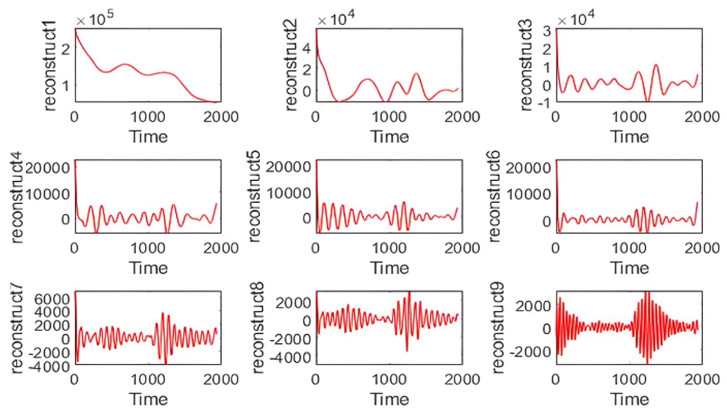
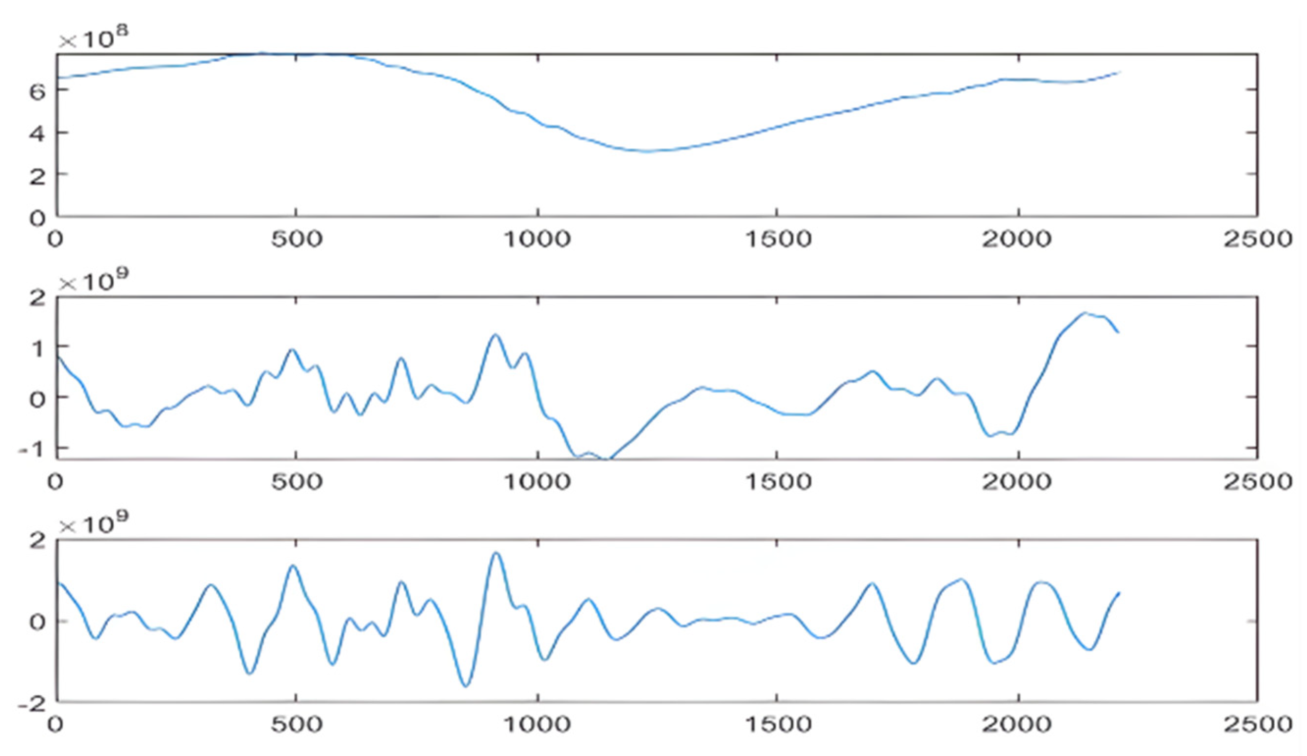
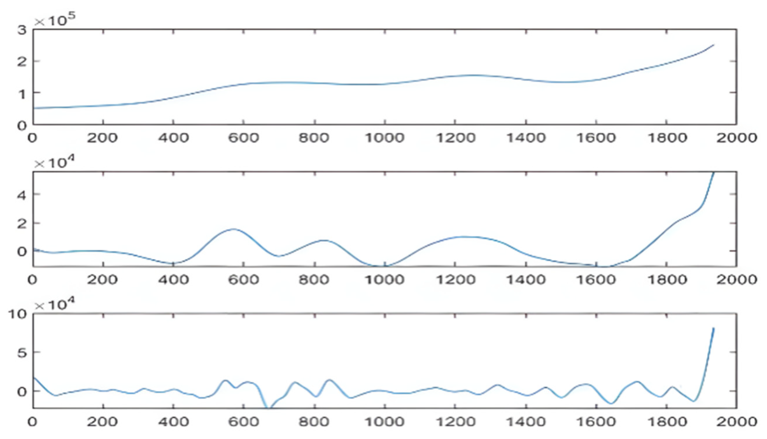
2.1.1. SSA Decomposition

SSA, as an analytical method for studying nonlinear time series, generally includes four parts: embedding, decomposition, grouping and reconstruction. SSA can extract the periodic signal, long-term trends and other information from time series by creating a tracking matrix and decomposing and reconstructing it, and remove noise [35], so it can extract important information of data effectively. In addition, SSA has become an increasingly popular time series filtering and prediction technology. This method has also been proved to be able to solve some defects of machine learning methods. SSA can effectively solve the problem of randomness and difficulty in parameter selection compared with the basic AR model; the SSA-treated model can improve the prediction accuracy of the model [36,37]. The process of applying the SSA analysis method to preprocess energy price series is as follows:

1. For a one-dimensional time series $X=(x_1,\cdots ,x_T)$ of length $T$, set the window length $L(1<L<T/2)$ and construct the trajectory matrix according to Equation (1):

$$X=(x_{ij}{)}_{I,J=1}^{L,M}=\left[\begin{array}{cccc}{x}_1& x_2& \cdots & x_M\\ x_2& x_3& \cdots & x_{M+1}\\ \cdots & \cdots & \cdots & \cdots \\ x_L& x_{L+1}& \cdots & x_T\end{array}\right]$$

(1)

where: $M=T-L+1$.

2. Perform the singular value decomposition of the trajectory matrix $X$. We obtain $L$ eigenvalues ${\lambda }_1,{\lambda }_2,\cdots ,{\lambda }_L$ and the corresponding eigenvectors $U_1,U_2,\cdots ,U_L$ and $d$ is the rank of the trajectory matrix $X$. The decomposition equation is shown in (2) below:

$$X={\displaystyle \sum _{i=1}^d\sqrt{{\lambda }_i}}(U_i{W}_i^T)+{\displaystyle \sum _{i=d+1}^d\sqrt{{\lambda }_i}}(U_i{W}_i^T)\approx {\displaystyle \sum _{i=1}^d\sqrt{{\lambda }_i}}(U_i{W}_i^T)$$

(2)

where: $M=W_i=X^T{U}_i/\sqrt{{\lambda }_i},i=1,2,3,\cdots ,d$.

3. Packet processing: according to the smoothing threshold, choose the first M decomposition in formula 3 with a higher contribution rate than the smoothing threshold.

4. Perform diagonal averaging to transfer the decomposition matrix $X$ into a time series $x_1,x_2,\cdots ,x_k,\cdots ,x_T$.

$${\tilde{x}}^{(i)}=\{\begin{array}{cc}\frac{1}{k}{\displaystyle \sum _{b=1}^k{x}_{b,k-b+1}^{(i)}}& 1\le k\le L^{*}\\ \frac{1}{L^{*}}{\displaystyle \sum _{b=1}^{L^{*}}{x}_{b,k-b+1}^{(i)}}& L^{*}\le k\le K^{*}\\ \frac{1}{T-k+1}{\displaystyle \sum _{b=k-K^{*}+1}^{T-K^{*}+1}{x}_{b,k-b+1}^{(i)}}& K^{*}\le k\le T\end{array}$$

(3)

where: $L^{\ast }=\min (L,K),K^{\ast }=\max (L,K)$.

5. Sum the time series up, and then obtain the smoothed energy resource price series.

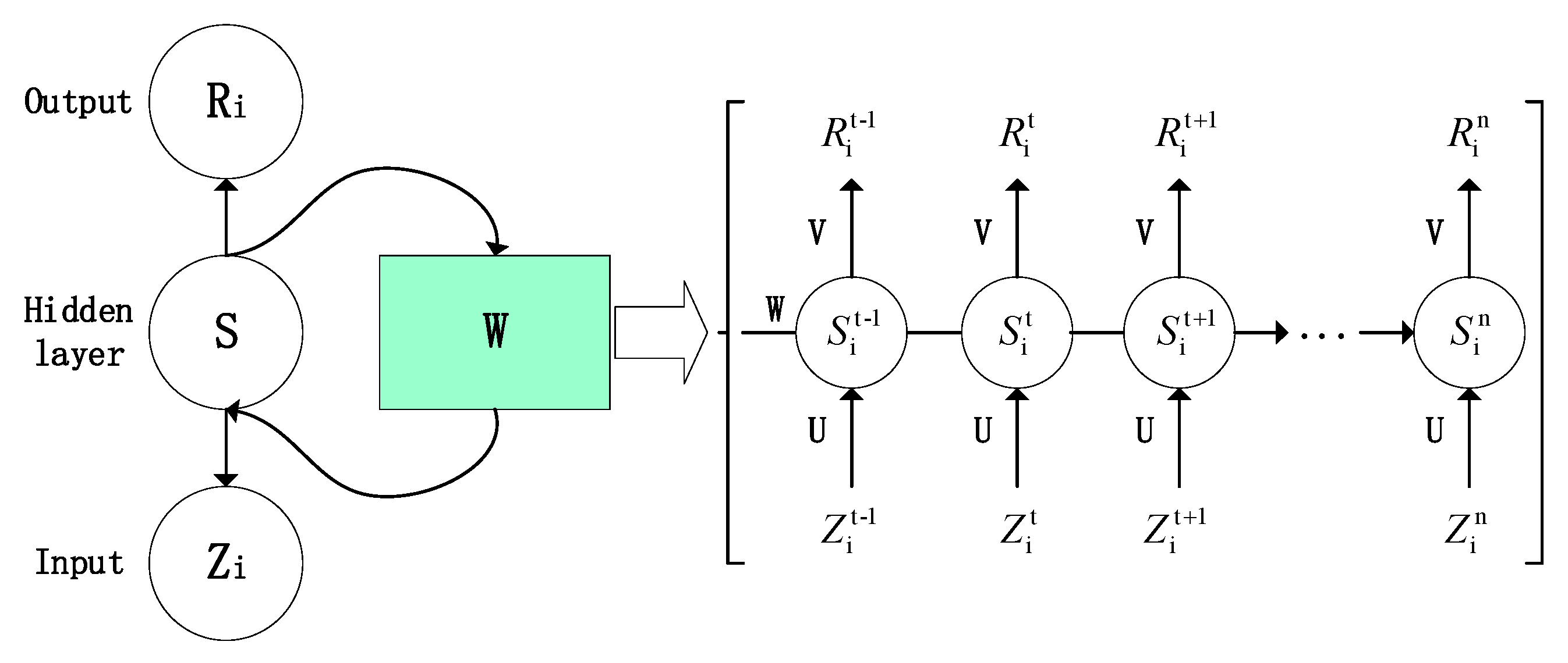
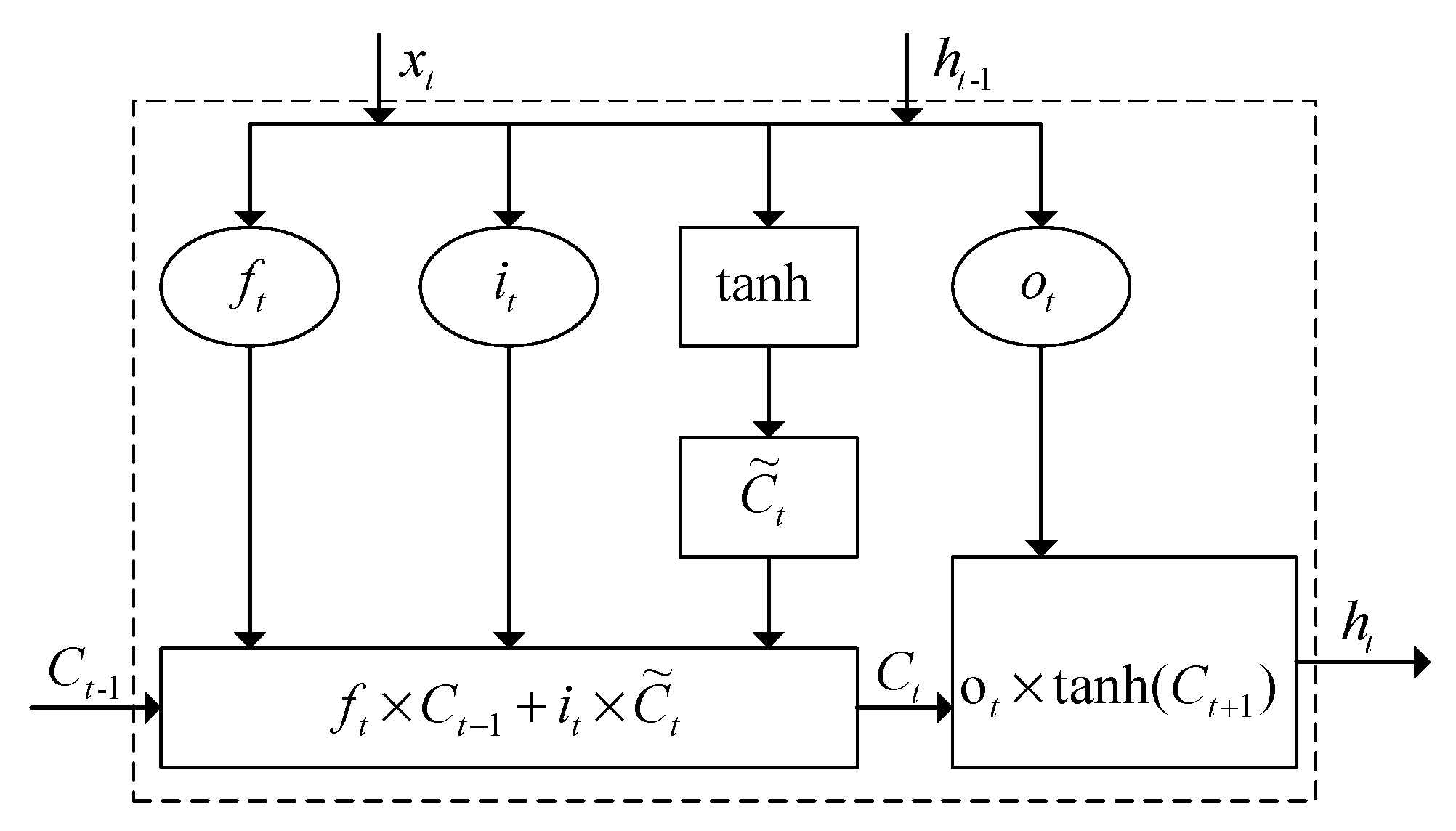
2.1.2. LSTM Neural Network

A RNN is the most common machine learning model in time series prediction. RNNs allow the persistence of information, and are often used to solve the problem of nonlinear time variability, as shown in Figure 1.

For an RNN, the composition could be concluded to be the input layer, hidden layer and output layer. The structure is shown in Figure 1. In Figure 1, the structure is similar to the neural network without W. Hence, the RNN could learn the synergistic effect. For model W, the value $S_t$ of the hidden layer depends not only on the current input $Z_t$ but also on the value $S_{t-1}$ of the last hidden layer. Certainly, model W could learn the interaction among rounds of assessment.

However, the RNN model cannot deal with the long-term data dependence because the gradient disappears in the training process of the model. Input gate, output gate and forget gate are added to the neuron part of the RNN in the LSTM model. Related research by scholars also proves the reliability of the neural network based on LSTM for time series prediction [38,39]. The model is structured as shown in Figure 2.

In Figure 2, $x_t$ is the input vector at time t; $h_t$ represents the output of the current hidden layer; $h_{t-1}$ represents the output of the previous hidden layer; $C_t$ represents the memory cell in the current hidden layer; ${\tilde{C}}_t$ is the state of the memory cell, where the function of memory cell is to control the information transmission in the memory unit; $f_t$ is the forget gate, and is used to control the discarded information; $i_t$ is the input gate that controls the information that needs to be retained; $o_t$ is the output gate, which controls the information that needs to be output.

The equations for $f_t$, $i_t$, $o_t$, ${\tilde{C}}_t$, $C_t$, $h_t$ are as follows:

$$f_t=\sigma (W_f\times [h_{t-1},x_t]+b_f)$$

(4)

$$i_t=\sigma (W_i\times [h_{t-1},x_t]+b_i)$$

(5)

$$o_t=\sigma (W_o\times [h_{t-1},x_t]+b_o)$$

(6)

$${\tilde{C}}_t=\tan (W_c\times [h_{t-1},x_t]+b_c)$$

(7)

$$C_t=f_t\times C_{t-1}+i_t\times {\tilde{C}}_t$$

(8)

$$h_t=o_t\times \tan (C_{t+1})$$

(9)

In Equations (4)–(9), $W_f$, $W_i$, $W_o$ and $W_c$ are the weight matrix, $\sigma$ is the sigmoid function, $b_f$, $b_c$, $b_i$ and $b_o$ are the offset matrix, $\mathrm{sigmoid}$ and $\tan h$ are activation functions.

$$\mathrm{sigmoid}(x)=\frac{1}{1+e^{-x}}$$

(10)

$$\tan h(x)=\frac{e^x-e^{-x}}{e^x+e^{-x}}$$

(11)

2.1.3. Calculation of Carbon Intensity

Carbon intensity is the amount of carbon dioxide (CO₂) emissions per unit of GDP. Zhu et al. [39] and Peng et al. [40] showed the decomposition results of multifactors of carbon emissions: in China, the contribution of economic output effect to carbon emissions is obviously greater than other macrofactors, including energy structure, industrial structure, population size and so on. Therefore, the existing articles mostly use GDP and industrial added value to measure the carbon emission intensity of the whole society [41]. Based on the methods used by Chinese scholars to calculate China’s carbon emission intensity and emissions [42,43], this paper uses China’s macroeconomic indicators and energy consumption from 2011 to 2020 to calculate China’s total social carbon emission intensity. The specific calculation equations are as follows:

$$Q_{c{o}_2}={\displaystyle \sum _{i=1}^n{E}_i}\times S{C}_i\times C{F}_i$$

(12)

$$C{F}_i=C{C}_i\times CO{F}_i\times (44/12)$$

(13)

where $Q_{c{o}_2}$ is the total amount of CO₂ emissions, $E_i$ is the energy consumption of the energy source, $S{C}_i$ is the conversion coefficient of standard coal, $C{F}_i$ is the energy carbon emission coefficient, $C{C}_i$ is the energy carbon content, $CO{F}_i$ is the carbon oxidation factor, and the molecular ratio of carbon dioxide to carbon is 44/22. The conversion coefficient of standard coal is based on the low calorific value from the statistical yearbook of energy, and the carbon emission coefficient refers to the IPCC (2006) standard.

According to the constant GDP of 2003, we calculate the value of “carbon emission intensity”, $F$.

$$F=Q_{C{O}_2}/GDP$$

(14)

Through the above equation, we can obtain the result for China’s carbon dioxide emission intensity.

2.1.4. LVQ Cluster Technology

LVQ is a hybrid network composed of an input layer, competition layer and linear output layer. It is similar to the vector quantization (VQ) method in form, but it is different from the vector quantization method. The traditional vector quantization clustering method is not suitable for nonlinear data, but LVQ clustering is a dynamic clustering method that can effectively solve the above problems. LVQ can correct these reference templates through supervised adaptive learning, and the results will change with the number of iterations.

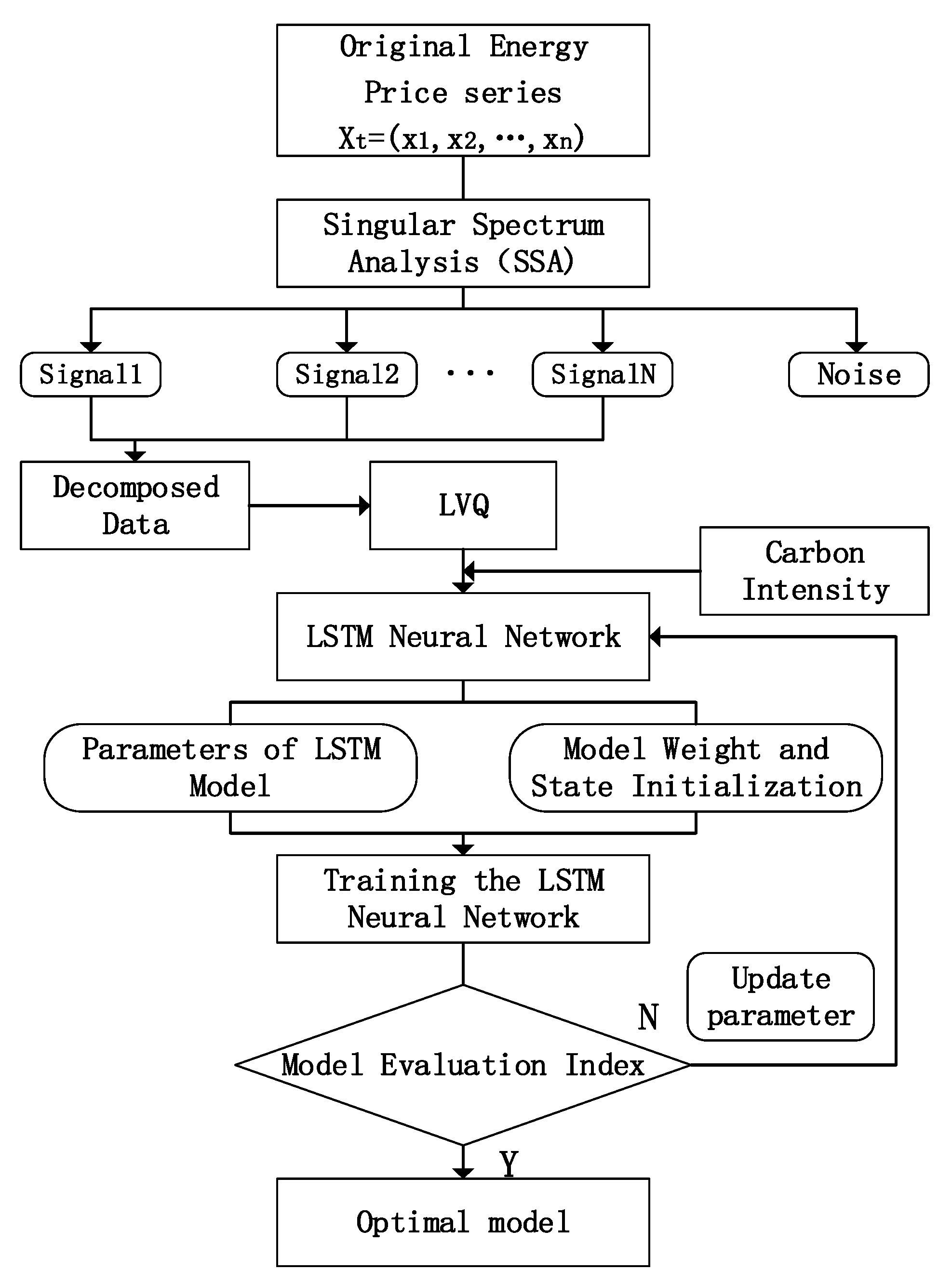
2.2. Construction of SSA-LSTM Model

Some scholars have verified the feasibility of combining the SSA and LSTM methods [44,45]. However, in the field of energy prices, the combination of the decomposition method and machine learning model is rare. The change in energy price is a multifactor process. Whether the combination of SSA and LSTM can effectively predict the energy price or not, and whether this improves the accuracy of the forecast, are also explored in this paper. Therefore, this article chooses to use the SSA-LSTM combined approach to predict energy prices. The SSA-LSTM model is a combination of SSA and the LSTM depth learning network model that breaks down the original energy price series into individual components by SSA. Moreover, an LVQ prototype clustering technique is used to aggregate the decomposed data into price series with different features. Then, we calculate the “carbon emission intensity” factor as the global constraint on the price data. Finally, the “carbon emission intensity” and the reconstructed price data are input into the LSTM neural network model. Through debugging, the optimal model is obtained, and the evaluation index is used to verify the superiority and applicability of the new model. The framework is shown in Figure 3.

The prediction of energy prices with the SSA-LSTM combined model mainly includes three parts:

Step 1: Singular-value decomposition of SLA series.

SSA decomposition is performed on the energy price series and the previous P decomposition is filtered out.

Construct the trajectory matrix: select the window length L and convert the observed one-dimensional data $x_1,\cdots ,x_T$ into the trajectory matrix X.

The matrix X is decomposed by SVD.

Based on the given threshold, the preceding P components are used as substitutes for the original price series, $x_1,\cdots ,x_P$.

Step 2: Refactoring decomposition.

LVQ clustering is used to cluster the decomposition amount into m classes.

According to the results of clustering reconstruction (the same class of components plus), we can obtain the reconstructed sequence.

Step 3: Refactoring decomposition.

The LSTM algorithm is trained by using the lag term of the reconstruction quantity (${\overline{x}}_{i,t-1},\cdots ,{\overline{x}}_{i,t-d}$) as the input and $x_{i,t}$ as the expected output. Finally, we obtain the prediction sequence ${\stackrel{⌢}{x}}_{i,t}$ of clustering reconstruction. In this model, the time window size, batch size, training times and the number of hidden layer units are set as hyperparameters.

2.3. Model Optimization and Comparison

The purpose of this step is to carry out the model optimization and comparison. Hyperparameters in the baseline model usually have a great impact on the prediction accuracy. LSTM has several hyperparameters, e.g., learning rate, the number of iterations, the number of neurons, etc., which affect the robustness and effectiveness of the LSTM model. Inefficient optimization will lead to imperfect models and a poor prediction ability. To overcome this problem, SSA, which has been successfully employed for parameter optimization problems, is used to optimize the parameters of the LSTM model in this work. In order to verify the accuracy of the proposed model, the feasibility of the “decomposition-reconstruction-integration” strategy is firstly verified. Secondly, this model is compared with the current mainstream forecasting models.

3. Empirical Analysis

3.1. Selection of Data Samples and Related Parameters

Considering that the Chinese government first announced its CO₂ emission reduction targets in 2009, the sample data selected in this paper are China’s coke price (trading day) and the average price of PV-grade polysilicon in China (trading day) from September 2011 to September 2020. Coal and polysilicon price data come from China forward database, and energy consumption and GDP data come from China Statistical Yearbook and China Energy Statistical Yearbook. The variables and their summary statistics are shown in

Table 1. Variable and summary statistics.

Variable	Unit	Mean	Std. Dev.	Min	Max
Coal price	CNY 10,000	12.933	5.259	4.590	40.010
Polysilicon price	CNY 10,000	0.159	0.048	0.061	0.267

.

Firstly, we use the time series interpolation algorithm framework (E (2) GAN) to deal with the missing value in the price [46]. E (2) GAN is essentially a denoising autoencoder. The input is a time series containing missing values, generating a complete phase time series. The loss of discriminator is divided into two parts: square error loss and discriminant loss, which are used to make the time series generated by the generator (1) as similar as possible to the original time series (2) and as real as possible. This method is used to deal with missing values. Because the data are all daily data, and the length of the SSA window cannot exceed 1/2 of the sequence number, the length of the decomposition window is 240, and the decomposition threshold is 0.1%. Based on TensorFlow and the Keras deep learning framework, the model for this experiment is constructed.

The time steps of the input layer of the LSTM network are equal to the length of the variable time series of the energy price prediction. Since all the data in this paper are from the price data of the energy trading day, the time steps are initially set as 5 and the dimension of the output layer is set as 1. That is to say, coal and polysilicon price data from days t minus 5 to t minus 1 are predicted from day t, and the dimension of the input layer is the number of variables. The number of hidden layers is the number of LSTM layers. Under certain conditions, the nonlinear fitting ability of the model is directly proportional to the number of hidden layers. The dimension of the hidden layer is generally determined by the following Equation (15).

$$n_3=\sqrt{n_1+n_2}+a$$

(15)

In the equation, $n_1$ and $n_2$ represent the dimension of the input layer and output layer, respectively, and $a$ is the interval constant. According to the empirical formula and several tests, the hidden layer dimension is selected as 7. In order to reduce the influence of human factors on the model, the values of main network parameters are obtained through a series of experiments, as listed in

Table 2. The training parameters of LSTM.

Parameters of the Category	Numerical
Epochs	2000
Learning rate	0.07
Error performance target value	10−6
Hidden layers	7
Hidden units	128

.

3.2. Empirical Results

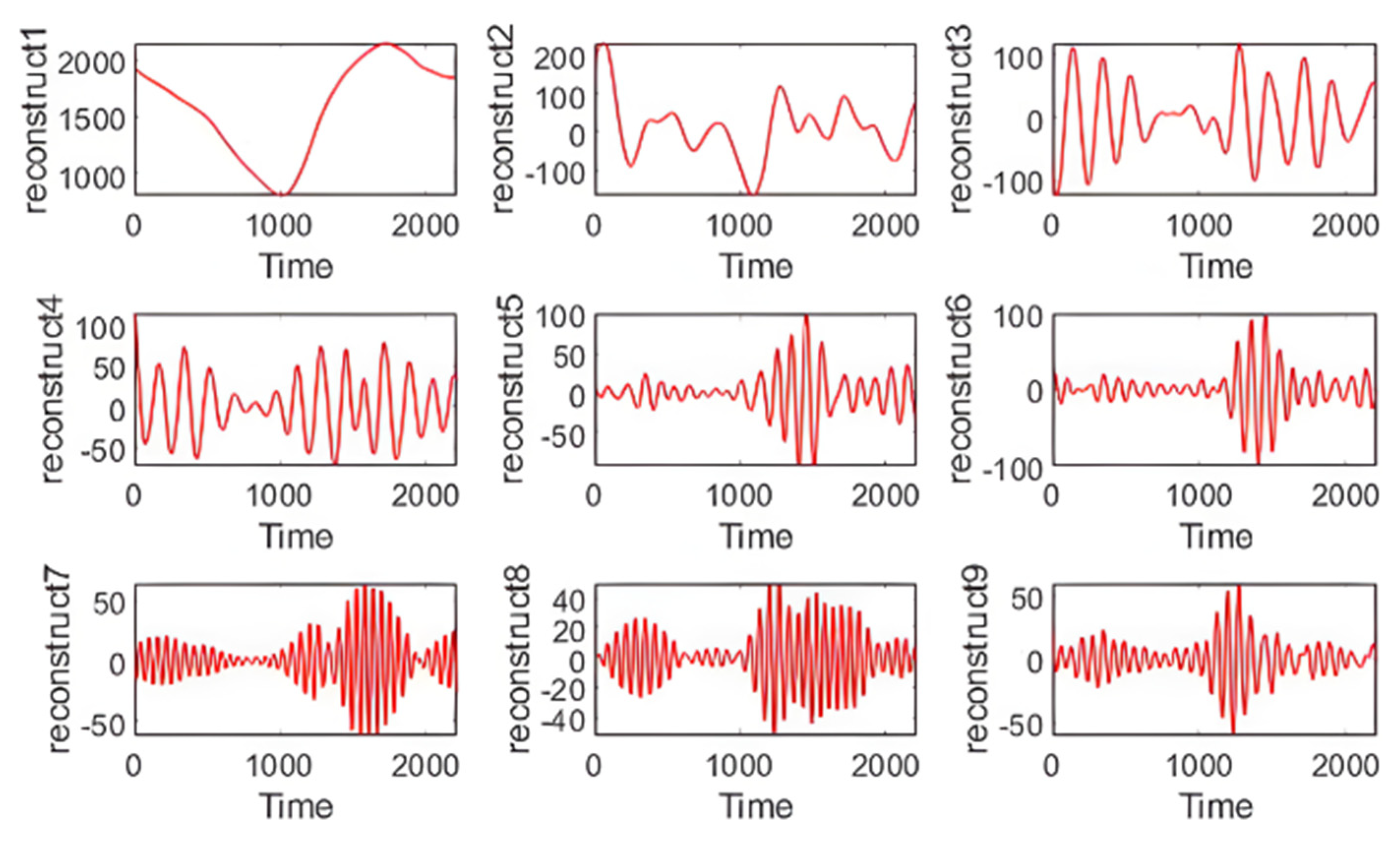
3.2.1. SSA Decomposition and LVQ Cluster

By using SSA to decompose the time series, the reconstructed sequence after SSA decomposition can be obtained. This includes the extraction of trend and periodic information of the original time series by SSA. The specific steps of SSA decomposition are as follows: according to the above, the window length L of SSA decomposition is 240; next, SVD decomposition is performed to generate 240 eigenvalues. The third step is to determine the grouping quantity, M = 30, and its value is the number n when the accumulative sum of the first N eigenvalues reaches 90% of the sum of the eigenvalues. Under the decomposition threshold of 0.1%, nine decomposition quantities are obtained for coal and polysilicon prices, respectively (Figure 4 and Figure 5). In order to obtain the characteristic specific information of energy and resource prices, the above decomposition quantities are clustered using the LVQ method. Finally, signal sequences representing different price characteristics can be obtained. LVQ is a dynamic cluster method, and its clustering results will change with the number of iterations. Therefore, this paper carries out iterative clustering for decomposition quantities of coal and polysilicon for a significant amount of time, and takes the grouping method with the highest frequency as the final clustering result (Figure 6 and Figure 7).

Figure 4 and Figure 5 are the decomposition result of coal and polysilicon prices. The first sequence represents the overall trend of the price of coal and polysilicon, and the last characteristic sequences represent the main fluctuation and periodic information of the price. Figure 6 and Figure 7 are the cluster results of coal and polysilicon prices. In this paper, both coal and polysilicon prices are divided into three categories, which are the first component and the other two components. In Figure 6 and Figure 7, the first sequence represents the overall trend of the price, the second sequence represents the price fluctuation, and the third sequence represents the price cycle. Looking at the price breakdown for both commodities, the volatility components for coal and polysilicon tend to converge around 2015 and around 2020, suggesting that energy prices may be affected by the Paris Agreement target for carbon neutrality.

To perform diagonal averaging, we can obtain the reconstruction time series (Figure 8 and Figure 9). In Figure 8 and Figure 9, the red line is the original price sequence, and the blue line is the reconstructed price sequence. It can be found that the reconstruction quantity obtained under the threshold of 0.1% can explain the main information regarding polysilicon and coal price. Coal prices have continued to rise due to the impact of the world energy crisis since 2020 and China’s “Dual control of energy and consumption” policy. The price of polysilicon decreased continuously until 2015 due to the production capacity. After 2015, the price of polysilicon fluctuated, but it has been in a relatively gentle downward trend.

3.2.2. Calculation of Carbon Intensity

According to the standards and data of the IPCC National Greenhouse Gas Emission Inventory (2006) and China Energy Statistical Yearbook, we calculated the total carbon dioxide emissions produced in the sample period. The above results include eight energy categories: coal, coke, crude oil, gasoline, kerosene, diesel oil, fuel oil and natural gas. The conversion coefficient of standard coal is based on the low calorific value from the Energy Statistical Yearbook, and the carbon emission coefficient is based on the IPCC (2006) standard.

Carbon intensity is calculated on the basis of a constant price GDP for 2011. The value of carbon intensity, F, is shown in

Table 3. China’s carbon intensity table for 2011–2020.

Serial Number	Year	GDP (CNY trillion)	Total Amount of CO2 Emission (Ten Million Tons)	Carbon Intensity	Primary Sector of the Economy	Secondary Sector of the Economy	Tertiary Sector of the Economy
1	2011	47.156	945.940	0.021	0.970	87.150	11.880
2	2012	51.932	1002.690	0.019	0.950	86.980	12.070
3	2013	58.802	1019.770	0.016	1.010	86.410	12.580
4	2014	63.646	1004.830	0.015	1.060	85.900	13.030
5	2015	67.671	975.760	0.013	1.110	84.670	14.220
6	2016	74.413	961.160	0.012	1.160	84.180	14.660
7	2017	82.712	971.450	0.010	1.180	84.000	14.830
8	2018	91.928	1002.750	0.009	1.200	83.750	15.050
9	2019	99.087	1025.670	0.008	1.180	84.070	14.760
10	2020	101.599	1052.020	0.009	1.220	84.510	14.280

. The results show that the development of the energy industry in China’s 12th and 13th “Five-year plans” has achieved a remarkable effect. During 2011–2020, the carbon emission level of all of China was reduced continuously. This paper attempts to add carbon intensity to the prediction model as the overall constraint of the reconstruction price. This is because the national energy and emission reduction policies are not easy to measure as factors affecting prices. However, the policy effects can be reflected in energy supply and demand and economic output. Therefore, this paper takes the carbon emission intensity index as the overall constraint of the reconstructed price, and inputs it together with the price sequence into the LSTM. The neural network can learn the price information and coefficient data corresponding to the characteristics to predict future energy prices.

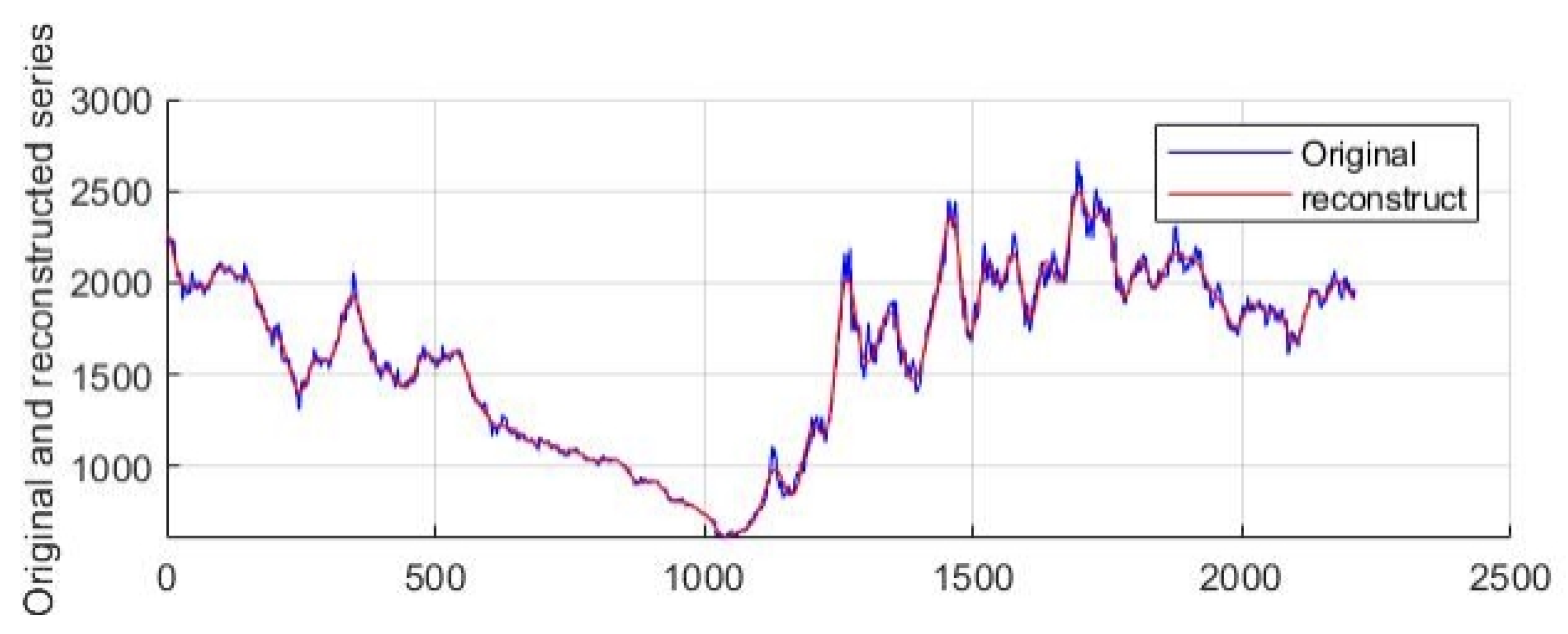
3.2.3. Analysis of Forecast Results

In order to better evaluate the prediction effect of the model, this paper divides the dataset into a training set (the first 80%) and a test set (the last 20%), and uses a variety of evaluation indicators. We select RMSE, MAE, MAPE and R-squared to evaluate the prediction effect of absolute price (the smaller the value, the higher the accuracy). According to the previous analysis, the number of hidden layers of the LSTM is set to 7, the number of neurons in each layer is set to 128, and the number of neurons in the output layer is set to 1. In order to better determine the number of times the LSTM layer is accessed, this paper designs corresponding comparative tests. The influence of different lag days on the prediction effect of the model is judged through experiments, and the optimal value is selected. When training the network, the epoch value is set to 2000. In addition, when the performance of the model on the validation set is not improved for 140 consecutive epochs, the training is terminated in advance. The lag days are selected from the set {1, 3, 5, 7, 10, 14}. The prediction results of the model for the test set are shown in

Table 4. Effect of different lag days on model prediction.

Energy Category	Lag Days	1	3	5	7	10	14
Coal	RMSE	0.102	0.097	0.095	0.096	0.113	0.102
	MAE	0.052	0.054	0.051	0.048	0.068	0.063
	MAPE	0.059	0.062	0.058	0.058	0.063	0.077
	R-squared	0.714	0.685	0.755	0.734	0.721	0.611
Polysilicon	RMSE	0.092	0.086	0.087	0.094	0.102	0.099
	MAE	0.073	0.058	0.059	0.064	0.074	0.101
	MAPE	0.051	0.043	0.042	0.039	0.071	0.094
	R-squared	0.812	0.825	0.852	0.771	0.688	0.652

below.

It can be seen from Table 4 that when there are five lag days, the model has the best prediction effect on the test set. It can be found that if the lag days are too short, the model will fall into the local optimal solution. If the lag days are too long, the increase in model complexity does not bring about the same improvement in prediction accuracy.

After setting up the model, in order to verify the feasibility of the “decomposition-reconstruction-integration” strategy proposed in this paper in detail, the following comparative experiments are proposed. We input the original price data, the decomposed price data of SSA, the decomposed and clustered price data and the clustered data with the constraint of carbon intensity into the LSTM model separately.

Table 5. Analysis of model prediction results.

Energy Category	Input Value	RMSE	MAE	MAPE	R-Squared
Coal	P1	0.135	0.087	0.072	0.643
	P2	0.118	0.064	0.067	0.654
	P3	0.098	0.054	0.065	0.725
	P4	0.095	0.051	0.058	0.755
Polysilicon	P1	0.121	0.068	0.069	0.732
	P2	0.086	0.061	0.053	0.812
	P3	0.086	0.064	0.048	0.824
	P4	0.087	0.059	0.042	0.831

P1 is the original price data; P2 is the decomposed price data of SSA; P3 is using LVQ cluster method to cluster SSA decomposition quantity; P4 is the addition of carbon intensity on the basis of P3 as a constraint condition.

shows the forecast results of coal and polysilicon prices. RMSE, MAE, MAPE and R-square indicators all show that the comprehensive prediction effect of data after SSA decomposition and LVQ clustering is better. After adding the constraint of “carbon emission intensity”, the prediction accuracy is further improved. (1) The evaluation index value of P2 is less than that of P1, indicating that the prediction effect based on the SSA decomposition model is better than that using only original data. There may be a nonlinear relationship between energy price information and its own lag term. The original price data cannot effectively predict the trend of energy price. (2) The evaluation index values of P3 are mostly smaller than those of P2, indicating that the SSA-LSTM model combined with LVQ clustering has a better prediction effect on most indicators. The decomposition–cluster strategy has a better prediction effect and can reflect energy price level and real fluctuation more effectively. (3) By analyzing the two cases with and without a carbon intensity constraint, we find that the prediction effect is better under the carbon emission constraint. It shows that in the macroforecast of energy price, against the background of carbon neutrality, considering “carbon emission intensity” as the overall constraint of leading market can effectively explore the regular characteristics of energy price information.

According to the above analysis, it can be seen that the prediction results based on the “decomposition-reconstruction-integration” strategy are better than those based solely on historical data. After adding carbon intensity, we can see that the prediction effect of the model is better. This is because the decomposition clustering of energy prices can provide an intuitive window in which to analyze the characteristics of prices and external shocks, and improve the accuracy of the model. The addition of the carbon intensity coefficient can help us analyze and judge the historical situation in the context of carbon neutrality and deal with the large price fluctuations caused by the international environment, energy supply and demand, energy policy and other factors.

Figure 10 and Figure 11 show the white noise of coal and polysilicon prices. Figure 12 and Figure 13 show the comparison of the predicted and actual values of coal and polysilicon prices (the first is the LSTM prediction, followed by the SSA-LSTM prediction). In the figure, the horizontal axis represents days and the vertical axis represents prices. The blue line represents the true value of the model, and the red line represents the predicted value of the model. By comparing Figure 12 and Figure 13, it can be found that when the original price is not processed, the actual value of the prediction model differs greatly from the predicted value. This phenomenon is particularly obvious in the middle- and late-stage data. Since the signing of the Paris Agreement in 2015, the LSTM model has obviously been less accurate than the SSA-LSTM model. This shows that prediction based only on historical data will lead to a poor prediction effect for the model. This may be because the price of energy, a very important natural resource, is susceptible to the influence of macropolicies, market sentiment and emergencies. Therefore, the prediction of price based on features only from historical data will inevitably lag behind the prediction of emergencies, resulting in the predicted value lagging behind the real fluctuation value. This paper processes energy price data based on the “decomposition-integration-reconstruction” strategy, and takes the carbon emission index as a constraint condition, which greatly improves the prediction performance of the hybrid model.

Overall, the model has a high accuracy in predicting energy prices. This model can effectively capture the energy price fluctuations from 2011 to 2020. Before 2015, the coal price had been declining. After 2015, the coal price continued to maintain an upward trend despite slight fluctuations. As for polysilicon prices, it was in a slow downward trend during the transformation of the global energy industry. In addition, the model captured the inflection point of two types of prices, accurately predicting the peak of coal prices at that stage.

4. Comparative Analysis with Other Mainstream Time Series Prediction Models

Traditional time series analysis (AR), machine learning method support vector machine (SVR), the decision tree method (DT) and the artificial intelligence method BP neural network (NN) are widely used in different fields of time series prediction. We compared the performance indices of the SSA-LSTM combined neural network prediction model with those of the above four mainstream time series prediction models and used RMSE, MAE and R-squared value for evaluation. The final detailed results are shown in Table 5. It can be seen that the SSA-LSTM model has the best effect.

For the “decomposition-reconstruction-integration” model of coal, the RMSE value is 0.095, the MAE value is 0.051, and the R-squared value is 0.755. In terms of the RMSE index, the SSA-LSTM model is better, but how it differs from the other three models is not obvious. The RMSE values are all in the range of [0.090, 0.309]. In terms of the MAE index, there is no obvious difference between the SSA-LSTM model and the other four models. The MAE values are all within the range [0.050, 0.270], but the SSA-LSTM model has the smallest error. In terms of the R-squared index, the SSA-LSTM model can reach 0.755, while the BPNN algorithm is only 0.559. The R-squared values of the other two algorithms are within the range [0.550, 0.610]. Similarly, for the polysilicon price prediction model, the SSA-LSTM model had a better prediction effect.

In addition, in this section, we compare the model based on the “decomposition-reconstruction-integration” strategy with the model based on the “decomposition-integration” strategy, as shown in

Table 6. Results of model prediction and evaluation index.

Energy Category	Index	“Decomposition-Integration” Model				“Decomposition-Reconstruction-Integration” Model
		SSA- LSTM	SSA- BPNN	SSA- RNN	SSA- SVR	SSA- LSTM	SSA- BPNN	SSA- RNN	SSA- SVR
Coal	RMSE	0.118	0.284	0.269	0.331	0.095	0.205	0.2213	0.309
	MAE	0.064	0.198	0.184	0.275	0.051	0.152	0.162	0.268
	R-squared	0.654	0.658	0.598	0.501	0.755	0.559	0.601	0.590
Polysilicon	RMSE	0.086	0.191	0.221	0.224	0.087	0.197	0.213	0.212
	MAE	0.061	0.166	0.171	0.298	0.059	0.160	0.171	0.268
	R-squared	0.812	0.832	0.604	0.543	0.831	0.735	0.684	0.595

below. From the evaluation value, we can find that the “decomposition-reconstruction-integration” model is more accurate than the “decomposition-integration” model.

To sum up, we can find that the strategy based on “decomposition-reconfiguration-integration” is superior to the traditional “decomposition-integration”. The same is true for other machine learning models. Therefore, the model can reflect the complex relationship between the price of coal and polysilicon and the influencing factors well. However, we also found that the accuracy was higher in predicting the price of energy coal, but some indicators showed lower accuracy in predicting the price of polysilicon.

5. Discussion

In the international energy market, fluctuations in energy prices will affect the economic development trend of a country. Therefore, it is very important to predict energy prices more accurately. At present, price time series are usually divided into deterministic trends, deterministic cycles, residual components and white noise [47]. Then, the original time series can be fitted and extrapolated to predict the future price and other changes in the trend. Against the background of carbon neutrality, this paper proposes a new energy price forecasting model based on the strategy of “decomposition-reconstruction-integration”. This strategy optimizes the model from the background value direction. This model can effectively solve the time-delay problem and dynamic problem of energy price. The decomposition method it uses also makes up for the lack of a direct application of a deep learning model to predict energy prices in the past.

Against the background of carbon neutrality, this paper constructs the SSA-LSTM model based on the strategy of “decomposition-reconstruction-integration” to predict the change trend of energy prices with carbon emission intensity as the constraint. The results show that the prediction accuracy of this model is higher. For coal price, the RMSE value decreased from 0.135 to 0.098, the MAE value decreased from 0.087 to 0.054, the MAPE value decreased from 0.072 to 0.064, and the R-squared value increased from 0.643 to 0.725. Regarding polysilicon prices, the RMSE value decreased from 0.121 to 0.096, the MAE value decreased from 0.068 to 0.064, the MAPE value decreased from 0.069 to 0.048, and the R-squared value increased from 0.718 to 0.764.

The article also has the corresponding limitation regarding the energy price decomposition method and the reconstruction method, which only used the SSA and LVQ. It did not explore whether other methods could further improve the accuracy of price forecasts. Whether this strategy can also be applied to other areas has not been explored. In addition, due to the availability of data, the analysis of energy prices only focuses on China’s energy price data. Whether the survey results also apply to international energy prices needs to be analyzed separately. There are many factors that affect fluctuation in energy prices, such as policy changes, the interaction between energy structure and new energy. Therefore, in future work we hope to reasonably establish relevant prediction models suitable for energy prices by analyzing different influencing factors.

6. Conclusions

Against the background of carbon neutrality, this paper constructs the SSA-LSTM mixed prediction model by considering carbon emission intensity as the constraint condition. The hybrid model can effectively predict the changing trend of different energy prices. The main conclusions are as follows:

This paper’s multiscale combination prediction model relies on the “decomposition-reconstruction-integration” strategy. The data were decomposed by SSA and dynamically clustered utilizing the LVQ prototype clustering technology. The model’s input variables are the original decomposition sequence representing the price sequence’s overall trend and the fluctuations in different cycles. Then, we input the decomposed and reconstructed data into the LSTM model for training. The SSA-LSTM hybrid model can effectively predict the changing trend of different energy prices. Compared with the energy price prediction model that was not a hybrid model, the error of the proposed SSA-LSTM hybrid prediction model based on the carbon constraint is reduced from 2% [48,49] to about 1%, while the prediction accuracy is higher.

Considering the carbon intensity coefficient as an external influencing factor enhances the prediction accuracy for energy price fluctuations under carbon neutrality. Since the information provided by energy price data is relatively limited, it is difficult to comprehensively provide the current economic and social situation. Therefore, to consider the impact of carbon emissions on the price of natural resources within the context of carbon neutrality, we used GDP, energy supply and industrial added value to calculate the carbon intensity coefficient. As the overall constraints of leading markets are added to the model, the results reveal that the model becomes more accurate, complementing the research results of Ma et al. [50] and Zeng et al. [51]. Moreover, we found a specific correlation between carbon emissions and energy prices. Thus, carbon emissions should be considered in future research on energy prices.

Traditional energy price prediction methods mostly predict fossil energy prices. Although some scholars have predicted the price of new energy types, they employed traditional prediction models, which present significant prediction errors. Against the background of “carbon neutrality” and “dual control of energy consumption”, the proposed SSA-LSTM model can effectively predict the price of traditional energy and match the price prediction of solar energy and other new energy types. Hence, our prediction model complements the diverse range of existing energy price forecasting methods.

References

1. Birkenberg, A.; Narjes, M.E.; Weinmann, B.; Birner, R. The potential of carbon neutral labeling to engage coffee consumers in climate change mitigation. J. Clean. Prod. 2021, 278, 123621. [Google Scholar] [CrossRef]
2. Wu, S.; Hu, S.; Frazier, A.E. Spatiotemporal variation and driving factors of carbon emissions in three industrial land spaces in China from 1997 to 2016. Technol. Forecast. Soc. Change 2021, 169, 120837. [Google Scholar] [CrossRef]
3. Cheng, J.; Yi, J.; Dai, S.; Xiong, Y. Can Low-Carbon city construction facilitate green growth? Evidence from China’s pilot Low-Carbon city initiative. J. Clean. Prod. 2019, 231, 1158–1170. [Google Scholar] [CrossRef]
4. Li, Y.; Shen, J.; Xia, C.; Xiang, M.; Cao, Y.; Yang, J. The impact of urban scale on carbon metabolism—A case study of Hangzhou, China. J. Clean. Prod. 2021, 292, 126055. [Google Scholar] [CrossRef]
5. Xu, G.; Schwarz, P.; Yang, H. Determining China’s CO2 emissions peak with a dynamic nonlinear artificial neural network approach and scenario analysis. Energy Policy 2019, 128, 752–762. [Google Scholar] [CrossRef]
6. Zeng, S.; Su, B.; Zhang, M.; Gao, Y.; Liu, J.; Luo, S.; Tao, Q. Analysis and forecast of China’s energy consumption structure. Energy Policy 2021, 159, 112630. [Google Scholar] [CrossRef]
7. Gao, J.; Guan, C.; Zhang, B.; Li, K. Decreasing methane emissions from China’s coal mining with rebounded coal production. Environ. Res. Lett. 2021, 16, 1–10. [Google Scholar] [CrossRef]
8. Yang, F.-f.; Zhao, X.-g. Policies and economic efficiency of China’s distributed photovoltaic and energy storage industry. Energy 2018, 154, 221–230. [Google Scholar] [CrossRef]
9. Si, R.; Aziz, N.; Raza, A. Short and long-run causal effects of agriculture, forestry, and other land use on greenhouse gas emissions: Evidence from China using VECM approach. Environ. Sci. Pollut. Res. 2021, 28, 64419–64430. [Google Scholar] [CrossRef]
10. Coppola, A. Forecasting oil price movements: Exploiting the information in the futures market. J. Futures Mark. 2008, 28, 34–56. [Google Scholar] [CrossRef]
11. Zhang, Y.-J.; Wang, J. Exploring the WTI crude oil price bubble process using the Markov regime switching model. Phys. A-Stat. Mech. Its Appl. 2015, 421, 377–387. [Google Scholar] [CrossRef]
12. Li, Y.; Zhu, Z.; Kong, D.; Han, H.; Zhao, Y. EA-LSTM: Evolutionary attention-based LSTM for time series prediction. Knowl. -Based Syst. 2019, 181, 104785. [Google Scholar] [CrossRef] [Green Version]
13. Garcia-Martos, C.; Caro, E.; Sanchez, M.J. Electricity price forecasting accounting for renewable energies: Optimal combined forecasts. J. Oper. Res. Soc. 2015, 66, 871–884. [Google Scholar] [CrossRef] [Green Version]
14. Wang, J.; Wang, J. Forecasting energy market indices with recurrent neural networks: Case study of crude oil price fluctuations. Energy 2016, 102, 365–374. [Google Scholar] [CrossRef]
15. Chatvorawit, P.; Sattayatham, P.; Premanode, B. Improving Stock Price Prediction with SVM by Simple Transformation: The Sample of Stock Exchange of Thailand (SET). Thai J. Math. 2016, 14, 553–563. [Google Scholar]
16. Chiroma, H.; Abdulkareem, S.; Herawan, T. Evolutionary neural network model for west texas intermediate crude oil price prediction. Appl. Energy 2015, 142, 266–273. [Google Scholar] [CrossRef]
17. Wang, J.; Li, X. A combined neural network model for commodity price forecasting with SSA. Soft Comput. 2018, 22, 5323–5333. [Google Scholar] [CrossRef]
18. Jing, N.; Wu, Z.; Wang, H. A hybrid model integrating deep learning with investor sentiment analysis for stock price prediction. Expert Syst. Appl. 2021, 178, 115019. [Google Scholar] [CrossRef]
19. Rezaei, H.; Faaljou, H.; Mansourfar, G. Stock price prediction using deep learning and frequency decomposition. Expert Syst. Appl. 2021, 169, 114332. [Google Scholar] [CrossRef]
20. Zhang, J.-L.; Zhang, Y.-J.; Zhang, L. A novel hybrid method for crude oil price forecasting. Energy Econ. 2015, 49, 649–659. [Google Scholar] [CrossRef]
21. Reboredo, J.C.; Rivera-Castro, M.A. A wavelet decomposition approach to crude oil price and exchange rate dependence. Econ. Model. 2013, 32, 42–57. [Google Scholar] [CrossRef]
22. Qu, X.M.; Liu, T.T.; Destech Publicat, I. The Impulse Response Analysis of Energy Price on Carbon Intensity Based on VAR Model-Taking Shanxi Province as an Example. In Proceedings of the International Conference on Advanced Management Science and Information Engineering (AMSIE), Hong Kong, China, 20–21 September 2015; ISBN 978-1-60595-246-8. [Google Scholar]
23. Li, W.; Sun, W.; Li, G.; Jin, B.; Wu, W.; Cui, P.; Zhao, G. Transmission mechanism between energy prices and carbon emissions using geographically weighted regression. Energy Policy 2018, 115, 434–442. [Google Scholar] [CrossRef]
24. Jiang, S.; Guo, J.; Yang, C.; Ding, Z.; Tian, L. Analysis of the relative price in China’s energy market for reducing the emissions from consumption. Energies 2017, 10, 656. [Google Scholar] [CrossRef] [Green Version]
25. Sadorsky, P. Forecasting solar stock prices using tree-based machine learning classification: How important are silver prices? North Am. J. Econ. Financ. 2022, 61, 101705. [Google Scholar] [CrossRef]
26. Meng, A.; Wang, P.; Zhai, G.; Zeng, C.; Chen, S.; Yang, X.; Yin, H. Electricity price forecasting with high penetration of renewable energy using attention-based LSTM network trained by crisscross optimization. Energy 2022, 254, 124212. [Google Scholar] [CrossRef]
27. Wu, Y.X.; Wu, Q.B.; Zhu, J.Q. Improved EEMD-based crude oil price forecasting using LSTM networks. Phys. A: Stat. Mech. Its Appl. 2019, 516, 114–124. [Google Scholar] [CrossRef]
28. Siddiqui, A.W. Predicting natural gas spot prices using artificial neu-ral network. In Proceedings of the 2019 2nd International Conference on Computer Applications & Information Security (ICCAIS), Riyadh, Saudi Arabia, 1–3 May 2019; pp. 1–6. [Google Scholar]
29. Windler, T.; Busse, J.; Rieck, J. One month-ahead electricity price forecasting in the context of production planning. J. Cleaner Prod. 2019, 238, 117910. [Google Scholar] [CrossRef]
30. Lu, H.; Ma, X.; Huang, K.; Azimi, M. Carbon trading volume and price forecasting in China using multiple machine learning models. J. Cleaner Prod. 2020, 249, 119386. [Google Scholar] [CrossRef]
31. Zhang, H.; Yang, Y.; Zhang, Y.; He, Z.; Yuan, W.; Yang, Y.; Qiu, W.; Li, L. A combined model based on SSA, neural networks and LSSVM for short-term electric load and price forecasting. Neural Comput. Appl. 2021, 33, 773–788. [Google Scholar] [CrossRef]
32. Yang, Y.; Dong, J.; Sun, X.; Lima, E.; Mu, Q.; Wang, X. A CFCC-LSTM Model for Sea Surface Temperature Prediction. IEEE Geosci. Remote Sens. Lett. 2018, 15, 207–211. [Google Scholar] [CrossRef]
33. Ma, C.; Li, S.; Wang, A.; Yang, J.; Chen, G. Altimeter Observation-Based Eddy Nowcasting Using an Improved Conv-LSTM Network. Remote Sens. 2019, 11, 783. [Google Scholar] [CrossRef]
34. Zhang, Y.; Tao, P.; Wu, X.; Yang, C.; Han, G.; Zhou, H.; Hu, Y. Hourly Electricity Price Prediction for Electricity Market with High Proportion of Wind and Solar Power. Energies 2022, 15, 1345. [Google Scholar] [CrossRef]
35. Afshar, K.; Bigdeli, N. Data analysis and short term load forecasting in Iran electricity market using singular spectral analysis (SSA). Energy 2011, 36, 2620–2627. [Google Scholar] [CrossRef]
36. Sun, M.; Li, X.; Kim, G. Precipitation analysis and forecasting using singular spectrum analysis with artificial neural networks. Clust. Comput. J. Netw. Softw. Tools Appl. 2019, 22, 12633–12640. [Google Scholar] [CrossRef]
37. Liu, H.; Mi, X.; Li, Y.; Duan, Z.; Xu, Y. Smart wind speed deep learning based multi-step forecasting model using singular spectrum analysis, convolutional Gated Recurrent Unit network and Support Vector Regression. Renew. Energy 2019, 143, 842–854. [Google Scholar] [CrossRef]
38. Urolagin, S.; Sharma, N.; Datta, T.K. A combined architecture of multivariate LSTM with Mahalanobis and Z-Score transformations for oil price forecasting. Energy 2021, 231, 120963. [Google Scholar] [CrossRef]
39. Zhu, Q.; Peng, X.; Lu, Z.; Wu, K. Factors decomposition and empirical analysis of variations in energy carbon emission in China. Resources Science 2009, 31, 2072–2079. [Google Scholar]
40. Peng, L.; Li, N.; Zheng, Z.; Li, F.; Wang, Z. Spatial-temporal heterogeneity of carbon emissions and influencing factors on household consumption of China. China Environ. Sci. 2021, 41, 463–472. [Google Scholar]
41. Chen, H.; Qi, S.; Tan, X. Decomposition and prediction of China’s carbon emission intensity towards carbon neutrality: From perspectives of national, regional and sectoral level. Sci. Total Environ. 2022, 825, 153839. [Google Scholar] [CrossRef]
42. Zeng, S.; Zhang, M. Green investment, carbon emission intensity and high-quality economic development: Testing non-linear relationship with spatial econometric model. West Forum 2021, 31, 69–84. [Google Scholar]
43. Wang, Y.; Liao, M.; Wang, Y.; Xu, L.; Malik, A. The impact of foreign direct investment on China’s carbon emissions through energy intensity and emissions trading system. Energy Econo. 2021, 97, 105212. [Google Scholar] [CrossRef]
44. Stratigakos, A.; Bachoumis, A.; Vita, V.; Zafiropoulos, E. Short-Term Net Load Forecasting with Singular Spectrum Analysis and LSTM Neural Networks. Energies 2021, 14, 4107. [Google Scholar] [CrossRef]
45. Han, M.; Zhong, J.; Sang, P.; Liao, H.; Tan, A. A Combined Model Incorporating Improved SSA and LSTM Algorithms for Short-Term Load Forecasting. Electronics 2022, 11, 1835. [Google Scholar] [CrossRef]
46. Luo, Y.; Zhang, Y.; Cai, X.; Yuan, X. E2GAN: End-to-End Generative Adversarial Network for Multivariate Time Series Imputation. In Proceedings of the 28th International Joint Conference on Artificial Intelligence, Macao, China, 10–16 August 2019; pp. 3094–3100. [Google Scholar]
47. Zhao, J.; Cai, R.; Sun, W. Regional sea level changes prediction integrated with singular spectrum analysis and long-short-term memory network. Adv. Space Res. 2021, 68, 4534–4543. [Google Scholar] [CrossRef]
48. Lu, H.F.; Ma, X.; Ma, M.D.; Zhu, S.L. Energy price prediction using data-driven models: A decade review. Comput. Sci. Rev. 2021, 39, 100356. [Google Scholar] [CrossRef]
49. Duan, H.; Liu, Y. Research on a grey prediction model based on energy prices and its applications. Comput. Ind. Eng. 2021, 162, 107729. [Google Scholar] [CrossRef]
50. Ma, Y.; Zhang, L.; Song, S.; Yu, S. Impacts of Energy Price on Agricultural Production, Energy Consumption, and Carbon Emission in China: A Price Endogenous Partial Equilibrium Model Analysis. Sustainability 2022, 14, 3002. [Google Scholar] [CrossRef]
51. Zeng, S.; Zhang, H.; Qu, Y.; Zeng, B. Study on Price Fluctuation and Influencing Factors of Regional Carbon Emission Trading in China under the Background of High-quality Economic Development. Int. Energy J. 2021, 21, 201–211. [Google Scholar]
Figure 1. Expansion diagram of RNN.
Energies 15 08128 g001
Figure 2. LSTM single-neuron structure.
Energies 15 08128 g002
Figure 3. Framework of SSA-LSTM.
Energies 15 08128 g003
Figure 4. Decomposition result of coal price.
Energies 15 08128 g004
Figure 5. Decomposition result of polysilicon price.
Energies 15 08128 g005
Figure 6. Cluster result of coal price.
Energies 15 08128 g006
Figure 7. Cluster result of polysilicon price.
Energies 15 08128 g007
Figure 8. Coal price reconstruction.
Energies 15 08128 g008
Figure 9. Polysilicon price reconstruction.
Energies 15 08128 g009
Figure 10. Coal price white noise.
Energies 15 08128 g010
Figure 11. Polysilicon price white noise.
Energies 15 08128 g011
Figure 12. Prediction effect of coal price.
Energies 15 08128 g012
Figure 13. Prediction effect of polysilicon price.
Energies 15 08128 g013