Heat Conduction with Krylov Subspace Method Using FEniCSx

Abstract

The study of heat transfer deals with the determination of the rate of heat energy transfer from one system to another driven by a temperature gradient. It can be observed in many natural phenomena and is often the fundamental principle behind several engineering systems. Heat transfer analysis is necessary while designing any product. The most common numerical method used to analyze heat transfer is the finite element method. This paper uses the finite element method to demonstrate steady and transient heat conduction in a three-dimensional bracket. The goal here was to determine the temperature distribution and rate of heat flow in the solid. This is crucial in designing machine elements as they are subjected to various thermal loads during operation and also due to fluctuations in the surrounding environmental conditions. The temperature significantly affects stress, displacements, and volumetric strains. Thus, to analyze thermal stresses induced in a machine element, it is necessary to find the temperature field first. The thermal analysis was performed using the open-source package FEniCSx on Python. The program was run using a preconditioned Krylov subspace method for higher-order function spaces. The Krylov subspace solver drastically reduces computational time. The time taken for the execution of each order was recorded and presented.

1. Introduction

Heat conduction can be observed in many natural phenomena and is essential while designing many engineering systems. It is categorized as steady and transient. Processes are simpler to study when they are stable since complicated transient characteristics are avoided and they can still manage to offer accurate answers to our questions. Thus, they are analyzed under some assumed steady conditions, even though most heat transfer issues in practice are transient [1]. Finite element analysis speeds up design and development by lowering the number of physical tests, which also cuts down on the cost and duration of prototyping and testing [2]. The finite element method (FEM) solves and finds solutions to field problems that arise in engineering and mathematical modeling using numerical methods [3]. Problem areas of interest include fluid flow, heat transfer, mass transfer, electromagnetism, etc. Solving such problems requires the spatial distribution of dependent variables to be determined. They can be described either by partial differential equations or integral expressions [4]. Many mechanical problems are governed by partial differential equations (PDEs). FEM solves these PDEs by dividing the geometry into small elements (discretization) and using numerical methods to give an approximate solution with minimum error [5,6]. This paper demonstrates steady and transient heat conduction in a three-dimensional bracket using FEniCSx [7,8]. FEniCSx is an open-source package that uses the FEM to solve PDEs by converting scientific models into finite element code [9,10]. FEniCSx is beginner friendly, but also offers powerful capabilities for more proficient programmers. FEniCSx is a massively upgraded version of the original FEniCS library [11,12]. FEniCSx has several improvements over FEniCS, including memory parallelization and enhancements to the libraries [13]. FEniCSx consists of four libraries—UFL, Basix, FFCx, and DOLFINx. DOLFINx is the computational environment of FEniCSx. Unified Form Language (UFL) [14] is a language in which variational formulations are written. Basix [15,16] is a finite element definition and tabulation runtime library. FFCx [17] generates efficient C code from the UFL form. FEniCSx uses finite elements for discretization and the PDE is expressed in the variational or weak form. The variational form is transcribed into Python using mathematical operators of UFL in FEniCSx. All the above-mentioned attributes make FEniCSx faster and more convenient, and can access the whole array of FEM while maintaining a strong open-source structure. The three-dimensional geometry was made in Autodesk Inventor 2023. The geometry was then imported into Gmsh [18]. In Gmsh, the mesh was created and surface and volume facet tags were created to apply the required boundary conditions. The mesh was imported into FEniCSx and the finite element analysis was performed. The mesh and solution can be viewed within Python itself using the plotting package PyVista [19]. The results were exported in XDMF format and viewed in ParaView [20,21].

Standard numerical methods for linear systems that are used in direct solvers are based on a clever implementation of Gaussian elimination. These are recommended for up to a few thousand unknowns and are very capable of solving many simpler problems. However, for very large systems, these methods are very inefficient even on the fastest supercomputers. This problem was overcome by ILU-preconditioned Krylov subspace solvers [22]. The use of iterative solvers, such as the Krylov subspace solvers paired with algebraic multigrid preconditioners, is a crucial aspect of scaling finite element analysis. The goal of the Krylov solver is to try to incorporate all of the approximations that have been computed thus far in the iteration process into a superior solution. This considerably simplified the computing of optimum solutions in the Krylov subspace. The Krylov subspace solver produces the same result but is much faster compared to the direct solver, especially when the matrix is very complex to solve. Another advantage of the iterative Krylov subspace solver is that it uses much less memory than a direct solver. The analysis is performed using the conjugate gradient (CG) method. CG is a refined method for solving a symmetric, positive definite system matrix. The rate of convergence depends on a factor involving the ratio of the largest and the eigenvalue of A($Ax=b$). The actual values of the eigenvalues play no part in the speed of the convergence. A good approximation K for A can be created using the property that the eigenvalues of $K^{-1}A$ are grouped around 1. This leads to the fast convergence of CGs when applied to $K^{-1}Ax=K^{-1}b$ as the ratio of the eigenvalues is moderate. This method is known as preconditioned CGs. These solvers are available though PETSc, a scientific computing toolkit. The PETSc library for python is petsc4py. A combination of the accuracy of the HO function space and the speed of the Krylov subspace solver makes this methodology extremely reliable and efficient compared to those in commercial FEM packages.

2. Heat Conduction

An analysis performed using thermodynamic principles will reveal how much energy must be transferred to reach a new equilibrium state while satisfying the law of conservation of energy. However, while designing engineering systems, the heat transfer rate is much more important than the amount of heat transferred. This rate cannot be obtained by thermodynamic laws alone. Unlike thermodynamics, heat transfer is a transient phenomenon. Heat transfer plays a crucial role in designing devices such as refrigerators, air-conditioning systems, solar collectors, electronic components, spacecraft, etc. [23,24]. Conduction is the transfer of heat energy from particles with higher energy to adjacent ones with lower energy through interactions between the particles. Primarily, conduction happens in solids but it can also happen in liquids and gases. Conduction is governed by Fourier’s law of heat conduction [25]:

$${\dot{Q}}_{cond}=-\kappa A\frac{dT}{dx},$$

(1)

where $\kappa$ is the thermal conductivity of the solid medium, $dT/dx$ is the temperature gradient, and A is the area.

2.1. General Heat Conduction Equation

An energy balance on an element using Fourier’s law gives [25]:

$$\frac{\partial }{\partial x}\left(\kappa \frac{\partial T}{\partial x}\right)+\frac{\partial }{\partial y}\left(\kappa \frac{\partial T}{\partial y}\right)+\frac{\partial }{\partial z}\left(\kappa \frac{\partial T}{\partial z}\right)+{\dot{e}}_{gen}=\rho c\frac{\partial T}{\partial t},$$

(2)

where ${\dot{e}}_{gen}$ is the heat generation per unit volume, $\rho$ is the density and c is the specific heat capacity of the material. If $\kappa$ is assumed to be constant, then Equation (2) reduces to the Fourier–Biot equation:

$$\frac{{\partial }^{2}T}{\partial x^2}+\frac{{\partial }^{2}T}{\partial y^2}+\frac{{\partial }^{2}T}{\partial z^2}+\frac{{\dot{e}}_{gen}}{\kappa }=\frac{1}{\alpha }\frac{\partial T}{\partial t},$$

(3)

where $\alpha =\kappa /\rho c$ is the thermal diffusivity of the solid medium. This equation cannot be directly implemented into FEniCSx. FEM starts by rewriting the PDE as a variational equation. It is obtained by multiplying the PDE by a test function v and integrating it by parts. The variational form is represented using the UFL library. The derivation of the variational forms for steady and transient heat conduction is given in Section 4.1 and Section 5.1 respectively.

2.2. Boundary Conditions

Boundary conditions (BC) are the mathematical descriptions of the conditions at the boundaries of the system. In this paper, three types of BCs often used in heat transfer problems were implemented in thermal analysis [25].

2.2.1. Temperature Boundary Condition

The simplest way of analyzing the thermal conditions of the surface of a system is by knowing the temperature. The temperature may remain constant or it may vary with time. There are no derivatives involved in defining the temperature. Thus, temperature BCs are Dirichlet BCs.

$$u=u_D^{0}on{\Gamma }_D^0,u=u_D^{1}on{\Gamma }_D^1,\cdots$$

(4)

2.2.2. Heat Flux Boundary Condition

The heat flux can be used as a boundary condition of a surface. It involves a partial derivative of temperature in the direction of the heat flux. Thus heat flux BCs are Neumann BCs.

$$-\kappa \frac{\partial u}{\partial n}=g_{0}on{\Gamma }_N^0,-\kappa \frac{\partial u}{\partial n}=g_{1}on{\Gamma }_N^1,\cdots$$

(5)

If $g_i$ in the above equation is equal to zero, then Equation (8) becomes:

$$-\kappa \frac{\partial u}{\partial n}=0or\frac{\partial u}{\partial n}=0.$$

(6)

The above equation infers that the heat flux across the surface is equal to zero. This is called the adiabatic or insulated boundary condition.

2.2.3. Convection Boundary Condition

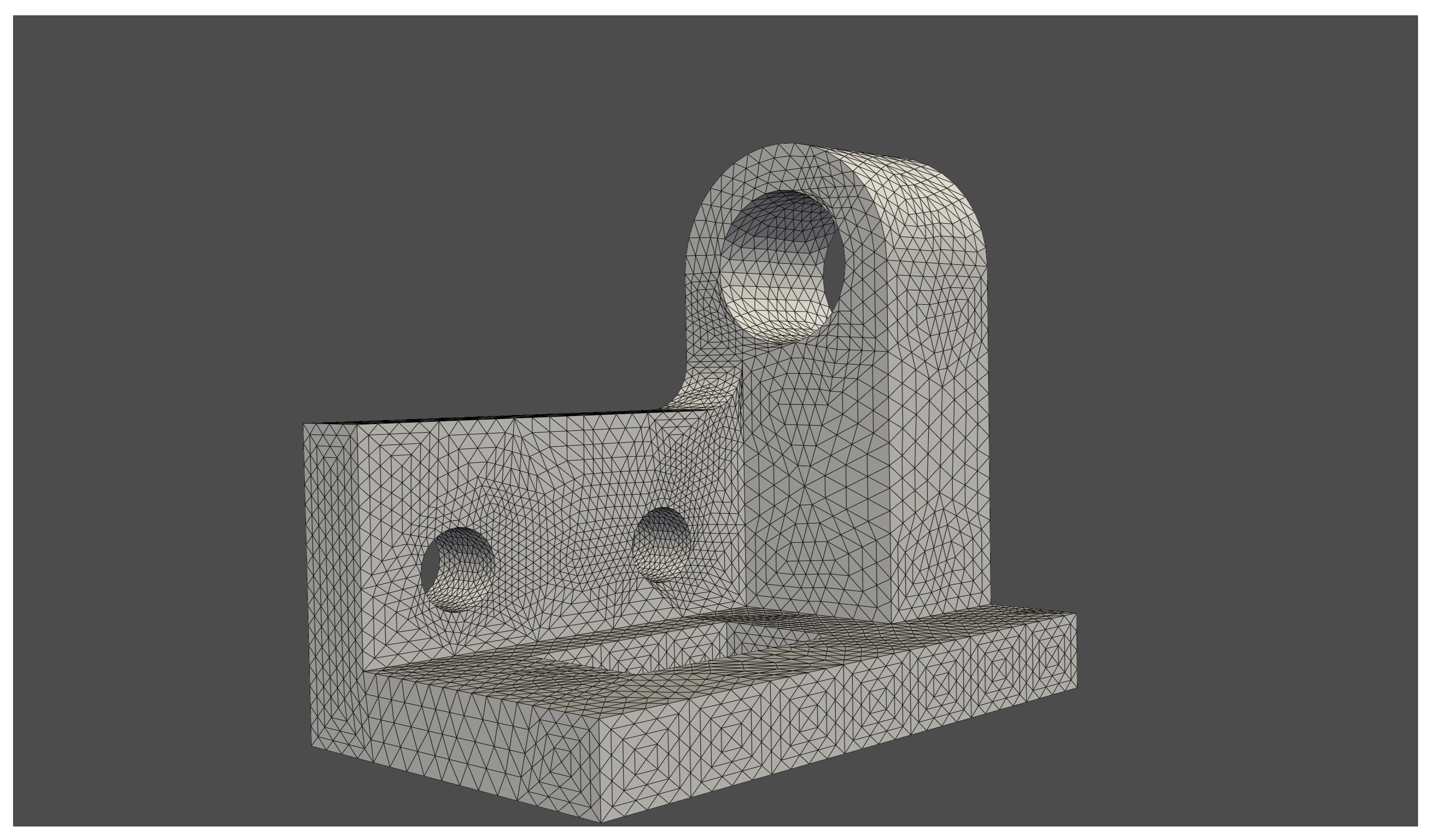
Convection is the transfer of heat between a solid and the surrounding fluid through conduction and fluid motion. It is governed by Newton’s law of cooling,

$${\dot{Q}}_{conv}=h{A}_s(T_s-T_{\infty }),$$

(7)

where h is the convection coefficient [26,27], $A_s$ is the area, $T_s$ is the surface temperature, and $T_{\infty }$ is the ambient temperature. Convection boundary conditions are Robin boundary conditions.

$$-\kappa \frac{\partial u}{\partial n}=r_0(u-s_0)on{\Gamma }_R^0,-\kappa \frac{\partial u}{\partial n}=r_1(u-s_1)on{\Gamma }_R^1,\cdots ,$$

(8)

where r is the convection coefficient and s is the surrounding ambient temperature.

3. Bracket Geometry

As mentioned in the introduction, the three-dimensional geometry of a bracket was made in Autodesk Inventor 2023. The geometry was then imported into Gmsh. The geometry was meshed and surface and volume facet tags were created to apply the required boundary conditions. The mesh has 86,592 elements and 15,603 nodes. The geometry used is shown in Figure 1 and Figure 2.

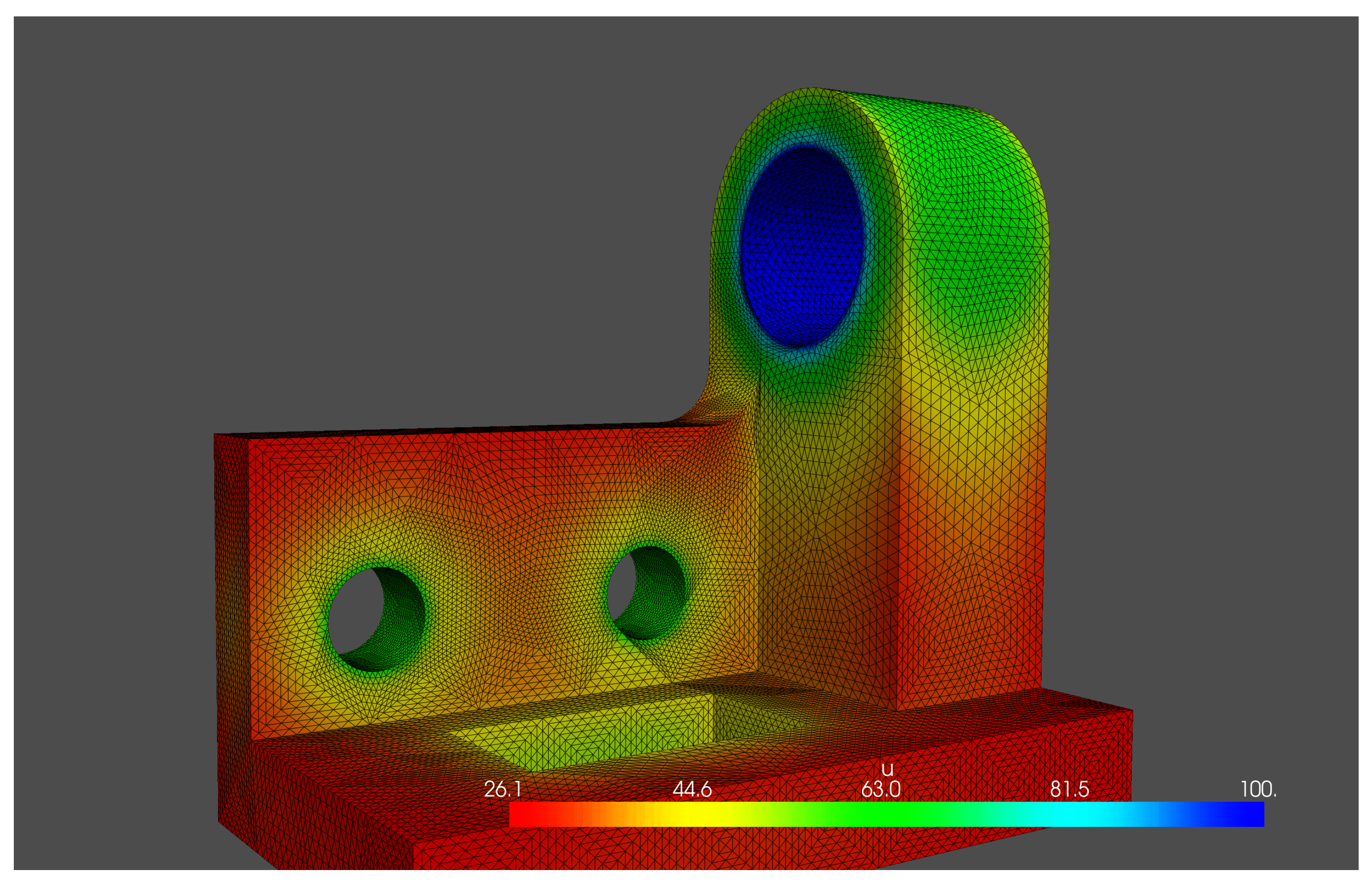
4. Steady Heat Conduction

Under steady state conditions, the time derivative on the RHS of Equation (3) is zero. Thus, the equation reduces to the Poisson equation:

$$\frac{{\partial }^{2}T}{\partial x^2}+\frac{{\partial }^{2}T}{\partial y^2}+\frac{{\partial }^{2}T}{\partial z^2}+\frac{{\dot{e}}_{gen}}{\kappa }=0.$$

(9)

It can also be represented as:

$$-\nabla ·(\kappa \nabla u)=-fin\Omega .$$

(10)

To solve this in FEniCSx, the PDE must be expressed in the variational form [28,29].

4.1. Variational Formulation

The variational form of Equation (10) is [30,31]:

$$-{\int }_{\Omega }\nabla ·(\kappa \nabla u)vdx={\int }_{\Omega }\kappa \nabla u·\nabla vdx-{\int }_{\partial \Omega }\kappa \frac{\partial u}{\partial n}vds.$$

(11)

To apply different BCs, the boundary integral is split into Neumann (Heat Flux) BCs and Robin (Convection) BCs:

$$-{\int }_{\partial \Omega }\kappa \frac{\partial u}{\partial n}vds=-\sum _i{\int }_{{\Gamma }_N^i}\kappa \frac{\partial u}{\partial n}ds-\sum _i{\int }_{{\Gamma }_R^i}\kappa \frac{\partial u}{\partial n}ds=\sum _i{\int }_{{\Gamma }_N^i}{g}_{i}ds+\sum _i{\int }_{{\Gamma }_R^i}{r}_i(u-s_i)ds.$$

(12)

Thus, we obtain the variational form as:

$$F={\int }_{\Omega }\kappa \nabla u·\nabla vdx+\sum _i{\int }_{{\Gamma }_N^i}{g}_{i}vds+\sum _i{\int }_{{\Gamma }_R^i}{r}_i(u-s_i)vds-{\int }_{\Omega }fvdx=0.$$

(13)

To obtain the bilinear and linear parts from Equation (13), the Robin BCs must be split:

$${\int }_{{\Gamma }_R^i}{r}_i(u-s_i)vds={\int }_{{\Gamma }_R^i}{r}_{i}uvds-{\int }_{{\Gamma }_R^i}{r}_i{s}_{i}vds.$$

(14)

Thus, the bilinear form is:

$$a(u,v)={\int }_{\Omega }\kappa \nabla u·\nabla vdx+\sum _i{\int }_{{\Gamma }_R^i}{r}_{i}uvds,$$

(15)

and the linear form is:

$$L\left(v\right)={\int }_{\Omega }fvdx-\sum _i{\int }_{{\Gamma }_N^i}{g}_{i}vds+\sum _i{\int }_{{\Gamma }_R^i}{r}_i{s}_{i}vds.$$

(16)

4.2. FEniCSx Implementation

All the simulations were run on a 13-inch MacBook Pro with 1.4 GHz quad-core Intel Core i5 with 128 MB eDRAM (Turbo Boost up to 3.9 GHz) and 8 GB of 2133 MHz LPDDR3 memory. The DOLFINx version used was 0.5.0. FEniCSx was installed using Conda as it is the recommended install method for Mac OS and is also available on Linux. The version of ParaView used was 5.10.1.

4.2.1. Importing the Mesh

The mesh along with the facet tags can be imported using the $read\_from\_mesh$ function from the dolfinx.io.gmshio library. The mesh file (mesh3D.msh) and the python script (SteadyThermal.py) must be in the same folder so that the script can access the mesh.

4.2.2. Defining the Function Space

After importing the mesh, the finite element function space has to be created. The most commonly used elements are Continuous Lagrange elements and the degree (order) of the function space can be varied as shown in Figure 3. Higher degree polynomial approximations provide superior results but take more time to solve [32,33]. This disadvantage is overcome by using a Krylov solver as it can speed up the execution of the program.

4.2.3. Defining the Variational Form and Boundary Conditions

The trial function u and test function v have to be defined before expressing the variational problem. To define the variational form, the boundary integral must be split into parts of Neumann and Robin BCs using the facet tags that are imported with the mesh. Facet tags are markers for different parts of the surface of the mesh. Tag 52 represents the large cylindrical hole, 53 represents the rectangular hole, 54 represents the two smaller cylindrical holes, and 55 represents the remaining surfaces. Facet tags are used to apply the BCs at the required boundary surface. The large cylindrical hole has a Dirichlet (constant temperature) condition of 100, the two smaller cylindrical holes have a Dirichlet condition of 60, the rectangular hole has a Neumann (heat flux) condition of 200 into the surface, and the rest of the surfaces have a Robin (convection) condition with r equal to 10. There is a heat generation of 10. After the creation of the boundary conditions, a For loop is run to collect all the Dirichlet boundary conditions in a list $bcs$ = [ ] and to append the boundary integral contributions to the variational form F.

4.2.4. Solving the Linear Variational Problem

The variational form F is split into the bilinear form $a(u,v)$ and linear form $L\left(v\right)$. The variational form is implemented into FEniCSx using the UFL library. The solution of the linear problem $u_h\in V$ is such that it satisfies $a(u,v)=L\left(v\right)$. PETSc is the linear algebra backend being used. The linear problem is solved using a preconditioned Krylov subspace method as it is much faster and requires 92% less memory than a direct solution [34]. The solution is stored as a XDMF file to be viewed in ParaView.

4.3. Results

The temperature contours for different orders are given below. Figure 4, Figure 5 and Figure 6 show the temperature contours for orders 1, 2, and 3 respectively. These plots were made using PyVista with ipygany as jupyter backend as it provides better contrasts. For higher order function spacess, PyVista joins the isoparametric nodes and makes the grid look more refined. The program was executed by running python SteadyThermal.py in the terminal.

The time taken for execution under direct and Krylov solvers for different orders of the function space is given in

Table 1. Comparison of execution time between direct and Krylov solvers for SteadyThermal.py.

Order	DOFs	Direct Solver	Krylov Solver(CG)
1	15,603	2.342662 s	1.241860 s
2	111,273	59.647889 s	2.411070 s
3	360,543	561.680618 s	9.031274 s
4	836,949	5047.619034 s	31.712334 s
5	1,614,027	45,448.596721 s	115.382458 s

.

As evident from Table 1, the number of DOFs increases drastically with the order of the function space. So the problem becomes much harder to solve with an increase in the order. The direct solver, LU factorization, is similar to Gaussian elimination. It is a very potent and simple method and can be efficiently used for many simpler problems with a few thousand unknowns. LU factorization solves the linear mesh with ease (2.34 s). However, sparse LU decomposition quickly becomes inefficient as the size of the matrix increases; it is very inefficient for order 2 (59.65 s) and struggles a lot for order 3 (561.68 s). On the other hand, the Krylov solver solves order 2 in 2.41 s (vs. 59.65 in direct solver) and order 3 in 9.03 s (vs. 561.68s in direct solver). Thus, the Krylov solver is far superior to the direct solver in terms of computational time. Since the result is the same as the one produced by the direct solver, there is no need to compare the results of the two solvers. Thus, the Krylov subspace solver is an iterative method that is faster and requires less memory. Figure 7 shows the bar chart of Time vs. Order for both direct and Krylov solvers. Note that the Time scale on the y-axis in Figure 7 is logarithmic.

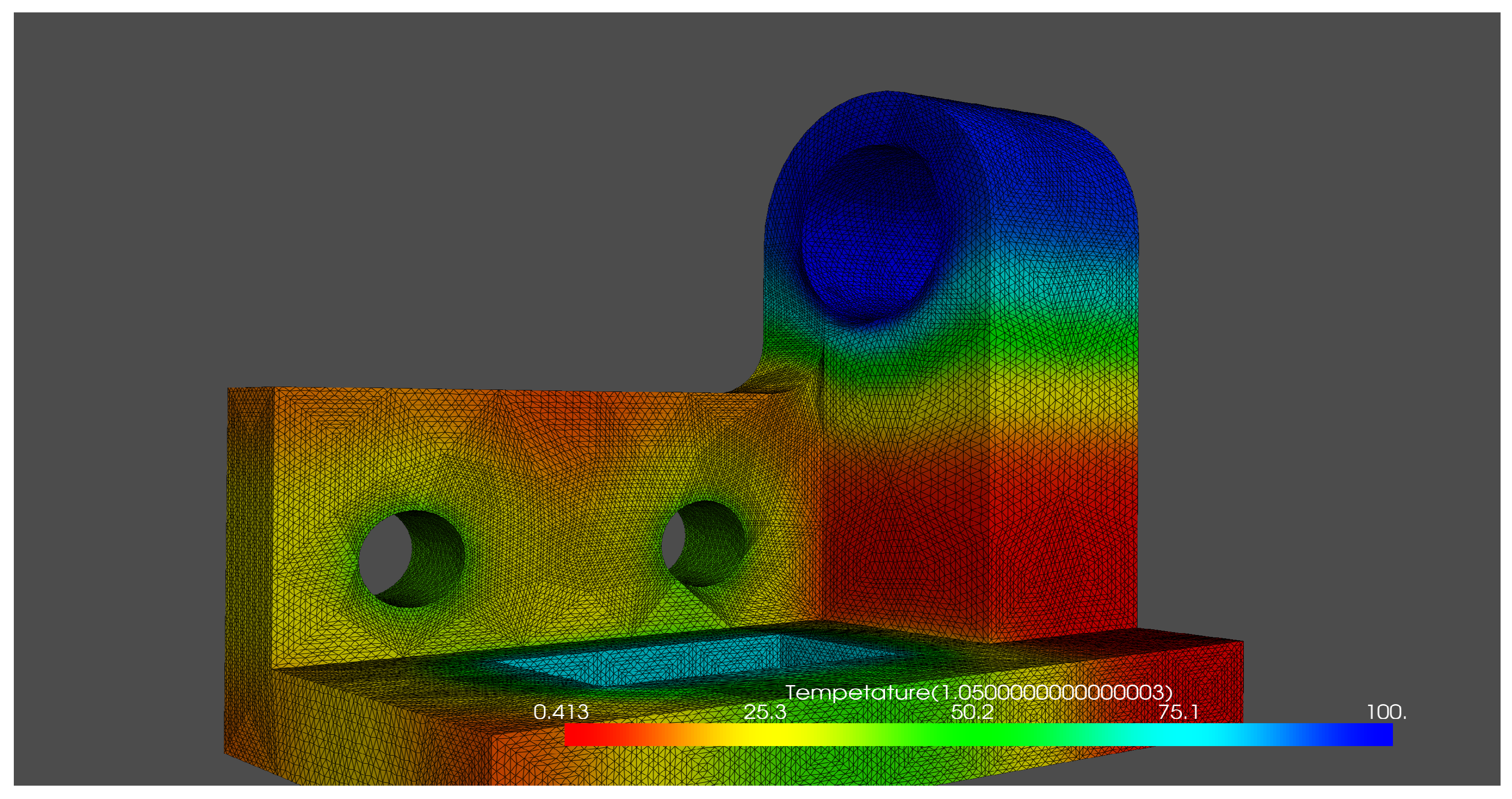
5. Transient Heat Conduction

Transient heat conduction is governed by Equation (3) and it can also be written as [28,29,35]:

$$\frac{\partial u}{\partial t}={\nabla }^{2}u+fin\Omega \times (0,T].$$

(17)

5.1. Variational Formulation

To solve time-dependent PDEs, the time derivative is discretized using a finite difference approximation:

$${\left(\frac{\partial u}{\partial t}\right)}^{n+1}={\nabla }^2{u}^{n+1}+f^{n+1}.$$

(18)

This reduces the problem to a sequence of stationary problems which then can be solved one after the other. The time-derivative can be approximated using a backward finite difference scheme:

$${\left(\frac{\partial u}{\partial t}\right)}^{n+1}\approx \frac{u^{n+1}-u^n}{\Delta t},$$

(19)

where $\Delta t$ is the time discretization parameter. Substituting Equation (19) in Equation (18) gives the time-discrete version of the transient heat equation called the implicit Euler discretization:

$$\frac{u^{n+1}-u^n}{\Delta t}={\nabla }^2{u}^{n+1}+f^{n+1}.$$

(20)

The above equation is rearranged in such a way that the right-hand side contains computed terms $u^n$ from the previous time step and the left-hand side contains the unknown $u^{n+1}$ in the current time step.

$$u^0=u_0,$$

(21)

$u_0$ is the initial conditions. Knowing $u_0$, solutions for $u^0$,$u^1$,$u^2$, and so on can be found:

$$u^{n+1}-\Delta t{\nabla }^2{u}^{n+1}=u^n+\Delta t{f}^{n+1},n=0,1,2,\dots$$

(22)

Equation (22) can also be written as:

$$u^{n+1}-\Delta t{\nabla }^2{u}^{n+1}-u^n-\Delta t{f}^{n+1}=0,n=0,1,2,\dots$$

(23)

The above equation is converted into the weak form by multiplying it with a test function v and integrating second-order derivatives by parts to give the bilinear form as:

$$a(u,v)={\int }_{\Omega }(uv+\Delta t\nabla u·\nabla v)dx,$$

(24)

and the linear form as:

$$L_{n+1}\left(v\right)={\int }_{\Omega }(u^n+\Delta t{f}^{n+1})vdx.$$

(25)

The variational form is implemented into FEniCSx using the UFL library.

5.2. FEniCSx Implementation

The transient heat conduction simulation was run on the same system as the steady conduction simulation. The DOLFINx version used is 0.5.0. The analysis was performed for HO function spaces using both the direct solver and the Krylov solver. In this transient analysis, the variational problem is solved 100 times, making it a much larger analysis to run compared to the steady-state analysis. Thus, the time for execution of this program is substantially larger than the steady state program. Importing the mesh and defining the function space is the same as the steady-state case given in Section 4.2. The variational problem is solved inside a For loop running from $t=0$ to $t=T$ with the time step dt. Thus the variational problem is solved for each time step and the result is stored in a XDMF file inside the loop.

5.2.1. Boundary Conditions

The large cylindrical hole has a Dirichlet BC of 100, the two smaller cylindrical holes have a Dirichlet BC of 40, the rectangular hole has a Dirichlet condition of 80, and the rest of the surfaces have a Neumann boundary condition of 0, i.e., an adiabatic or insulated boundary condition.

5.2.2. Temporal Parameters

The temporal parameters for this analysis are as follows:

• Start Time t = 0 s;
• Final Time T = 5 s;
• Step Size dt = 0.05 s;
• Number of time steps = T/dt = 100 steps.

5.3. Results

The temperature contours using a linear (order 1) function space at different time points are given below. Figure 8, Figure 9, Figure 10, Figure 11 and Figure 12 show the temperature distribution of the linear function space for t = 0.55, 1.05, 1.55, 2.55 and 4.55, respectively.

Figure 13, Figure 14 and Figure 15 show the temperature distribution of the cubic function space for t = 0.55, 1.05 and 4.05, respectively.

As mentioned before, these plots were made using PyVista with ipygany as the jupyter backend as it provides better contrasts. The program was executed by running python TransientThermal.py in the terminal. The results were exported in XDMF format and the animation can be viewed in ParaView.

The time taken for execution under direct and Krylov solvers for different orders of the function space is given in

Table 2. Comparison of execution time between direct and Krylov solvers for TransientThermal.py.

Order	DOFs	Direct Solver	Krylov Solver (CG)
1	15,603	80.71472 s	8.6550031 s
2	111,273	4803.45891 s	68.042709 s
3	360,543	21,769.80122 s	418.93187 s

.

As evident from the above table, the direct solver takes 80.7 s to solve order 1 while the Krylov subspace solver takes 8.65 s. Thus, the Krylov solver is around 9.3 times faster than the direct solver for the linear function space. The direct solver is very inefficient for HO function spaces and takes 1.33 h for order 2 and 6 h for order 3 as this analysis is far more computationally intensive than the steady-state analysis. The Krylov solver manages to produce results for HO function spaces in 68.04 s (vs. 1.3 h in direct solver) for order 2 and in 418.93 s (vs. 6 h in direct solver) for order 3. Thus, the Krylov subspace solver produces the same results in a much shorter time. Since the result is the same as the one produced by the direct solver, there is no need to compare the results of the two solvers.

6. Conclusions

This paper demonstrated steady and transient heat conduction in a three-dimensional bracket using the finite element method. Dirichlet, Neumann, and Robin BCs were used in the analysis. Since heat transfer happens almost everywhere, there are countless applications of FEM in solving thermal energy problems. Energy applications of heat conduction include engines, spacecraft, heat exchangers, electronic components, cooling systems, and chemical processes. In thermal engineering applications, the geometries of engines, turbochargers, radiators, and turbines are incredibly complex. The design of these machines requires accurate and reliable data from computational analysis about the temperature distribution and rate of heat flow as they are subjected to various thermal loads during operation [35,36]. Commercial packages such as ANSYS and ABAQUS can run standard simulations using already-established FEM frameworks. However, one cannot implement one’s formulations or run new solvers in commercial packages. Analysis using function spaces of order 3 and above with Krylov subspace solvers such as the ones presented in this paper is simply not possible in commercial packages. It is a well-established fact that using HO function spaces produces more accurate results while taking more time to solve. This disadvantage is overcome by using a preconditioned Krylov subspace method as it is much faster and requires 92% less memory than a direct solution. Thus, the methodology presented in this paper of combining HO function spaces with Krylov subspace solvers is superior in terms of both accuracy and speed. This opens the gateway to solving more complex problems that are yet to be solved. The time comparisons in Table 1 and Table 2 show that Krylov solvers can even be 30 times faster than a direct solver. The efficiency of the Krylov solvers allows one to perform complex and intensive simulations on personal computers reducing the necessity for expensive high-performance computers(HPCs). Another point to note is that, in the case of transient heat conduction, the solution of HO function space with a Krylov solver can be faster than the solution of linear function space with a direct solver. The BCs can easily be made time-dependent by making the values a function of time (ex: $100\ast {sin}^2(t-\pi )$). This provides a huge advantage over commercial FEM softwares as most commercial simulation softwares rely on direct solvers. FEniCSx makes it easy to enter the variational forms that are very close to the mathematical syntax and automates several features for anyone with a moderate level of knowledge of the mathematical framework of FEM. It is also an open-source package and is an excellent FEM tool for both learners and experts.

References

1. Kareem Jalghaf, H.; Omle, I.; Kovács, E. A Comparative Study of Explicit and Stable Time Integration Schemes for Heat Conduction in an Insulated Wall. Buildings 2022, 12, 824. [Google Scholar] [CrossRef]
2. Dokken, J.S.; Mitusch, S.K.; Funke, S.W. Automatic shape derivatives for transient PDEs in FEniCS and Firedrake. arXiv 2020, arXiv:2001.10058. [Google Scholar]
3. Cook, R.D.; Malkus, D.S.; Plesha, M.E.; Witt, R.J. Concepts and Applications of Finite Element Analysis; John Wiley & Sons, Inc.: Hoboken, NJ, USA, 2007. [Google Scholar]
4. Susanne, C.; Brenner, L. Ridgway Scott The Mathematical Theory of Finite Element Methods; Springer: New York, NY, USA, 2008. [Google Scholar] [CrossRef]
5. Smitha, T.V.; Nagaraja, K.V. An efficient automated higher-order finite element computation technique using parabolic arcs for planar and multiply-connected energy problems. Energy 2019, 183, 996–1011. [Google Scholar] [CrossRef]
6. Supriya, D.; Nagaraja, K.V.; Smitha, T.V.; Jayan, S. Accurate higher order automated unstructured triangular meshes for airfoil designs in aerospace applications using parabolic arcs. Aerosp. Sci. Technol. 2019, 88, 405–420. [Google Scholar]
7. Zhang, J.; Chauhan, S. Fast explicit dynamics finite element algorithm for transient heat transfer. Int. J. Therm. Sci. 2019, 139, 160–175. [Google Scholar] [CrossRef] [Green Version]
8. Bergagio, M.; Li, H.; Anglart, H. An iterative finite-element algorithm for solving two-dimensional nonlinear inverse heat conduction problems. Int. J. Heat Mass Transf. 2018, 126, 281–292. [Google Scholar] [CrossRef]
9. Kudela, L.; Chýlek, R.; Pospíšil, J. Efficient Integration of Machine Learning into District Heating Predictive Models. Energies 2020, 13, 6381. [Google Scholar] [CrossRef]
10. Luo, Y.; Zhang, L.; Feng, Y.; Zhao, Y. Three-Dimensional Streamline Tracing Method over Tetrahedral Domains. Energies 2020, 13, 6027. [Google Scholar] [CrossRef]
11. Alnaes, M.S.; Blechta, J.; Hake, J.; Johansson, A.; Kehlet, B.; Logg, A.; Richardson, C.; Ring, J.; Rognes, M.E.; Wells, G.N. The FEniCS Project Version 1.5. In Archive of Numerical Software 3; 2015; Available online: https://publications.lib.chalmers.se/records/fulltext/228672/local_228672.pdf (accessed on 1 October 2022).
12. Logg, A.; Mardal, K.A.; Wells, G. Automated Solution of Differential Equations by the Finite Element Method; Springer: Berlin/Heidelberg, Germany, 2012. [Google Scholar] [CrossRef]
13. Habera, M.; Hale, J.S.; Richardson, C.N.; Ring, J.; Rognes, M.E.; Sime, N.; Wells, G.N. FEniCSX: A sustainable future for the FEniCS project. In SIAM PP20 Minisymposium: Improving Productivity and Sustainability for Parallel Computing Software; Seattle, WA, USA, 2020; Available online: https://fenicsproject.org/citing/ (accessed on 1 October 2022).
14. Alnaes, M.S.; Logg, A.; Ølgaard, K.B.; Rognes, M.E.; Wells, G.N. Unified Form Language: A domain-specific language for weak formulations of partial differential equations. ACM Trans. Math. Softw. 2014, 40, 1–37. [Google Scholar] [CrossRef]
15. Scroggs, M.W.; Dokken, J.S.; Richardson, C.N.; Wells, G.N. Construction of arbitrary order finite element degree-of-freedom maps on polygonal and polyhedral cell meshes. ACM Trans. Math. Softw. 2022, 48, 1–23. [Google Scholar] [CrossRef]
16. Scroggs, M.W.; Baratta, I.A.; Richardson, C.N.; Wells, G.N. Basix: A runtime finite element basis evaluation library. J. Open Source Softw. 2022, 7, 3982. [Google Scholar] [CrossRef]
17. Kirby, R.C.; Logg, A. A compiler for variational forms. ACM Trans. Math. Softw. 2006, 32, 417–444. [Google Scholar] [CrossRef] [Green Version]
18. Geuzaine, C.; Remacle, J.-F. Gmsh: A three-dimensional finite element mesh generator with built-in pre- and post-processing facilities. Int. J. Numer. Methods Eng. 2009, 79, 1309–1331. [Google Scholar] [CrossRef]
19. Sullivan, C.; Kaszynski, A. PyVista: 3D plotting and mesh analysis through a streamlined interface for the Visualization Toolkit (VTK). J. Open Source Softw. 2019, 4, 1450. [Google Scholar] [CrossRef]
20. Ahrens, J.; Geveci, B.; Law, C. ParaView: An End-User Tool for Large Data Visualization. In Visualization Handbook; Elsevier: Amsterdam, The Netherlands, 2005; ISBN -13: 978-0123875822. [Google Scholar]
21. Ayachit, U. The ParaView Guide: A Parallel Visualization Application; Kitware: New York, NY, USA, 2015; ISBN 978-1930934306. [Google Scholar]
22. Van Der Vorst, H.A. Krylov Subspace Iteration. Comput. Sci. Eng. 2000, 2, 32–37. [Google Scholar] [CrossRef]
23. Gao, C.; Liu, Y.; You, R.; Li, H. Theoretical and Numerical Study on Thermal Insulation Performance of Thermal Barrier Coatings. Energies 2022, 15, 6880. [Google Scholar] [CrossRef]
24. Moumtzakis, A.; Zoras, S.; Evagelopoulos, V.; Dimoudi, A. Experimental Investigation of Thermal Bridges and Heat Transfer through Window Frame Elements at Achieving Energy Saving. Energies 2022, 15, 5055. [Google Scholar] [CrossRef]
25. Cengel, Y.A.; Ghajar, A.J. Heat and Mass Transfer: Fundamentals and Applications, 6th ed.; McGraw-Hill Professional: New York, NY, USA, 2020. [Google Scholar]
26. Piasecka, M.; Maciejewska, B.; Łabędzki, P. Heat Transfer Coefficient Determination during FC-72 Flow in a Minichannel Heat Sink Using the Trefftz Functions and ADINA Software. Energies 2020, 13, 6647. [Google Scholar] [CrossRef]
27. He, J.; Wang, K.; Li, J. Numerical Analysis of the Convective Heat Transfer Coefficient Enhancement of a Pyro-Breaker Utilized in Superconducting Fusion Facilities. Energies 2021, 14, 7565. [Google Scholar] [CrossRef]
28. Langtangen, H.P.; Logg, A. Solving PDEs in Python The FEniCS Tutorial I; Springer: Cham, Switzerland, 2016. [Google Scholar] [CrossRef]
29. Reddy, J.N.; Gartling, D.K. The Finite Element Method in Heat Transfer and Fluid Dynamics; CRC Press: Boca Raton, FL, USA, 2011. [Google Scholar] [CrossRef]
30. Langtangen, H.P.; Mardal, K.-A. Introduction to Numerical Methods for Variational Problems; Springer: Cham, Switzerland, 2016. [Google Scholar] [CrossRef]
31. Larson, M.G.; Bengzon, F. The Finite Element Method:Theory, Implementation, and Applications. In Texts in Computational Science and Engineering; Springer: Berlin/Heidelberg, Germany, 2013. [Google Scholar] [CrossRef]
32. Smitha, T.V.; Nagaraja, K.V. Application of automated cubic-order mesh generation for efficient energy transfer using parabolic arcs for microwave problems. Energy 2019, 168, 1104–1108. [Google Scholar] [CrossRef]
33. Kumar, S.; Jakkareddy, P.S.; Balaji, C. A novel method to detect hot spots and estimate strengths of discrete heat sources using liquid crystal thermography. Int. J. Therm. Sci. 2020, 154, 106377. [Google Scholar] [CrossRef]
34. McDonagh, J.; Palumbo, N.; Cherukunnath, N.; Dimov, N.; Yousif, N. Modelling a permanent magnet synchronous motor in FEniCSx for parallel high-performance simulations. Finite Elem. Anal. Des. 2022, 204, 103755. [Google Scholar] [CrossRef]
35. Singh, P. Errors Incurred in Local Convective Heat Transfer Coefficients Obtained through Transient One-Dimensional Semi-Infinite Conduction Modeling: A Computational Heat Transfer Study. Energies 2022, 15, 7001. [Google Scholar] [CrossRef]
36. Jakkareddy, P.S.; Balaji, C. Estimation of local heat transfer coefficient from natural convection experiments using liquid crystal thermography and Bayesian method. Exp. Therm. Fluid Sci. 2018, 97, 458–467. [Google Scholar] [CrossRef]
Figure 1. Bracket geometry with tetrahedron meshing.
Energies 15 08077 g001
Figure 2. Overhead view of the bracket geometry.
Energies 15 08077 g002
Figure 3. Continuous Lagrange tetrahedron for order = 1, 2, 3, 4, 5, 6.
Energies 15 08077 g003
Figure 4. Temperature contour of a function space of order 1.
Energies 15 08077 g004
Figure 5. Temperature contour of a function space of order 2.
Energies 15 08077 g005
Figure 6. Temperature contour of a function space of order 3.
Energies 15 08077 g006
Figure 7. Comparison of execution time between direct and Krylov solvers.
Energies 15 08077 g007
Figure 8. Temperature contour of a function space of order 1 at t = 0.55 s.
Energies 15 08077 g008
Figure 9. Temperature contour of a function space of order 1 at t = 1.05 s.
Energies 15 08077 g009
Figure 10. Temperature contour of a function space of order 1 at t = 1.55 s.
Energies 15 08077 g010
Figure 11. Temperature contour of a function space of order 1 at t = 2.55 s.
Energies 15 08077 g011
Figure 12. Temperature contour of a function space of order 1 at t = 4.55 s.
Energies 15 08077 g012
Figure 13. Temperature contour of a function space of order 3 at t = 0.55 s.
Energies 15 08077 g013
Figure 14. Temperature contour of a function space of order 3 at t = 1.05 s.
Energies 15 08077 g014
Figure 15. Temperature contour of a function space of order 3 at t = 4.05 s.
Energies 15 08077 g015