Article

Numerical Study of the Impact of Fluid–Structure Interaction on Flow Noise over a Rectangular Cavity

Department of Power Systems and Environmental Protection Facilities, Faculty of Mechanical Engineering and Robotics, AGH University of Science and Technology, Mickiewicz 30 av, 30-059 Kraków, Poland
*
Author to whom correspondence should be addressed.
These authors contributed equally to this work.
Energies 2022, 15(21), 8017; https://doi.org/10.3390/en15218017
Submission received: 21 September 2022 / Revised: 7 October 2022 / Accepted: 13 October 2022 / Published: 28 October 2022

Abstract

:
Fluid–structure interactions (FSI) can significantly affect flow and the acoustic field generated by it. In this article, simulations of the flow over a rectangular cavity are conducted with and without taking FSI into account. The aim of this research is to conduct a numerical study of the flow over a cavity and to verify whether interactions between the flow and the elastic structure can significantly affect the flow itself or the acoustic pressure field. Four cases involving flexible walls with different material parameters and one reference case with rigid walls were analysed. The two-directional fluid–structure coupling between the flow and cavity walls was simulated. The simulations were performed with the volume and finite element methods using OpenFOAM software to solve the fluid field, CalculiX software to solve the displacement of the structure, and the preCICE library to couple the codes and computed fields. The acoustic analogy of Ffowcs-Williams and Hawkings and the libAcoustics library were used to calculate the sound pressure. The simulation results showed that FSI has a significant influence on sound pressure in terms of both pressure amplitudes and levels as well as in terms of noise frequency composition. There was a significant increase in the sound pressure compared to the case with rigid walls, especially for frequencies above 1 kHz. The frequencies at which this occurred are related to the natural frequencies of the cavity walls and the Rossiter frequencies. Overlap of these frequencies may lead to an increase in noise and structural vibrations, which was observed for one of the materials used. This study may provide insight into the flow noise generation mechanism when fluid–structure interactions are taken into account. The conclusions presented here can form a basis for further work on aerodynamic noise in the presence of thin-walled structures.

1. Introduction

Flow over a cavity is widely used as a model of flow over discontinuities, even ones with complex-shape. Historically, this research object arose from the problem of noise generated by aircraft weapon bays [1] and landing gear. A cavity is used as a model to describe flow phenomena and noise generation by car mirrors and door cavities [2], pantographs, recesses on the roofs of trains [3], and other vehicle discontinuities. Cavities are often used to analyse the flow in different parts of ventilation ducts. This was the goal of Radavich [4], who investigated the flow inside quarter-wave resonators, and of Lafon [5], who identified the tones in gate valves inside a duct.
The flow over a cavity has been widely investigated in the past via theoretical, numerical, and experimental techniques due to the complex phenomena involved, such as vortex shedding, free shear layer instability, and pressure oscillations. Rossiter [6], in his experimental study, was one of the first to attempt to derive the dependence describing the pressure fluctuations occurring in cavities. Under certain conditions, the flow past cavities starts to oscillate in a self-sustaining manner. Rockwell [7] describes three different types of self-sustaining oscillations of flow: fluid dynamic, fluid resonant, and fluid elastic. Most of the works dealing with cavity flow and noise focuses on fluid dynamic and fluid resonant oscillations, ignoring the effect of flexible cavity walls on the flow over the cavity and the aeroacoustic feedback it generates. There are only few studies on the third type of interaction, fluid elastic; these are mostly limited to unidirectional fluid–structure coupling, and assume that the vibrating structure has no influence on the flow. Yokohama [8] researched the impact of flow on the vibrations of a flexible cantilever beam attached to the upstream and downstream edges of a cavity. Thangamani [9] investigated the possible ways to harvest energy from flow by attaching a flexible piezoelectric beam at the downstream wall.
There are studies in which bidirectional fluid–structure coupling has been analysed. However, these are usually limited to the simplified case of a lid-driven cavity, which is a well known benchmark case for CFD. This model involves solving only the flow within the cavity, with the flow over the cavity replaced by appropriate boundary conditions. Khanafer [10] examined the effect of a heated flexible cavity bottom on heat transfer in such a system. Alsabery [11] researched a similar problem involving heat transfer in a lid-driven cavity with elastic walls and with a hot rotating cylinder in the middle of the cavity. Sun [12] analysed the vibrations of the lid-driven cavity walls themselves under flow in terms of the dependence of the rigidity and Reynolds number. Sabbar [13] investigated the flow over a cavity with a downstream flexible wall at a low Reynolds number and with a heat source at the bottom of the cavity. Most of the above works describing the fluid–structure interactions ocurring in cavities are modeled and solved numerically, and are limited only to the case of a lid-driven cavity. There is very little research focusing on the FSI effects ocurring in cavities placed in channels or open spaces. Moreover, the most common consideration of flexible walls is to increase heat transfer, while the research largely ignores their impact on the noise generated by the flow.
In the present work, we investigate fluid elastic oscillations and analyse their impact on the noise generated by the flow over a cavity. The length L to depth D ratio is used to describe the type of cavity. The flow over a cavity with an L / D ratio of 4 was analysed along with the vibrations of the cavity walls. The main assumption of this study was to model a cavity inside a ventilation duct. Hence, the thickness of elastic cavity walls was similar to the thickness of typical duct walls. We used four different sets of material parameters to model the different flexible walls of the cavity and one model with rigid walls as a reference model. The adopted materials were typical materials for making ventilation ducts. The flow velocities were typical of those found in the ducts. To the best of our knowledge, such research on the fluid–structure interactions cavity flow has not yet been performed. There are no numerical studies taking into account the influence of the structural vibrations generated by the flow on the aeroacoustic noise in the case of flow over a cavity.
To investigate this phenomenon, finite volume and finite element methods were used. We used the detached eddy simulation method described by Strelets [14] with the k ω SST model developed by Menter [15] to compute the flow over the cavity. Typically, the large-eddy simulation model is used for hybrid flow acoustics simulations [16]. However, a model combining the LES and RANS models, namely, the DES model, is now used more often in this type of simulation [17,18] as well as in cavity noise problems [19]. We chose the k ω SST DES model due to the fact that it combines the high accuracy of the LES model with the high computational speed of the RANS model. To model the fluid-induced vibrations, it was first necessary to solve the dynamics of the cavity walls. This was carried out using the classical finite element method. The bidirectional coupling between the flow and displacement fields was modeled. The values of forces exerted on the walls by the fluid and nodal displacement of the structure were exchanged. The preCICE library [20] was used to couple the fields and model the fluid–structure interaction.
The main objective of the study was to compute the acoustic pressure generated by the flow. The acoustic analogy of Lighthill [21] and its extension provided by Ffowcs-Williams and Hawkings [22] were used to achieve this. We used the hybrid CFD-CAA method to compute the noise based on the fluid flow simulation results. This approach combines two-way fluid–structure coupling with the use of acoustic analogies, and has been successfully used in the analysis of aeroacoustic and hydroacoustic noise [23] and in case of forced oscillations of a cylinder in flow [24]. The computational model itself was verified and compared with experimental results by Turek and Hron [25] in the study conducted by Chourdakis et al. [26]. The presented research is a continuation and summary of the preliminary analyzes presented in [27].
This study is important due to the possible consequences of taking into account flexible walls in the flow, especially when analysing noise in thin-walled systems. Additionally, this type of analysis can provide information on possible energy recovery of flows over cavities when flow-induced vibrations are taken into account. This type of work has already been carried out by Thangamani [9]; however, as mentioned earlier, the influence of the vibrating structure on the flow itself was ignored. Moreover, this problem can be developed towards possible damping of vibrations and noise in cavities by placing additional elastic vibrating structures in them, as shown in [28,29].
In addition, the findings of this study can be used in other industries where flows over cavities occur, primarily aviation and high-velocity rail transport. In addition, the observations made in this work can be used in analyses of the noise generated by flows in the presence of thin-walled systems more generally, not necessarily cavities/ducts.
The outline of this paper is as follows. In Section 2, the mathematical models of flow and structural vibrations are described along with the numerical methods used to solve them. In Section 3, the analysed model, simulation initial and boundary conditions, and grid independence study are presented. The results of simulations involving the acoustic pressure at the receiver, forces acting on the cavity, and flow fields are described and analysed in Section 4. Finally, the main findings and conclusions are provided in Section 5.

2. Mathematical Model and Numerical Methods

2.1. Flow Modeling

In this study, turbulent fluid motion was described by the k ω SST DES (Detached Eddy Simulation) model [14]. This model solves RANS (Reynolds-Averaged Navier–Stokes) equations with the k ω SST turbulence model in the boundary layer and LES (Large Eddy Simulation) in the separated region. The incompressible form of RANS equations were used for relatively low flow velocities, i.e., those for which the Mach number is much smaller than unity. The RANS continuity and momentum equations are provided by (1) and (2) [30]:
v ¯ i x i = 0
ρ v ¯ i t + ρ v ¯ j v ¯ i x j = p ¯ x i + x j τ ¯ i j ρ v i v j ¯
where v i = v ¯ + v i is the i-th component of the velocity, i = x , y , z in the Cartesian coordinate system, p = p ¯ + p is the pressure, ρ is the density, τ ¯ i j is the laminar viscous stress tensor, and ρ v i v j ¯ = τ i j R is the Reynolds stress tensor. In the above equation, a bar denotes an averaged component and prime denotes a fluctuating component, unless stated otherwise.
The Bousinessq hypothesis introduced the concept of eddy viscosity μ t (3), which allows the Reynolds stress tensor to be modeled by means of turbulence models.
τ i j R = 2 μ t S i j 1 3 u k x k δ i j 2 3 k δ i j
In this work, we have chosen the k ω SST model as suitable for aerodynamics [15]. In this model, two equations are solved: one for turbulent kinetic energy k (4), and one for the specific turbulent dissipation rate ω (5):
D ρ k D t = τ i j u i x j β * ρ ω k + x j μ + σ k μ t k x j
D ρ ω D t = γ ν t τ i j u i x j β ρ ω 2 + x j μ + σ ω μ t ω x j + 2 ρ 1 F 1 σ ω 2 1 ω k x j ω x j
where D D t = t + u i x i is the material derivative, k is the turbulent kinetic energy, ω is the specific turbulent dissipation rate, β * , σ k σ ω , γ , a 1 are model constants, and F 1 , F 2 are additional functions.
The model is described in greater detail in [15]. The turbulent eddy viscosity is then computed with
μ t = ρ a 1 k max ( a 1 ω , S F 2 )
The LES continuity and momentum equations are provided by (7) and (8) [30]. In this kind of simulation, the flow is not decomposed by Reynolds averaging, as before, but by spatial filtering into the filtered ϕ ¯ and sub-filtered ϕ parts:
v ¯ i x i = 0
v ¯ i t + x j v ¯ i v ¯ j = 1 ρ p ¯ x i + x j τ i j S + 2 ν S ¯ i j
where τ i j S = u ¯ i u ¯ j u i u j ¯ is the subgrid-scale (SGS) stress tensor.
This SGS stress tensor has to be modeled, and in case of k ω SST DES, the k ω SST model is used as a subgrid-scale model. The switching between LES and RANS is based on the values of the maximum spatial step Δ and the length scale l ˜ , which are defined by Strelets [14]. If the length scale is less than C D E S Δ , then the k ω SST model is used; otherwise, the LES equations are solved for mesh cells with δ x , δ y , and δ z dimensions:
Δ = max ( δ x , δ y , δ z )
l ˜ = min ( l k ω , C D E S Δ )
OpenFOAM v.2012 was used to perform the fluid flow simulations. OpenFOAM is an open-source CFD software that uses the finite-volume method [31]. Because of its robustness, the PIMPLE algorithm [32], which combines SIMPLE (Semi-Implicit Method for Pressure Linked Equations) [33] and PISO (Pressure-Implicit with Splitting of Operators) [34], was used to solve the equations of the flow field. The SIMPLE algorithm was used to determine the initial conditions in the computational domain based on boundary conditions. To compute the gradient and divergence terms, the upwind and standard linear Gauss methods were used.

2.2. Structural Modeling

The motion of the structural part of the model, that is, the cavity walls, was described by the general momentum equation from structural analysis without damping terms [35]:
[ M ] { U ¨ } + [ K ] { U } = { F }
where { U ¨ } = { A } is the global acceleration vector, { U } is the global displacement vector, [ M ] is the global mass matrix, [ K ] is the global stiffness matrix, and { F } is the global force vector.
The damping terms was not taken into account, as the simple dynamic model and the lack of additional coefficients were assumed. This equation is discretized in space by they finite element method and in time by finite differences. It is solved using the α -method, which is an extension of the Newmark method [35].
Equation (11) is discretized in space by the finite element method. The local (element) stiffness and mass matrices are provided by [35]
K e ( i K ) ( j M ) = V 0 e φ i , L Σ K L M N ( θ ) φ j , N d V e
M e ( i K ) ( j M ) = V 0 e ρ 0 φ i φ j d V e
F e ( i K ) = A O e T ¯ ( N ) k φ i d A e + V 0 e ρ 0 f k φ i d V e + V 0 e β K L θ T γ K L φ i , L d V e
where Σ K L M N is the free energy function, K L M N are the material coordinates, θ is the absolute temperature, ρ 0 is the mass density, T ¯ K is the traction, f k is the force per unit mass, β K L is the thermal stress tensor per unit temperature, γ K L is the residual stress tensor, and φ represents the shape functions.
After Equation (11) is discretized in time, it takes the form
M A n + 1 + K U n + 1 = F n + 1 e x t
A n + 1 = A n + Δ A
U n + 1 = U n + Δ t V n + 1 + 1 2 Δ t 2 1 2 β A n + 2 β A n + 1
where the subscript n denotes the current and n + 1 the next time step.
The algorithm is second order accurate and unconditionally stable for α 1 3 , 0 [35]. The parameter β is provided by
β = 1 4 1 α 2
In this study, we used an eight-node brick element, which is a general-purpose fully integrated brick element, sometimes called a linear brick element. The shape functions of this element are provided by [36]:
φ = 1 8 1 + ξ ξ i 1 + η η i 1 + ζ ζ i i = 1 , 2 , , 8
where ξ i , η i , ζ i are the local coordinates of the th point. Very small thickness of the walls of the cavity and the ventilation duct encouraged the use of shell elements, however this turned out to be impossible due to the limitations of the preCICE library.
The structural modeling was performed using CalculiX open source finite element sofware [35].

2.3. Coupling of the Fields

As mentioned before, the coupling between the fluid flow field, computed with OpenFOAM and the solid displacement field computed with CalculiX was carried out using the preCICE coupling library. preCICE allows both explicit and implicit methods for solving interface equations and data mapping between different physical fields and computational meshes. In addition, it allows for communication between different codes, not only OpenFOAM and CalculiX [20].
In this study, we used the serial explicit coupling scheme. This scheme uses the nth timestep values x 1 ( n ) of a solver S 1 as boundary values for the n + 1 time step value of a solver S 2 and solution x 2 ( n + 1 ) , then uses the result for computation of x 1 ( n + 1 ) . Nearest-neighbor and nearest-projection methods were used for data mapping between fields. These were chosen due to the simplicity of their working principles and the fact that the size of the interface edges is similar. As mentioned before, bidirectional fluid–structure interaction was modeled. The displacement and force fields had to be exchanged between solvers. The forces exerted by the fluid on the walls are the boundary conditions (loads) for the structure simulation. A displacement field is obtained from them, then transferred to the fluid calculations as the mesh displacement [25].

2.4. Aeroacoustics

The noise generated by the flow over the cavity and the oscillations of the cavity walls was computed by means of acoustic analogies. The acoustic analogy determines how the sound caused by the flow would propagate in unlimited and undisturbed domain without the flow. As the Lighthill acoustic analogy assumes that there are no walls to disrupt the flow, it was impossible to use it directly [21]. Therefore, in this work, the Ffowcs-Williams and Hawkings (FWH) acoustic analogy was used. It allows the noise generated by the flow in the vicinity of the moving walls to be calculated [22]. The FWH analogy equation is provided by [37]:
2 ρ H s t 2 c 2 2 ρ H s x i 2 = 2 T i j H s x i x j x i ρ v i v j V j + p i j n j δ f f + t ρ v j ρ V j n j δ f f
where ρ repesents the (acoustic) density fluctuations, H s is the Heaviside step function, T i j = ρ v i v j + ( p p ) ( ρ ρ ) c 2 δ i j σ i j is the Lighthill stress tensor, c is the speed of sound, V i is the velocity of the surface in direction i, f is the scalar function defining the surface, and δ is the Dirac delta function.
We used the solution of this equation derived by Brentner and Farassat by means of generalized functions [38], called Formulation 1A:
p ( x , t ) = p T ( x , t ) + p L ( x , t ) ,
4 π p t ( x , t ) = f = 0 ρ 0 v ˙ n + v n ˙ r 1 M r 2 ret d S + f = 0 ρ 0 v n r M ˙ r + c M r c M 2 r 2 1 M r 3 ret d S ,
4 π p L ( x , t ) = 1 c f = 0 l ˙ r r 1 M r 2 r e t d S + f = 0 l r l M r 1 M r 2 ret d S   + 1 c f = 0 l r M ˙ r + c M r c M 2 r 2 1 M r 3 ret d S .
where ϕ n is the dot product of variable ϕ with a unit normal vector, ϕ r is the dot product of ϕ with a radiation vector, ϕ M is the dot product of ϕ with a normalized surface velocity vector, ϕ r e t is the quantity evaluated at the retarded time τ = t r c , r is the distance between the observer and source, l is the local force acting on the surface, and ϕ ˙ = ϕ τ is the source time derivative of ϕ .
The Equations (21)–(23) were implemented and solved in OpenFOAM software with the libAcoustics library [39].

3. Case Description

3.1. Computational Domain

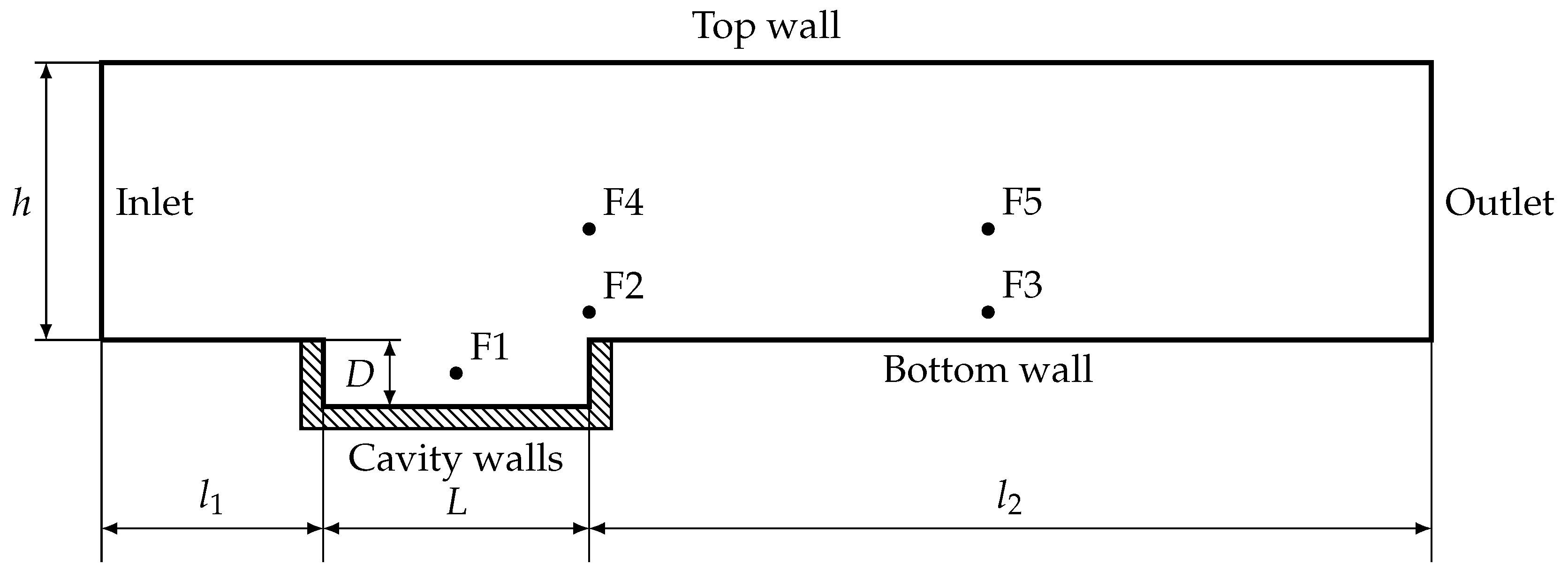
The computational domain used in our analyses is shown in Figure 1. It is defined as a section of a rectangular ventilation duct with a cavity at its bottom. The ratio of cavity length to depth L / D was equal to 4 in all simulations; therefore, the analysed cavity can be classified as a shallow cavity ( L / D > 1 ) [40]. The length of the cavity itself was chosen to represent a possible junction of the channel that has been closed. The length of the domain upstream and downstream of the cavity allows the dynamic phenomena occurring in the cavity to be captured, including vortex shedding, shear layer instabilities, and separation of the flow. The dimensions of the domain are presented in Table 1. They are based on the dimensions of a ventilation duct with a square cross-section with a depth equal to 0.125 m.
The computational mesh was generated based on the computational domain described above. The fluid mesh was generated using cfMesh and the structural mesh using GMSH open-source meshing tools. Based on the grid independence study described later in the article, fluid mesh #3, described in Table 2, and structural mesh #3, described in Table 3, were selected for all simulations.

3.2. Initial and Boundary Conditions

The boundaries of the fluid computational domain are shown in Figure 1. On each of them, the boundary conditions for each variable to be solved had to be set. The boundary conditions for the turbulent kinetic energy k and specific dissipation rate ω were estimated based on the recommendations of the author of the k ω SST turbulence model [15]. The boundary conditions for each of the variables are shown in Table 4. Because of the implementation of the incompressible flow model in OpenFOAM, the pressure shown in the table and used for computations was scaled by density.
Moreover, the cavity walls, which acted as the interface between the fluid flow and structural simulations, were flexible and able to move. The wall movement was determined based on structural simulations.
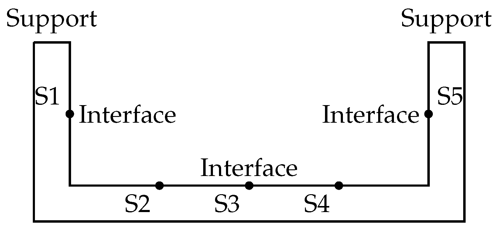
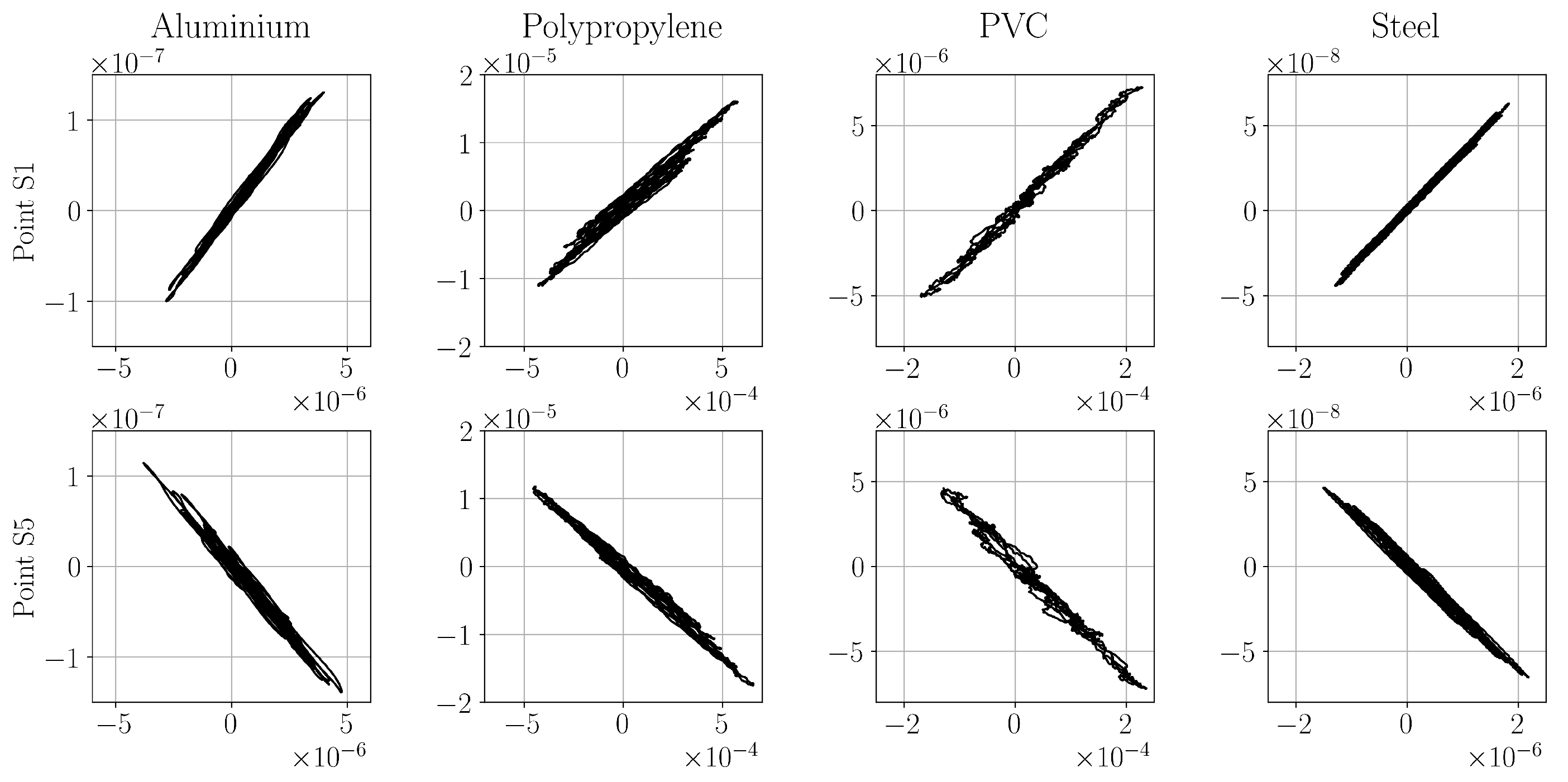
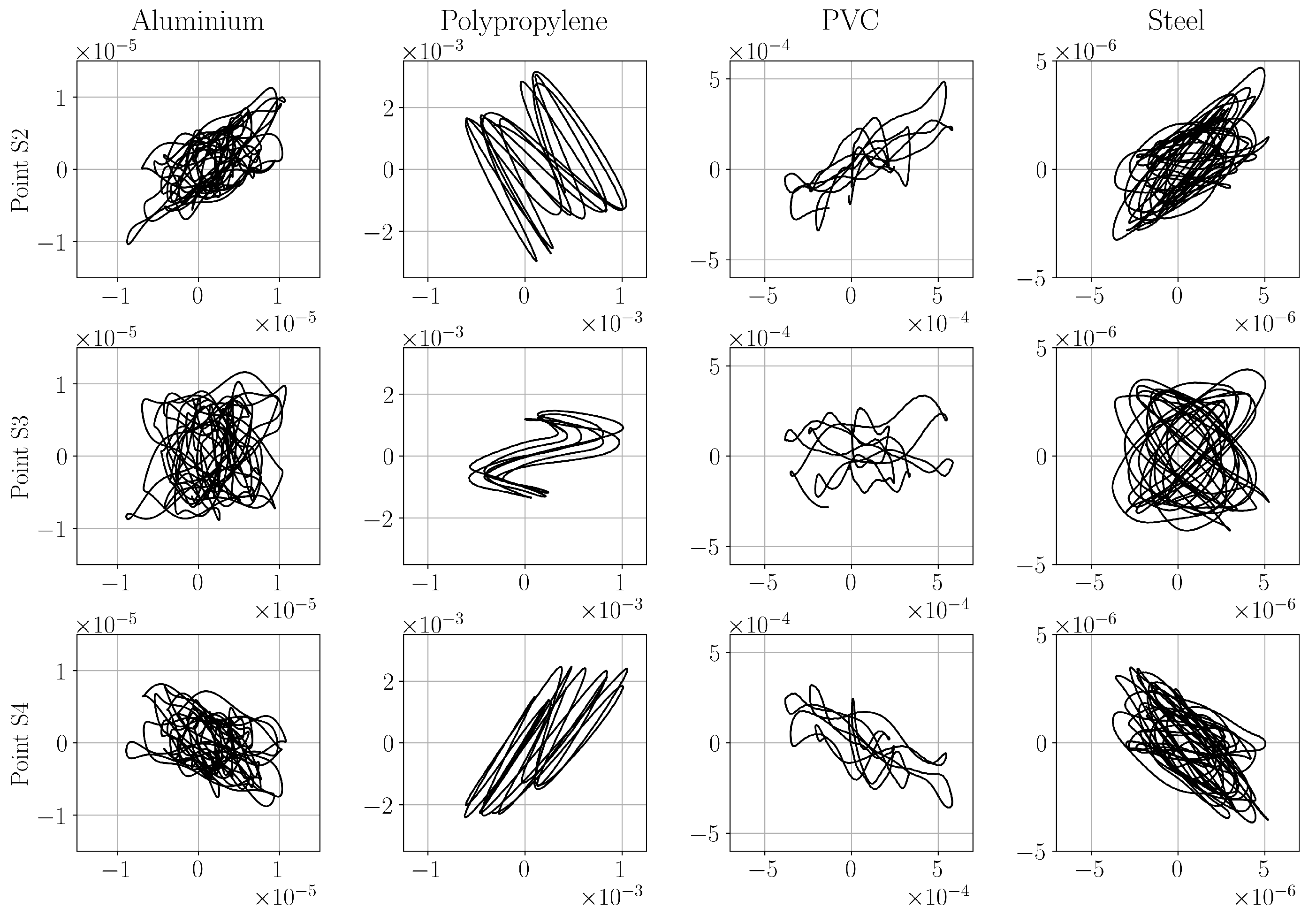
The boundaries of the computational domain for structural simulations are shown in Figure 2. The same figure shows the probes where the displacement was recorded. At the boundary denoted Support, all degrees of freedom were constrained from movement in each direction. The boundary denoted Interface acted as a coupling surface between the fluid and structural simulations. In the case of structural analyses, it was the surface where the force from the fluid flow simulations was applied.

Material Parameters

Table 5 shows the parameters of the chosen materials, which are generally used for ventilation channels and ducts [41]. These materials were used for modeling the structural simulations. An air temperature of 20 °C, density ρ = 1.23   kg / m 3 , kinematic viscosity 1.5 × 10 5   m 2 / s , and speed of sound c = 340 m/s were selected for the flow simulations.

3.3. Grid Independence Study

Two grid independence studies were performed, one for the fluid mesh and the other for the structural mesh. The main evaluation criteria for both studies were the sound pressure level evaluated at selected receivers using the FWH acoustic analogy, given by Equation (21) and the displacement of a point placed at the bottom of the cavity wall, computed from structural analyses. In addition, the simulation time and the values of the y + parameter (defined as a dimensionless distance from the wall) were checked and compared. In order to properly resolve the boundary layer and viscous sublayer, the values of y + should be less than unity. In all independence studies (both finite volume and finite element mesh), the timestep of Δ t = 2 × 10 6 was used in order to keep the Courant number below 0.4. The total time of the simulated flow was 0.1 s.
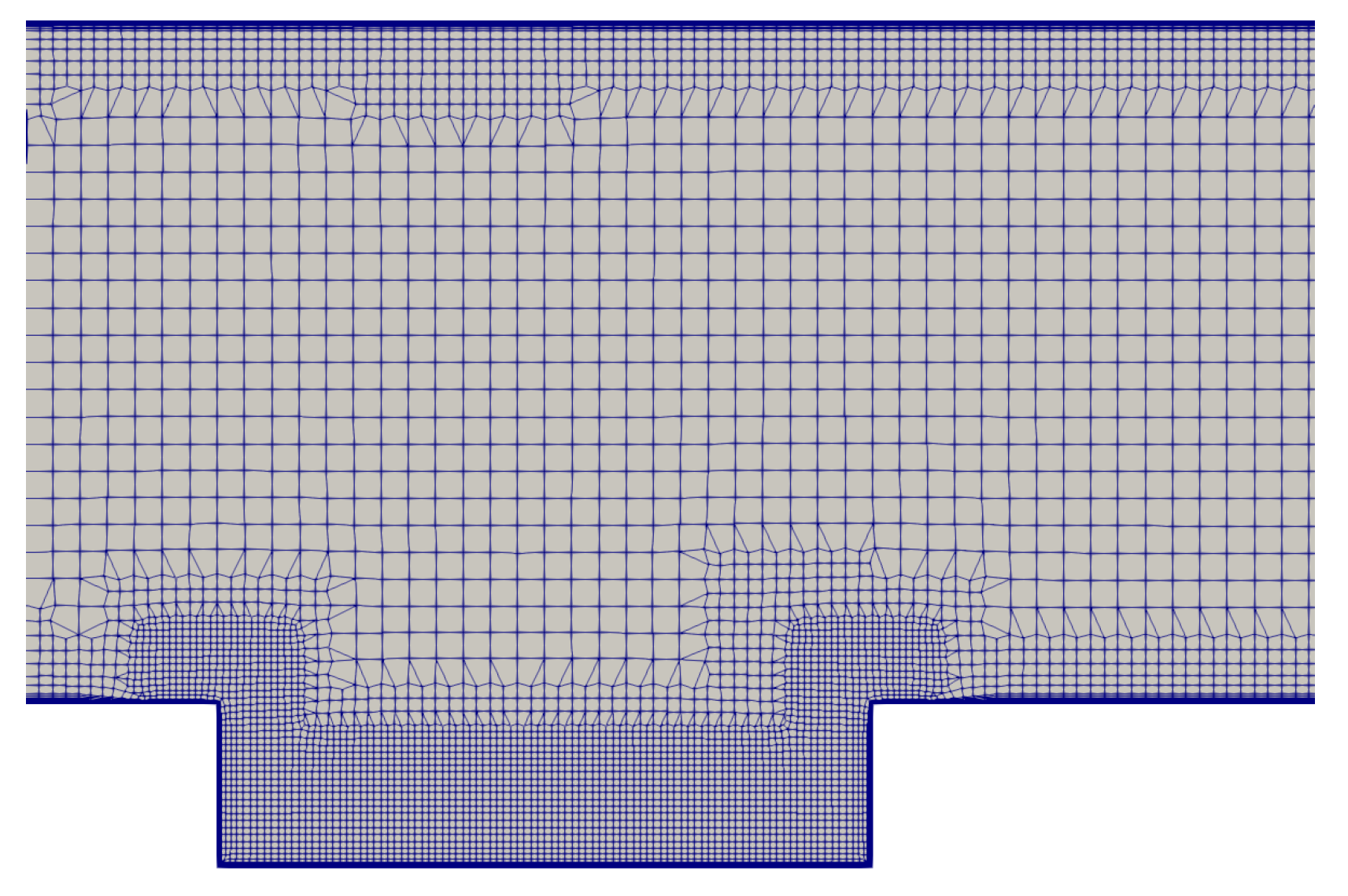
For the fluid domain study, meshes with different base element sizes and boundary layer thicknesses were compared. In all cases, the mesh was refined near walls and inside the cavity, and the refinement was equal to 0.5 of the base mesh size. The mesh looked similar in all cases; a part of the mesh is shown in Figure 3. The mesh consisted of 99% hexahedral elements, while the remaining elements were of polyhedral type, mainly made up of seven-face elements. Five meshes with the parameters described in Table 2 were compared and assessed. In all cases, structural mesh #3 (described in more detail later in this section) was used. For each of them, a solution was initiated with the SIMPLE algorithm and FSI simulations were carried out. Aluminum was used as the material of the cavity walls in every grid independence study simulation.
It should be emphasized here that the results obtained during the actual simulations may differ from those obtained in the analysis of mesh independence. This is due to the fact that after 0.1 s the flow may not have fully developed, as well as to the fact that in the proper simulations the calculated flow time was much longer and a different method of initiating the flow was used, that is, by solving the potential flow.
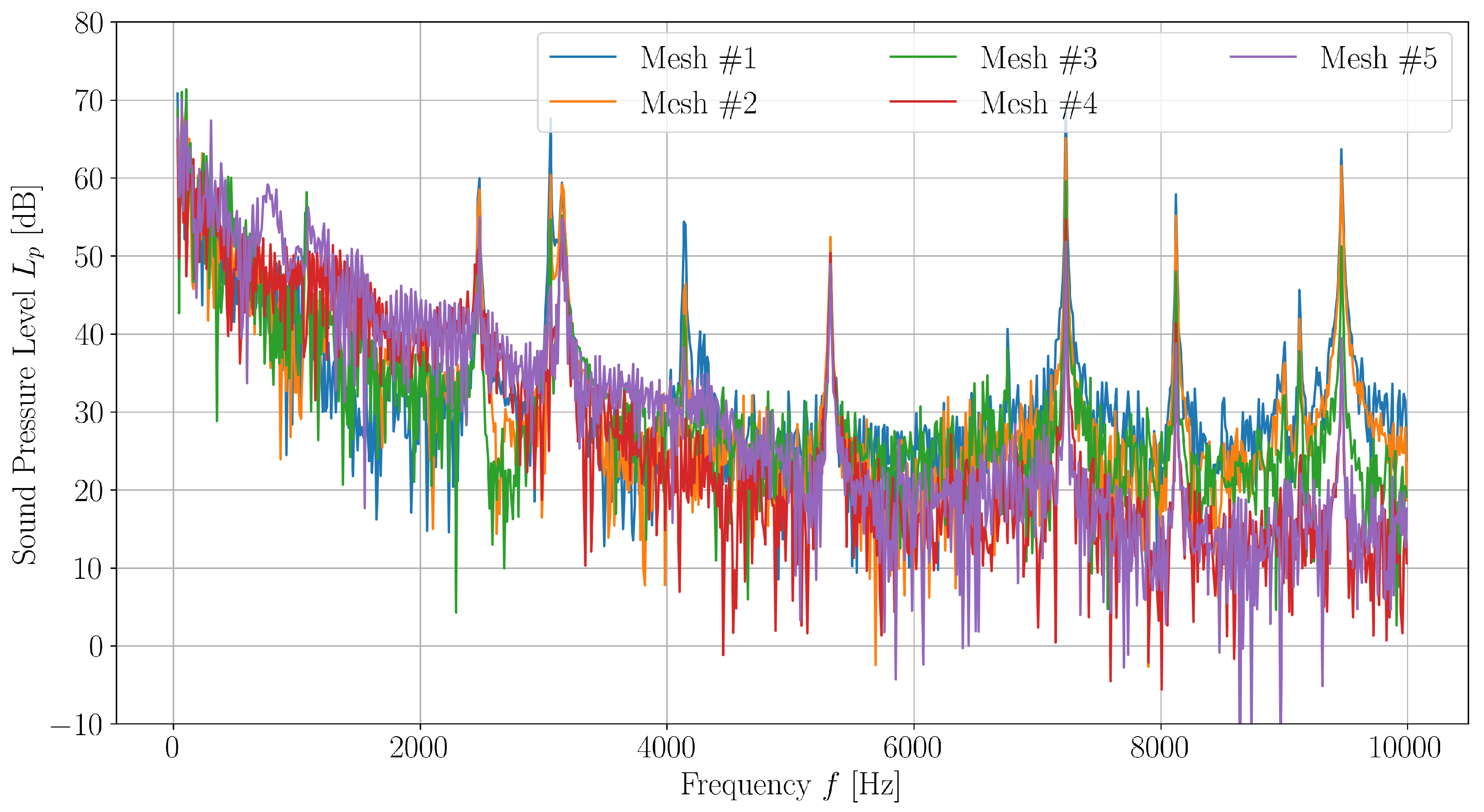
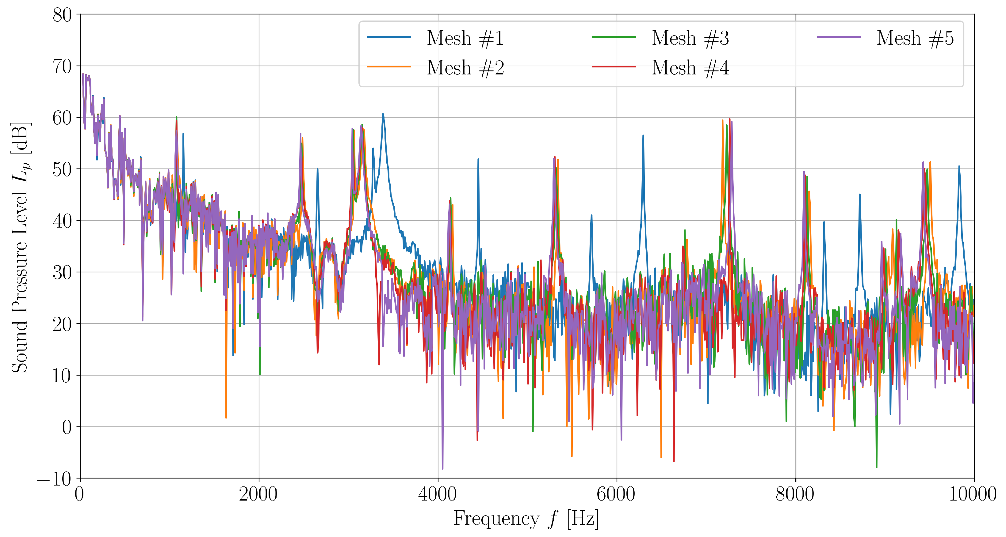
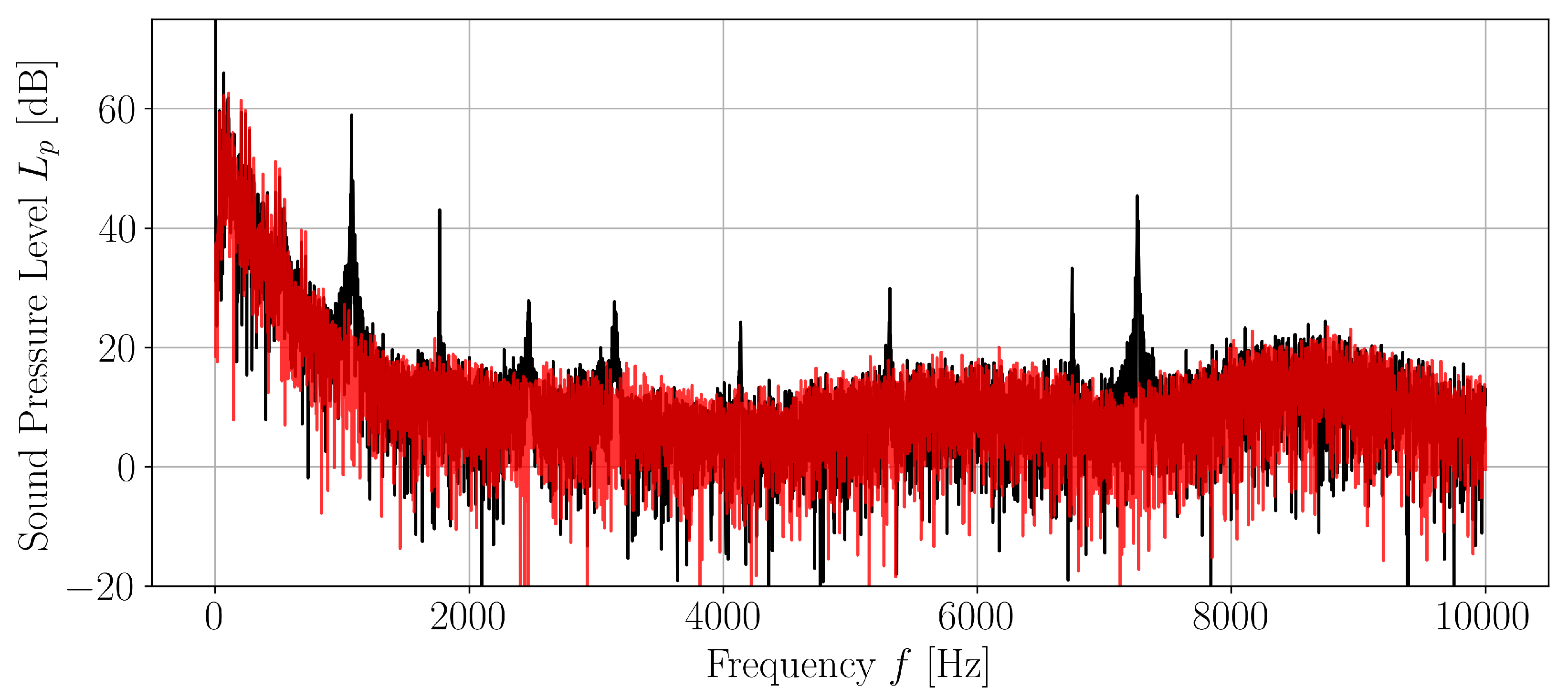
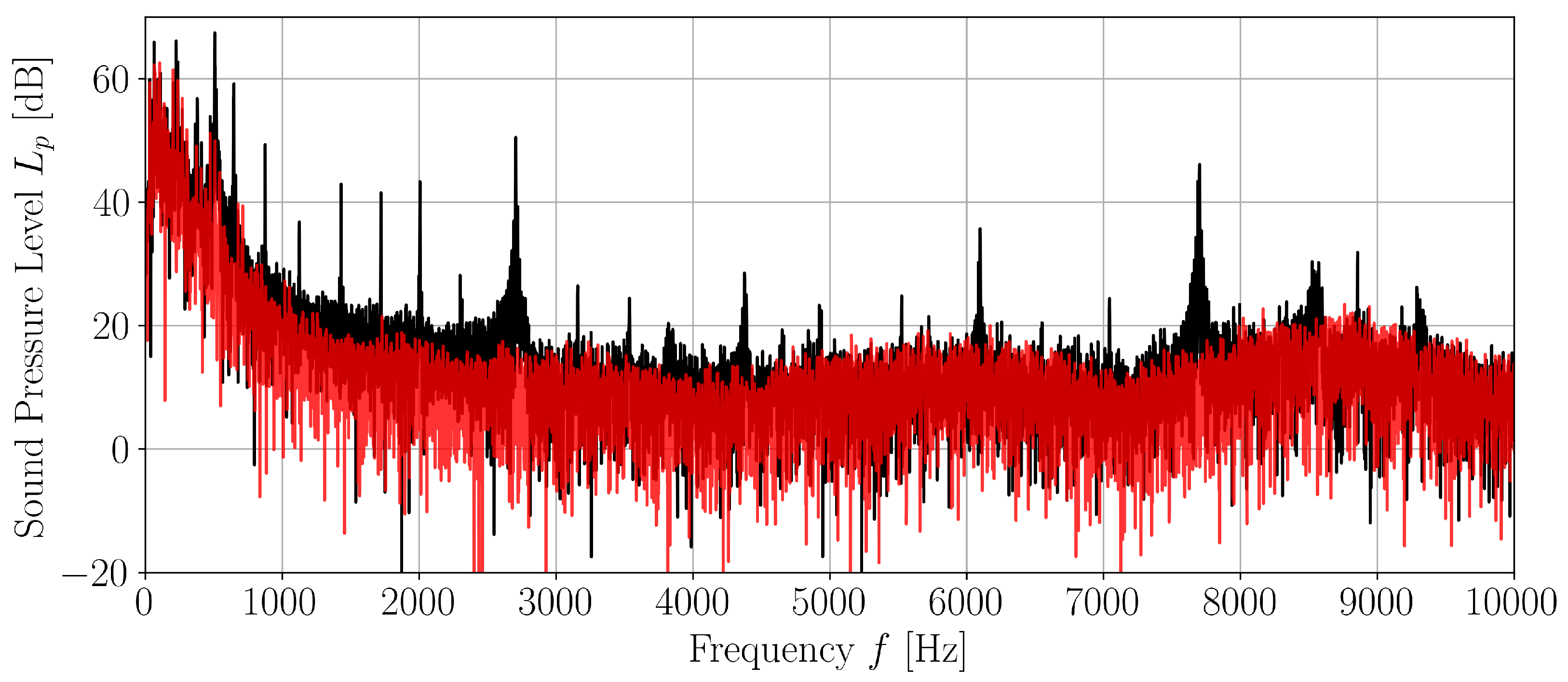
The results of sound pressure level evaluation at a receiver located 10 m from the middle of the cavity are shown in Figure 4. The spectra of the sound pressure level were similar in all cases, with characteristic peaks for the frequencies of 2.5, 3.1, 5.3, 7.3, 8.1, and 9 kHz. A decrease in the amplitude of the noise frequency components can be seen, along with an increase in the number of elements. Additionally, for grids #1 and #2, additional peaks appear at 4.1 ÷ 4.4 kHz.
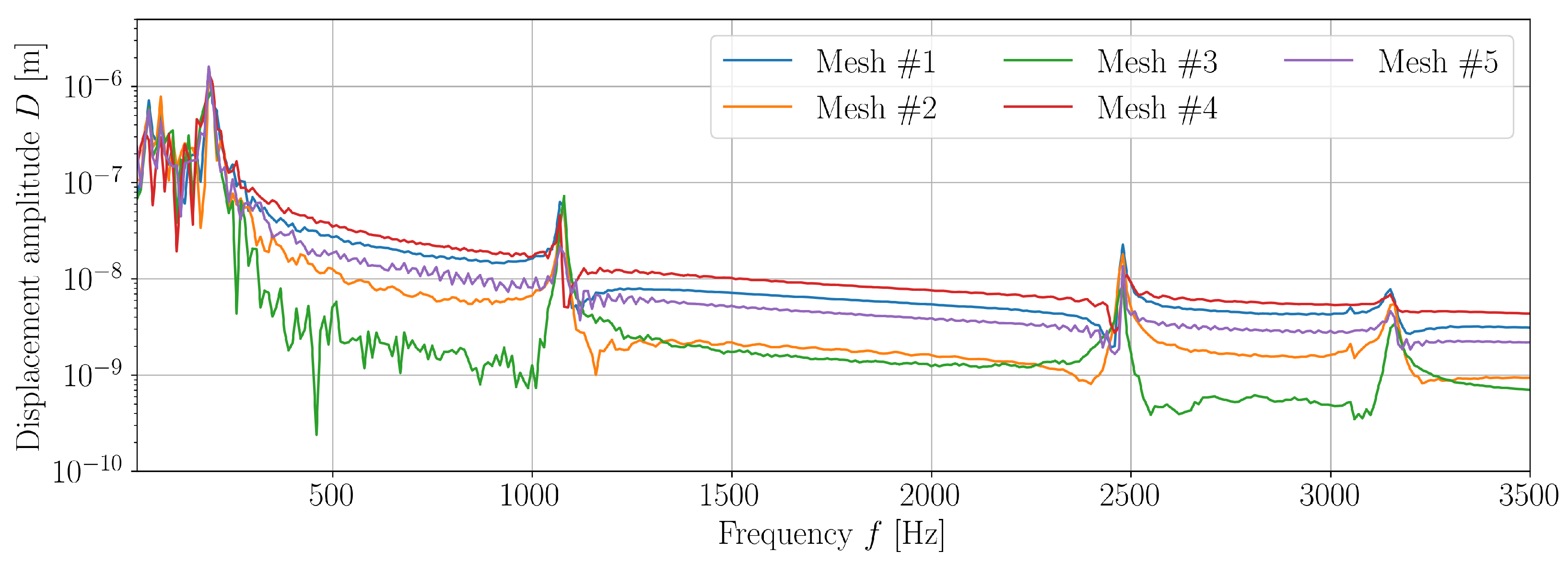
In addition, the spectra of the displacement of the cavity walls at probe S3 (Figure 2) were computed and are shown in the Figure 5. The results are again similar to each other; for the calculations on each mesh, there are peaks at the frequencies of 50 and 200 Hz. While there are additional frequency components above 1 kHz, they decrease as the number of mesh elements increases. Additional frequency components occurred below 100 Hz for meshes #1 and #2.
In Table 6, the values of the dimensionless wall distance y + for each wall are shown along with the time required to compute 0.1 s of the flow and the mean amplitude of vibrations at point S3. Meshes #3, #4, and #5 met the condition required by the turbulence model that this parameter should be less than one. The mean amplitude of vibrations were similar in all cases, with only the results for mesh #4 differing from the others.
Visible differences between the spectra for the different meshes may be due to the large size of the elements and the thickness of the boundary layer for flow meshes #1 and #2. The thickness of the boundary layer affects how the flow is resolved in it, while the size of the elements determines whether and which vortices and eddies are modeled or resolved directly. This translates into the obtained pressure distributions and forces acting on the walls. This, in turn, affects the values of displacements and deformations of the cavity walls and the acoustic pressure values obtained by means of acoustic analogies.
Based on the convergence analysis, it was decided to choose grid #3 for the remaining simulations. This choice was due to the relatively short calculation time while maintaining the required mesh parameters (parameter y + ) and lack of significant impact on the quality of the results from further mesh refinement.
The second independence study was focused on the structural mesh. Again, five different meshes were used in the simulations and the obtained results were compared with each other. All meshes for the structural simulations consisted of hexahedral elements, with the height and width of each element the same. The meshes were generated using the Frontal-Delaunay algorithm for quads. The parameter changed during the independence study was the base size of the element, which in turn was translated into the number of elements along the wall thickness.
All simulations were performed with fluid mesh #3, and aluminium was again used as the material of the cavity walls. The parameters of the used meshes are summarized in Table 3, along with time required to simulate 0.1 s of the flow and the mean amplitude of vibrations at probe S3.
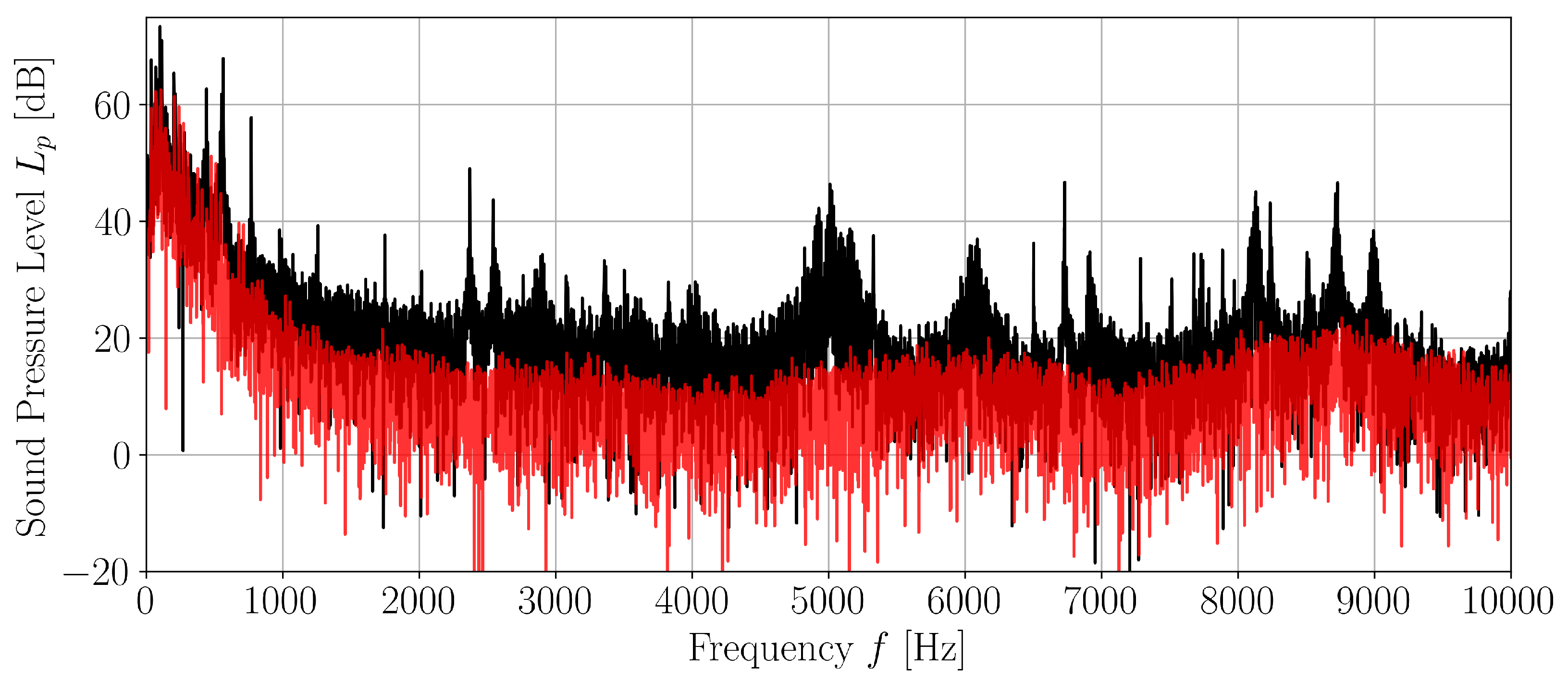
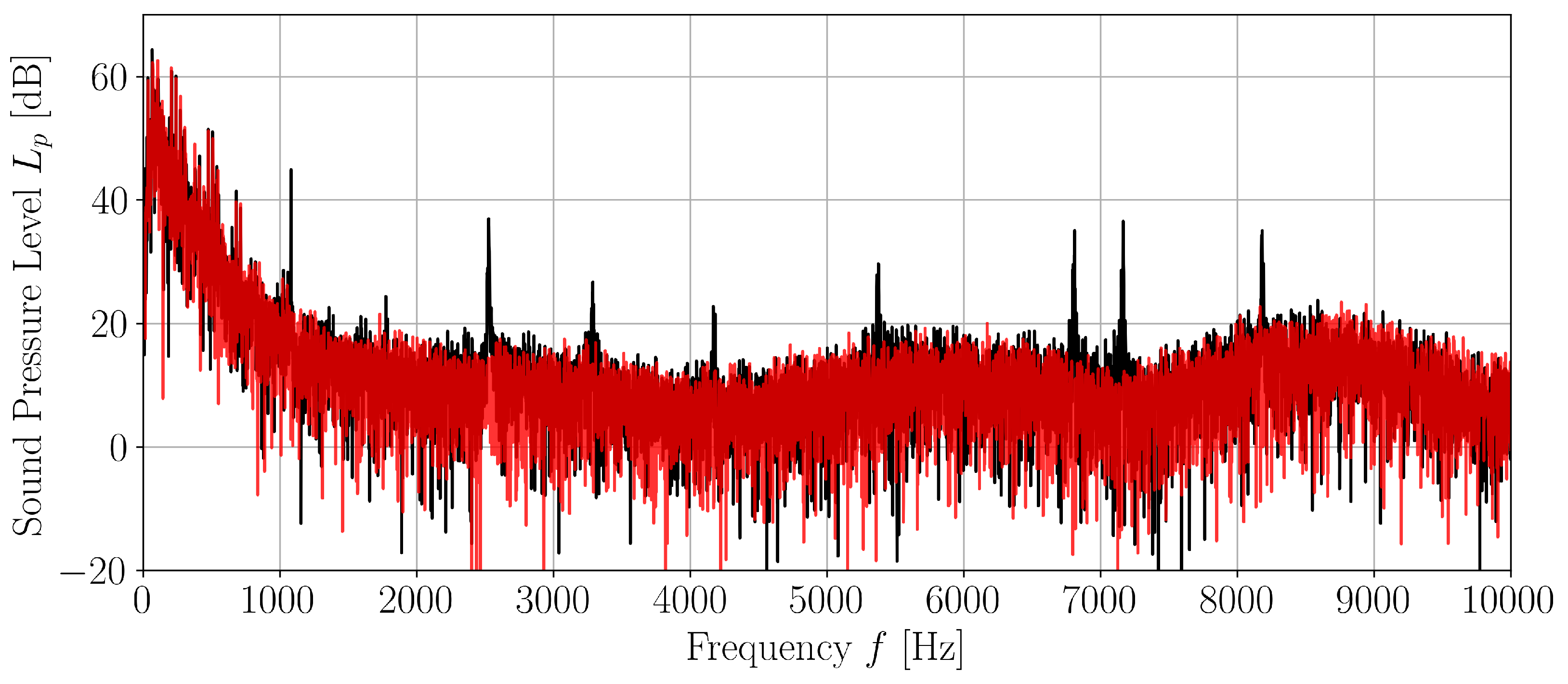
Figure 6 shows the sound pressure levels for at a receiver placed 10 m from the center of the cavity. For all meshes except #1, the results differed only slightly. The differences between the SPL spectra obtained using meshes #2–#5 increased with the frequency, although not significantly; for example, for the frequency of 7.3 kHz the maximum difference was 100 Hz, between mesh #2 and mesh #5. On the other hand, the results obtained for the first mesh differed significantly from the others, which may be due to an insufficient number of elements in the wall thickness. In addition, the sound pressure levels for mesh #2 differed from the results for the denser meshes, especially in the frequency range of 8.9–9.2 kHz.
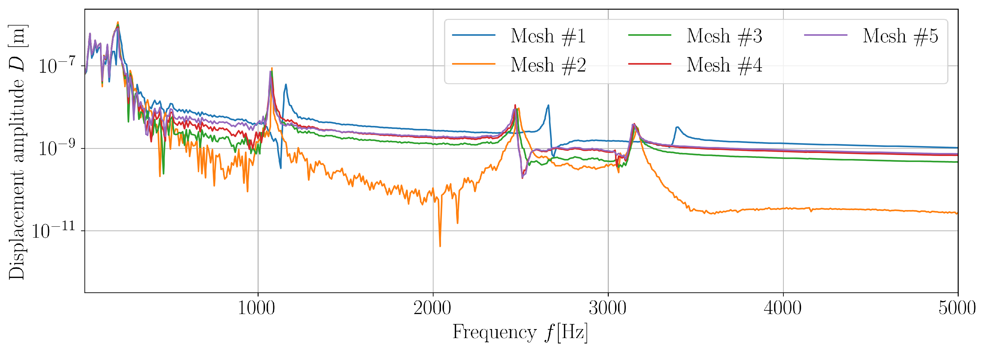
Similar conclusions can be drawn from the displacement amplitude spectra presented in Figure 7. It shows the spectrum of displacement of the cavity wall at point S3 for the simulation of each mesh. Again, the results for grid 1 are significantly different from the others, and there is a shift in frequency for the peaks at 1.1 and 2.5 kHz. Moreover, as the mesh becomes denser, the amplitudes for the peak at 200 Hz decrease.
Differences and shifts in the presented spectra, apart from the actual difference in the results, may be due to the relatively low time resolution of the results. It was not possible to simulate a longer flow time due to the fact that they were of relatively long duration anyway. However, even such a short time of calculations allowed us to draw conclusions about the convergence of the mesh. As can be seen from the presented data, further refinement of the mesh beyond mesh #4 does not improve the quality of the calculations. All simulations were carried out using grid #4. It was chosen for the reasons mentioned above, as well as for the fact that the computation time was only slightly longer than grid #3, and half that of grid #5. Moreover, a large number of elements in the thickness of the wall positively influenced the results.

4. Simulation Results

4.1. Flow Field

The results of the numerical simulations for the velocity and pressure fields are shown in Table 7. In all simulations, phenomena typical for flows over cavities can be seen, i.e., shear layer separation at the upstream edge, amplification of instabilities and vortices, impingement, vortex–downstream edge interactions (clipping and escape of vortices), and generation of pressure fluctuations [42]. The nature of the flows was relatively similar, and the introduction of flexible walls did not significantly affect the flow. However, in the case of the FSI model assuming walls made of polypropylene, deformation of the cavity resulted in the appearance of additional disturbances and eddies.
The flow pressure was sampled at points F1–F5 (Figure 1). The spectrum of pressure at point F3 is shown in Figure 8. In all cases, the highest peaks of pressure (largest vortices) appear at 34 Hz; however, their amplitudes differ. For the reference model and the model with steel as the wall material, it was 50 Pa, for the PVC and aluminium model it was 40 Pa, and for the polypropylene model it was 30 Pa. Smaller peaks appear at different frequencies depending on the material used.
As was mentioned in the introduction, Rossiter derived the equation linking the cavity dimensions, flow velocity, and frequencies of pressure fluctuations. The Rossiter model formula is provided by [6]:
f m = U L m γ 1 K + M
where U = 15 m / s is velocity, L = 0.12 m is the length of the cavity, m is the mode number, M = 0.44 is the Mach number, and γ ,   K are constants. Rossiter assumed γ = 0.25 and K = 0.57 , for a length to depth ratio equal to 4. In this work, the values of the constants γ = 0 and K = 0.28 were assumed, as the acoustic feedback can be considered as instantaneous [43,44].
The first ten computed Rossiter modes are shown in Table 8.
Rossiter stipulated that individual modes may or may not be excited. This is the case with the analyzed flows as well. The frequencies of 34 Hz and 69 Hz for which two highest peaks occured, as well as the frequency of 138 Hz, for which there is another increase in amplitude, are visible in Figure 8 and coincide with the first, second and fourth Rossiter modes.
The values of the unsteady pressure inside and in the vicinity of the cavity consist of two main components, periodic and random [6]. The analyzed cavities have a length to depth ratio of 4. Rossiter states that this ratio is a borderline case; below this ratio, periodic components predominate in the cavity, while above this ratio random components predominate. In the analyzed case, there are strong periodic components related to the Rossiter modes, while a random signal is present as well.
Thecalculated Rossiter modes are shown in Figure 8 as blue dashed vertical lines, and are compared with the flow pressure spectrum.

4.2. Cavity Wall Vibrations

In this section, the results of the simulations of vibrations of the structure are shown. The figures presented in Table 9 show the time evolution and frequency spectrum of displacement for each of the materials used in the FSI simulations. The amplitudes of vibration differ by several orders of magnitude, from 2.5 × 10 6 m for steel to 1.25 × 10 3 m for polypropylene; this displacement reaches 5% of total cavity depth, and can be seen in the distributions shown in the second row of Table 7. These differences result from the differences in the material parameters, more specifically, the changes in the Young’s modulus for each material.
In either case, the figures show significant peaks for specific frequencies. These dominant frequencies were compared with the results of the model analyses. The model analyses were performed using the same meshes, materials, and boundary conditions used in the coupled simulations. The results are shown and compared in Table 10. The vibration frequencies that coincide with the natural frequencies are marked in italics.
In addition, the graphs shown in Table 9 compare the frequencies of vibrations with the frequencies of the first six Rossiter modes, marked with vertical blue dashed lines. In most cases, the vibration peaks coincide with the frequencies of first three (or more) frequencies of the different modes. Moreover, Table 11 shows the shape of the first four modes for each material. The shapes shown there coincide with the flow snapshots, which show the displacement of the cavity walls. This is especially evident for polypropylene, shown in second row of Table 7. In the case of walls made of other materials, the deformations were too small to be visible.
In the case of aluminium, the highest frequency of vibrations at point S3 was equal to 190 Hz, the first mode of vibrations. The same happens for PVC and steel; for both materials, the highest peak frequency occurs at the frequency of the first mode of vibrations, 40.5 Hz and 192 Hz, respectively. For polyproplylene, the highest amplitude of vibration occurred at 35 Hz, both the first Rossiter mode and the first mode of vibrations. The high amplitude of vibrations of a structure made of this material may be due to the fact that these modes overlap, meaning that the vibrations are amplified.
In Figure 9 and Figure 10, the motion trajectories in the x-y plane of points S1–S5 are presented; the location of the points is shown in Figure 2. The time interval used to plot the trajectories was 0.8 to 0.9 s of the simulation time. Overall, it can be seen that the displacements of the bottom wall of the cavity are on average two orders of magnitude greater compared to the side walls. Moreover, the displacement of the upstream and downstream walls are similar both in order of magnitude and axisymmetrically, while the displacement amplitudes of the downstream wall are slightly larger. This is related to phenomena typical of flow over a cavity, namely, vortex shedding and its impingement on the downstream wall [45]. Depending on the material used, apart from the amplitudes of the displacements, their nature changes. The vibrations are regular for walls made of polypropylene, and the most irregular for walls made of PVC. This is especially visible on the trajectory plots of points S1 and S5. It should be noted that the trajectories for S2, S3, and S4 are not identical. This is related to various forms of natural vibrations and the fact that not every case has the highest amplitude in the first natural frequency.

4.3. Acoustic Pressure

Finally, we consider the aeroacoustic noise generated by the flow over the cavity and how flexible cavity walls affect it. In Figure 11, Figure 12, Figure 13 and Figure 14, the spectrum of sound pressure levels computed with the Ffowcs-Williams and Hawkings analogy (provided by Equation (23)) are shown. In each case, the receiver was defined as being positioned directly 5 m above the cavity. The sound pressure was sampled every 50 μs, which corresponds to a sampling frequency of 20 kHz. A rectangular window was used to find the FFT of the signal.
The sound pressure levels for all cases are shown in in Figure 11, Figure 12, Figure 13 and Figure 14. In each case, the results shown in black are compared with the sound pressure level computed for stiff walls, shown in red, which are repeated on each graph for clarity.
In all flow simulations involving the FSI model, significant differences between the spectra can be seen. In the low frequency range, up to 500 Hz, the spectra for all cases look similar and noise predominates. For the reference case with stiff walls, the sound pressue drops below 20 dB above 1000 Hz. A sound pressure level of 20 dB can be treated as lower than background noise for almost all rooms mentioned by the ASHRAE guide [46], and can therefore be omitted. These values may result from approximations and numerical errors. Compared to the reference case, for the frequencies below 500 Hz the sound pressure levels for the simulation with flexible walls have a similar character; however, peaks related to modal frequencies appear in the spectrum. Above 500 Hz, there is tonal noise that does not exist in the reference case. This is related to modal frequencies and natural vibrations.
As was mentioned in Section 4.2, Table 10 shows the natural frequencies of the cavity walls for all four cases. The bold text indicates the frequencies that coincide with the peaks of the spectra in Figure 11, Figure 12, Figure 13 and Figure 14. Regardless of the model adopted, in each case there was an increase in the amplitude close to the frequency of Rossiter modes, while, depending on the case, different modes were excited. In each of the cases, modes 1 and 2, 5, and 6 were excited, while modes 3 and 4 were excited only for the reference case and the cavity with polypropylene walls. This is due to the high sensitivity of this phenomenon to flow parameters, as well as to its high randomness.
The sound pressure levels above 1000 Hz as compared to the reference increase as the Young’s modulus of each material decreases. The Young’s modulus was the highest for steel. In the case of walls for which steel was adopted as a material, the spectra almost coincide, except for the few peaks mentioned above. As the Young’s modulus decreases, the average sound pressure level increases. The highest SPL was calculated for walls made of polypropylene; however, in this case, the result is not related only to the material used. For this material, the first Rossiter frequency coincides with the first natural frequency, which could further amplify the noise generated by the flow over the cavity.

5. Conclusions

In this work, the effects of elastic cavity walls and fluid–structure interaction on the noise generated by flow were investigated. Simulations were carried out for one geometric model selected on the basis of mesh independence analysis, one flow velocity, and four different sets of material parameters. In addition, flow analysis was carried out for the reference model, in which only unidirectional fluid–structure interaction was assumed and the walls were treated as rigid.
The main research findings and conclusions are as follows:
  • The simulations showed a significant effect of non-rigid walls and bidirectional fluid–structure interaction on flow noise.
  • In each of the analysed cases, the sound pressure level calculated using the FW-H acoustic analogy was higher than for the reference case with rigid walls, and the characteristics of the sound spectrum changed as well.
  • In the case of aeroacoustic analyses with flow through thin-walled channels, the fluid–structure interactions cannot be neglected.
  • In the case of the flow computations themselves, fluid–structure interactions are not as important; depending on the required accuracy of the results, they may be ignored.
  • Overlapping of natural and Rossiter frequencies can result in a significant increase in wall displacement amplitudes and sound pressure levels.
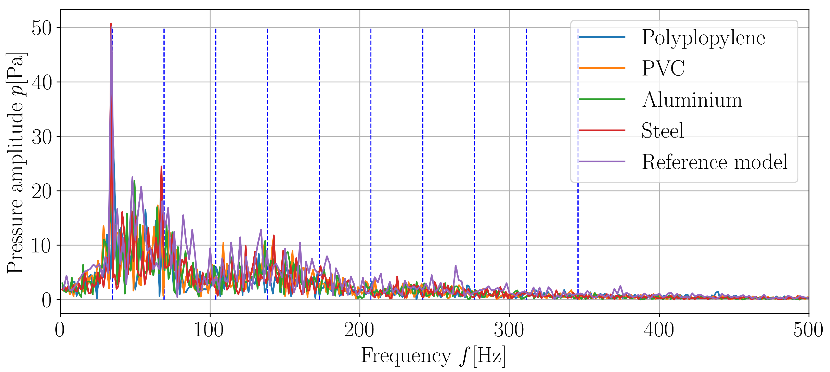
For the model with stiff walls, the SPL was similar throughout the band in the frequency range up to 1000 Hz, while above this range it fell below 20 dB. For the models with flexible walls, the sound pressure spectrum below 1000 Hz was similar to the reference case, while above this frequency there were additional components related to the movement of the cavity walls. Their frequencies partially coincided with the eigenfrequencies of the walls.
Overlapping between the natural and Rossiter frequencies occurred for one of the analysed materials (polypropylene). The overlapping of these frequencies at 35 Hz resulted in a significant increase in the wall displacement amplitude and sound pressure level. This should be borne in mind when designing ventilation systems. It is important to check that the Rossiter and natural frequencies do not coincide, as this can result in vibrations with high amplitudes.
The FW-H acoustic analogy was used to describe the flow-induced noise. Its limitations should be taken into account. This method does not account for the influence of the ventilation duct walls on the propagation of the acoustic wave along the duct, the propagation of the acoustic wave outside the duct, or vibroacoustic disturbances that could affect the obtained pressure level spectra.
The main purpose of this research was to verify whether the influence of the flow on the deformable walls of the cavity could affect the sound pressure levels, and this was achieved. In future research, it is necessary to investigate the influence of the remaining duct walls. In addition, it is necessary to investigate the influence of individual material parameters (as opposed to specific materials) on the flow and generated sound.
Here, it is worth mentioning several problems related to the modeling of fluid–structure interactions. Compared to calculations that do not take into account these interactions, both the computation time and the disk space needed to store the results are incomparably greater. Due to the limitations imposed by the PLGrid Infrastructure regarding the length of each task, it was necessary to perform a series of calculations in which the simulated time of each task was 0.1 s in order to compute 0.7 s of flow time. This was due to the imposed maximum duration of the simulations. The results were then combined for the purposes of this work. In the case of uncoupled CFD calculations for the same mesh and parameters, the time needed to simulate 0.1 s of the flow was 15 h. For simulations including FSI, it was over 150 h. Due to the size of the computational meshes, the simulations were performed in parallel on four and six computational nodes for the uncoupled and coupled models, respectively. Further increasing the number of nodes would not significantly affect computation time due to the time required for simulation data exchange between computational nodes. Moreover, for these simulations it was necessary to store information about both the flow field and the deformation field. Files with the results of these simulations were over 1.5 TB in size. Because of this, it would be impossible to conduct such analyses without the use of PLGrid Infrastructure and its computing resources.

Author Contributions

Conceptualization, P.Ł., I.C. and A.G.; methodology, P.Ł. and I.C.; software, P.Ł.; validation, P.Ł. and I.C.; formal analysis, P.Ł.; investigation, P.Ł.; resources, P.Ł.; data curation, P.Ł. and I.C.; writing—original draft preparation, P.Ł.; writing—review and editing, I.C. and A.G.; visualization, P.Ł. and I.C.; supervision, I.C. and A.G.; project administration, I.C.; funding acquisition, A.G. All authors have read and agreed to the published version of the manuscript.

Funding

This research was supported by national subvention no. 16.16.130.942.

Acknowledgments

This research was supported in part by PLGrid Infrastructure.

Conflicts of Interest

The authors declare no conflict of interest.

Nomenclature

v i = v i ¯ + v i ith component of velocity [m/s]
p = p ¯ + p pressure [Pa]
ρ density [kg/m 3 ]
τ i j ¯ laminar viscous stress tensor [N/m 2 ]
τ i j R = ρ v i v j ¯ Reynolds stress tensor [N/m 2 ]
ψ ¯ mean/filtered variable [-]
ψ fluctuating/sub-filter variable [-]
μ t eddy viscosity [m 2 /s]
kturbulent kinetic energy [m 2 /s 2 ]
ω specific dissipation rate [1/s]
β * , σ k σ ω , γ , a 1 constants of the k ω SST turbulence model
F 1 , F 2 additional functions of the k ω SST turbulence model
T i j S = u ¯ i u ¯ j u i u j ¯ subgrid-scale (SGS) stress tensor [N/m 2 ]
U ¨ = A global acceleration vector [m/s 2 ]
Uglobal displacement vector [m]
Mglobal mass matrix [kg]
Kglobal stiffness matrix [N/m]
Fglobal force vector [N]
Σ K L M N free energy function [kg m 2 /s 2 ]
θ absolute temperature [K]
ρ 0 mass density [kg/m 3 ]
f k force per unit mass [N/kg]
β K L thermal stress tensor per unit temperature [N/m 2 K]
γ K L residual stress tensor [N/m 2 ]
φ shape function [-]
ξ i , η i , ζ i local coordinates of the ith point
ρ (acoustic) density fluctuations [kg/m 3 ]
H s Heaviside step function [-]
T i j Lighthill stress tensor [N/m 2 ]
c speed of sound [m/s]
V i velocity of surface in i direction [m/s]
fscalar function defining the surface [-]
δ Dirac delta function [-]

Abbreviations

The following abbreviations are used in this manuscript:
ASHRAEAmerican Society of Heating, Refrigerating, and Air-Conditioning Engineers
CAAComputational Aeroacoustics
CFDComputational Fluid Dynamics
DESDetached Eddy Simulation
FFTFast Fourier Transform
FSIFluid–Structure Interaction
FWHFfowcs-Williams and Hawkings (acoustic analogy)
LESLarge Eddy Simulation
PISOPressure-Implicit with Splitting of Operators
PVCPolyvinyl Chloride
RANSReynolds-Averaged Navier–Stokes
SGSSub-Grid Scale
SIMPLESemi-Implicit Method for Pressure-Linked Equations
SPLSound Pressure Level
SSTShear Stress Transport

References

  1. Crook, S.; Kelso, R.; Drobik, J. Aeroacoustics of Aircraft Cavities. In Proceedings of the 16th Australian Fluid Mechanics Conference, Gold Coast, Australia, 3–7 December 2007. [Google Scholar]
  2. Wang, Z.K.; Djambazov, G.; Lai, C.H.; Pericleous, K. Numerical simulation of flow-induced cavity noise in self-sustained oscillations. Comput. Vis. Sci. 2007, 10, 123–134. [Google Scholar] [CrossRef]
  3. Kim, H.; Hu, Z.; Thompson, D. Effect of cavity flow control on high-speed train pantograph and roof aerodynamic noise. Railw. Eng. Sci. 2020, 28, 54–74. [Google Scholar] [CrossRef] [Green Version]
  4. Radavich, P.M.; Selamet, A.; Novak, J.M. A computational approach for flow–acoustic coupling in closed side branches. J. Acoust. Soc. Am. 2001, 109, 1343–1353. [Google Scholar] [CrossRef] [PubMed] [Green Version]
  5. Lafon, P.; Caillaud, S.; Devos, J.; Lambert, C. Aeroacoustical coupling in a ducted shallow cavity and fluid/structure effects on a steam line. J. Fluids Struct. 2003, 18, 695–713. [Google Scholar] [CrossRef]
  6. Rossiter, J.E. Wind Tunnel Experiments on the Flow over Rectangular Cavities at Subsonic and Transonic Speeds. 1964. Available online: https://reports.aerade.cranfield.ac.uk/handle/1826.2/4020 (accessed on 1 October 2022).
  7. Rockwell, D.; Naudascher, E. Review—Self-Sustaining Oscillations of Flow Past Cavities. J. Fluids Eng. 1978, 100, 152–165. [Google Scholar] [CrossRef]
  8. Yokoyama, H.; Hibino, K.; Nishikawara, M.; Yanada, H. Oscillations of a flexible beam in cavity flow with tonal sound. In Proceedings of the 6th International Conference of Global Network for Innovative Technology (IGNITE), Penang, Malaysia, 2–3 December 2019. [Google Scholar]
  9. Thangamani, V.; Kok, F.N. Energy harvesting from cavity flow oscillations. J. Intell. Mater. Syst. Struct. 2022, 33, 400–418. [Google Scholar] [CrossRef]
  10. Khanafer, K. Comparison of flow and heat transfer characteristics in a lid-driven cavity between flexible and modified geometry of a heated bottom wall. Int. J. Heat Mass Transf. 2014, 78, 1032–1041. [Google Scholar] [CrossRef]
  11. Alsabery, A.; Selimefendigil, F.; Hashim, I.; Chamkha, A.; Ghalambaz, M. Fluid-structure interaction analysis of entropy generation and mixed convection inside a cavity with flexible right wall and heated rotating cylinder. Int. J. Heat Mass Transf. 2019, 140, 331–345. [Google Scholar] [CrossRef]
  12. Sun, X.; Li, W.; Ye, Z. Flow-induced Vibration of Flexible Bottom Wall in a Lid-driven Cavity. J. Vib. Test. Syst. Dyn. 2017, 1. [Google Scholar] [CrossRef]
  13. Sabbar, W.A.; Ismael, M.A.; Almudhaffar, M. Fluid-structure interaction of mixed convection in a cavity-channel assembly of flexible wall. Int. J. Mech. Sci. 2018, 149, 73–83. [Google Scholar] [CrossRef]
  14. Strelets, M. Detached eddy simulation of massively separated flows. In Proceedings of the 39th Aerospace Sciences Meeting and Exhibit, Reno, NV, USA, 8–11 January 2001. [Google Scholar]
  15. Menter, F. Zonal Two Equation k-ω Turbulence Models For Aerodynamic Flows. In Proceedings of the 23rd Fluid Dynamics, Plasmadynamics, and Lasers Conference, Orlando, FL, USA, 6–9 July 1993. [Google Scholar]
  16. Wagner, C.; Huttl, T.; Sagaut, P. Large-Eddy Simulaton for Acoustics; Cambridge University Press: Cambridge, UK, 2007. [Google Scholar]
  17. Hu, J.; Ning, X.; Zhao, W.; Li, F.; Ma, J.; Zhang, W.; Sun, S.; Zou, M.; Lin, C. Numerical simulation of the cavitating noise of contra-rotating propellers based on detached eddy simulation and the Ffowcs Williams–Hawkings acoustics equation. Phys. Fluids 2021, 33, 115117. [Google Scholar] [CrossRef]
  18. Sharma, S.; Geyer, T.F.; Giesler, J. Effect of geometric parameters on the noise generated by rod-airfoil configuration. Appl. Acoust. 2021, 177, 107908. [Google Scholar] [CrossRef]
  19. Liu, K.; Zhou, S.; Li, X.; Shu, X.; Guo, L.; Li, J.; Zhang, X. Flow-induced noise simulation using detached eddy simulation and the finite element acoustic analogy method. Adv. Mech. Eng. 2016, 8. [Google Scholar] [CrossRef] [Green Version]
  20. Bungartz, H.J.; Lindner, F.; Gatzhammer, B.; Mehl, M.; Scheufele, K.; Shukaev, A.; Uekermann, B. preCICE—A fully parallel library for multi-physics surface coupling. Comput. Fluids 2016, 141, 250–258. [Google Scholar] [CrossRef]
  21. Lighthill, M.J. On Sound Generated Aerodynamically. I. General Theory. Proc. R. Soc. Lond. Ser. A Math. Phys. Sci. 1952, 211, 564–587. [Google Scholar]
  22. Williams, J.E.F.; Hawkings, D.L. Sound generation by turbulence and surfaces in arbitrary motion. Philos. Trans. R. Soc. Lond. Ser. A Math. Phys. Sci. 1969, 264, 321–342. [Google Scholar]
  23. Rama krishna, V.; Sanaka, S.P.; Pardhasaradhi, N.; Raghava Rao, B. Hydro-elastic computational analysis of a marine propeller using two-way fluid structure interaction. J. Ocean Eng. Sci. 2021. [Google Scholar] [CrossRef]
  24. Ma, R.; Liu, Z.; Zhang, G.; Doolan, C.J.; Moreau, D.J. Acoustic analysis of a forced-oscillating cylinder in flow using a hybrid method. Aerosp. Sci. Technol. 2020, 106. [Google Scholar] [CrossRef]
  25. Turek, S.; Hron, J. Proposal for Numerical Benchmarking of Fluid–Structure Interaction Between an Elastic Object and Laminar Incompressible Flow. Fluid-Struct. Interact. Model. Simul. Optim. 2007, 53, 371–385. [Google Scholar]
  26. Chourdakis, G.; Davis, K.; Rodenberg, B.; Schulte, M.; Simonis, F.; Uekermann, B.; Abrams, G.; Bungartz, H.J.; Yau, L.; Desai, I.; et al. preCICE v2: A Sustainable and User-Friendly Coupling Library. Open Res. Eur. 2022, 2, 51. [Google Scholar] [CrossRef]
  27. Lojek, P.; Czajka, I.; Golas, A.; Suder-Debska, K. Infuence of the Elastic Cavity Walls on Cavity Flow Noise. Vib. Phys. Syst. 2021, 1. [Google Scholar]
  28. III, L.N.C.; Garg, S.; Washburn, A.E. Piezoelectric actuators for fluid-flow control. In Proceedings of the Smart Structures and Materials 1997: Industrial and Commercial Applications of Smart Structures Technologies; Sater, J.M., Ed.; International Society for Optics and Photonics: San Diego, CA, USA, 1997; Volume 3044, pp. 147–157. [Google Scholar]
  29. Chatellier, L.; Laumonier, J.; Gervais, Y. Active control of the aeroacoustics of cavity flows from the downstream edge. C. R. Méc. 2006, 334, 259–265. [Google Scholar] [CrossRef]
  30. Blazek, J. Computational Fluid Dynamics. Principles and Applications; Elsevier Ltd.: Amsterdam, The Netherlands, 2015. [Google Scholar]
  31. Weller, H.G.; Tabor, G.R.; Jasak, H.; Fureby, C. A tensorial approach to computational continuum mechanics using object-oriented techniques. Comput. Phys. 1998, 12, 620–631. [Google Scholar] [CrossRef]
  32. Holzmann, T. Mathematics, Numerics, Derivations and OpenFOAM(R). 2019. Available online: https://holzmann-cfd.com/community/publications/mathematics-numerics-derivations-and-openfoam (accessed on 1 October 2022).
  33. Patankar, S.; Spalding, D. A calculation procedure for heat, mass and momentum transfer in three-dimensional parabolic flows. Int. J. Heat Mass Transf. 1972, 15, 1787–1806. [Google Scholar] [CrossRef]
  34. Issa, R. Solution of the implicitly discretised fluid flow equations by operator-splitting. J. Comput. Phys. 1986, 62, 40–65. [Google Scholar] [CrossRef]
  35. Dhondt, G. The Finite Element Method for Three-Dimensional Thermomechanical Applications; John Wiley & Sons Ltd.: Hoboken, NJ, USA, 2004. [Google Scholar]
  36. Lapidus, L.; Pinder, G. Numerical Solution of Partial Differential Equations in Science and Engineerig; John Wiley & Sons Ltd.: Hoboken, NJ, USA, 1999. [Google Scholar]
  37. Glegg, S.; Devenport, W. Aeroacoustics of Low Mach Number Flows—Fundamentals, Analysis and Measurement; Academic Press: Cambridge, MA, USA, 2017. [Google Scholar]
  38. Brentner, K.S.; Farassat, F. Modeling aerodynamically generated sound of helicopter rotors. Prog. Aerosp. Sci. 2003, 39, 83–120. [Google Scholar] [CrossRef] [Green Version]
  39. Epikhin, A.; Evdokimov, I.; Kraposhin, M.; Kalugin, M.; Strijhak, S. Development of a Dynamic Library for Computational Aeroacoustics Applications Using the OpenFOAM Open Source Package. Procedia Comput. Sci. 2015, 66, 150–157. [Google Scholar] [CrossRef] [Green Version]
  40. Komerath, N.; Ahuja, K.; Chambers, F. Prediction and measurement of flows over cavities—A survey. In Proceedings of the 25th AIAA Aerospace Sciences Meeting, Reno, NV, USA, 24–26 March 1987. [Google Scholar]
  41. ASHRAE Handbook—HVAC Systems and Equipment; ASHRAE: Atlanta, GA, USA, 2016.
  42. Gloerfelt, X. Cavity Noise. 2007. Available online: https://www.researchgate.net/publication/292356579_Cavity_noise (accessed on 1 October 2022).
  43. Ma, R.; Slaboch, P.; Morris, S. Fluid mechanics of the flow-excited Helmholtz resonator. J. Fluid Mech. 2009, 623. [Google Scholar] [CrossRef]
  44. Verdugo, F.; Guitton, A.; Camussi, R. Experimental investigation of a cylindrical cavity in a low Mach number flow. J. Fluids Struct. 2012, 28. [Google Scholar] [CrossRef]
  45. Knisely, C.; Rockwell, D. Self-sustained low-frequency components in an impinging shear layer. J. Fluid Mech. 1982, 116. [Google Scholar] [CrossRef]
  46. ASHRAE Handbook—HVAC Applications; ASHRAE: Atlanta, GA, USA, 2019.
Figure 1. Analyzed model of cavity with probe locations.
Energies 15 08017 g001
Figure 2. Boundaries of the finite element model with probe locations.
Energies 15 08017 g002
Figure 3. Computational mesh for fluid simulations (case #2).
Energies 15 08017 g003
Figure 4. Sound pressure level at observer 10 m from center of the cavity for finite volume mesh independence study.
Energies 15 08017 g004
Figure 5. Spectrum of displacement along y axis at probe S3 for finite volume mesh independence study.
Energies 15 08017 g005
Figure 6. Sound pressure level at observer 10 m from center of the cavity for finite element mesh independence study.
Energies 15 08017 g006
Figure 7. Spectrum of displacement along the y axis at probe S3 for finite element mesh independence study.
Energies 15 08017 g007
Figure 8. Spectrum of flow pressure at point F3 (Figure 1) (Energies 15 08017 i039 Rossiter modes).
Energies 15 08017 g008
Figure 9. Displacement d y - d x trajectories of points S1 and S5 for each material (in meters).
Energies 15 08017 g009
Figure 10. Displacement d y - d x trajectories of points S2, S3 and S4 for each material (in meters).
Energies 15 08017 g010
Figure 11. Sound pressure level of cavity noise with flexible aluminium walls (Energies 15 08017 i037) and stiff walls (Energies 15 08017 i038).
Energies 15 08017 g011
Figure 12. Sound pressure level of cavity noise with flexible polypropylene walls (Energies 15 08017 i037) and stiff walls (Energies 15 08017 i038).
Energies 15 08017 g012
Figure 13. Sound pressure level of cavity noise with flexible PVC walls (Energies 15 08017 i037) and stiff walls (Energies 15 08017 i038).
Energies 15 08017 g013
Figure 14. Sound pressure level of cavity noise with flexible steel walls (Energies 15 08017 i037) and stiff walls (Energies 15 08017 i038).
Energies 15 08017 g014
Table 1. Dimensions of the model (in meters).
hDL l 1 l 2
0.1250.030.120.10.5
Table 2. Mesh parameters for finite volume grid independence study.
MeshElement Size [mm]Boundary Layer Thickness [mm]Number of ElementsAspect RatioAverage Non-Orthogonality
#15114,31427.12.14
#23132,75440.81.52
#31.50.7599,89638.20.89
#410.5202,23027.10.78
#50.750.25337,50840.80.57
Table 3. Mesh parameters for finite element grid independence study with simulation time and mean amplitude of vibrations.
Base Element Size [m]Elements Along WallNumber of ElementsSimulation Time [h]Mean Amplitude of Vibrations [m]
Mesh #10.00032120816 2.88 × 10 6
Mesh #20.0001610,87234 3.01 × 10 6
Mesh #30.00008818,18750 3.03 × 10 6
Mesh #40.000061030,20078 3.04 × 10 6
Mesh #50.000041567,975156 3.05 × 10 6
Table 4. Fluid simulation boundary conditions.
Pressure p / ρ   [ m 2 / s 2 ] Velocity v
[m/s]
Turbulence Kinetic Energy k  [ m 2 / s 2 ] Specific Dissipation Rate ω [1/s]Turbulent Viscosity ν t   [ m 2 / s ]
Inlet p x n = 0 u x = 15 , u y , z = 0 k = 3.375 ω = 2500 calculated
Outlet p = 0 u i x n = 0 k x n = 0 ω x n = 0 calculated
Walls p x n = 0 u i = 0 k = 0 ω = 8 × 10 6 ν t = 0
Table 5. Properties of materials used for structural modeling.
MaterialYoung’s Modulus E [Pa]Poisson’s Ratio ν [-]Density ρ [kg/m 3 ]
Polypropylene 900 × 10 6 0.421100
Polyvinyl chloride (PVC) 1.5 × 10 9 0.421400
Aluminium 70 × 10 9 0.332700
Structural steel 210 × 10 9 0.297800
Table 6. Parameter y + , time of simulation, and amplitude of vibrations at point S3 for different meshes.
y + at Top Wall y + at Bottom Wall y + at Cavity WallsSimulation Time [h]Mean Amplitude of Vibrations [m]
Mesh #12.72.10.8635 3.31 × 10 6
Mesh #21.451.20.648 2.94 × 10 6
Mesh #30.630.490.2750 3.19 × 10 6
Mesh #40.430.420.1671 1.99 × 10 6
Mesh #50.290.260.1484 2.66 × 10 6
Table 7. Contours of velocity and pressure for reference models and FSI models with different materials at t = 1 s.
Velocity Magnitude [m/s]
Energies 15 08017 i001
Pressure [Pa]
Energies 15 08017 i002
Stiff wallsEnergies 15 08017 i003Energies 15 08017 i004
Polyprop.Energies 15 08017 i005Energies 15 08017 i006
PVCEnergies 15 08017 i007Energies 15 08017 i008
AluminiumEnergies 15 08017 i009Energies 15 08017 i010
SteelEnergies 15 08017 i011Energies 15 08017 i012
Table 8. Cavity Rossiter modes computed with Equation (24) for γ = 0.25 and K = 0.57 .
Mode Number12345678910
Frequency f R [Hz]34.5769.14103.71138.29172.86207.43242.01276.58311.15345.73
Table 9. Time evolution and frequency spectra of displacement at point S3 for different materials (Energies 15 08017 i039 Rossiter Modes).
PolypropyleneDisplacement y [m]Energies 15 08017 i013Energies 15 08017 i014
PVCDisplacement y [m]Energies 15 08017 i015Energies 15 08017 i016
AluminiumDisplacement y [m]Energies 15 08017 i017Energies 15 08017 i018
SteelDisplacement y [m]Energies 15 08017 i019Energies 15 08017 i020
Time t [s]Frequency f [Hz]
Table 10. Computed natural frequencies for each material (in Hz) (italics—frequencies that coincide with cavity wall vibration spectrum frequency peaks (Section 4.2), bold—frequencies that coincide with noise spectrum frequency peaks (Section 4.3)).
Mode NumberPolypropylenePVCAluminiumSteel
135.440.5190.8192.4
241.947.9231.3234.8
344.851.3241.7243.6
4103.6118.6558.7563.2
5109.1124.9596.4603.7
6198.1226.71068.51077.0
7208.7238.81134.51146.5
8327.1374.31764.11778.2
9338.3387.11834.01851.9
10467.0534.52518.32538.4
11478.0547.02587.02610.8
12560.5641.43030.23057.2
13568.7650.83065.63089.9
14616.1705.03321.43347.9
15624.7714.93374.73404.0
16768.6879.54144.34177.6
17773.3884.94179.64216.3
18989.91132.85339.05382.1
191001.21145.75409.45456.2
201252.41433.16754.76809.3
Table 11. Computed shapes of first four modes for different materials.
Mode 1Mode 2Mode 3Mode 4
Polyprop.Energies 15 08017 i021Energies 15 08017 i022Energies 15 08017 i023Energies 15 08017 i024
PVCEnergies 15 08017 i025Energies 15 08017 i026Energies 15 08017 i027Energies 15 08017 i028
AluminiumEnergies 15 08017 i029Energies 15 08017 i030Energies 15 08017 i031Energies 15 08017 i032
SteelEnergies 15 08017 i033Energies 15 08017 i034Energies 15 08017 i035Energies 15 08017 i036
Publisher’s Note: MDPI stays neutral with regard to jurisdictional claims in published maps and institutional affiliations.

