Identification of the Dynamic Properties of the Coal Flotation Process as a Control Object with the Use of the Kalman Filter

Abstract

For various sorts of hard coal, enrichment by flotation is used for feed consisting of grains smaller than 0.5 mm. Regarding process automation, coal flotation is a multidimensional, dynamic nonlinear object of control, for which the main control signal is the flow rate of the flotation agent. Typically, in Polish coal-processing facilities the monitoring and control systems of the flotation process can only measure the parameter of the waste quality (content of ash in flotation tailings). This naturally becomes an output signal, enabling an indirect assessment of the ongoing process. Therefore, knowledge of the dynamic properties of the flotation process, analysed as an object with one control input (the flow rate of the flotation agent) and with one output for measuring (content of ash in flotation tailings) may be material in designing automatic control systems for this operation. It is important to use an appropriate identification method when developing a model of the dynamics of the flotation process, especially if the model parameters are to be determined on an ongoing basis. This article discusses the research method and presents the results of applying the method of identifying the dynamic properties of the coal flotation process with the use of the Kalman filter. We carried out a comparative analysis of the results obtained by this method based on the Kalman algorithm and the method of least squares, taken as the reference method. The presented parameters of the dynamic models were calculated based on actual data obtained from industrial tests conducted at the coal-processing plant at one of the Polish mines. It was demonstrated that, for control purposes, the Kalman algorithm can be successfully applied in identification of the coal flotation process. This is due to the fact that it gives satisfactory results in relation to the adopted reference method despite the fact that it is a recursive algorithm.

1. Introduction

Coal flotation is the most effective technique used to improve the nature of fine particles by reducing contaminants and has been the subject of many studies [1,2,3,4,5,6]. In Polish coal-processing facilities, the flotation process is a side enrichment process as the feed consists of grains smaller than 1 mm. In industrial practice there are usually measured quantitative parameters of the feed, such as flow rate (qn) and concentration of solids in the feed (kcs). Electromagnetic flow meters are used to measure the flow rate of the feed [7]. Concentration of solid particles is usually measured using a radiometric density meter and less commonly a piezometric meter [7,8,9,10,11]. However, the ash content in the feed (an) is not available for measurement. Of the output signals, which refer to quantitative and qualitative parameters of flotation products, the only one available for measurement is ash content in flotation tailings (ao). This quantity is measured using the MPOF optical ash meter [7,10,12]. Quantitative and qualitative parameters of the concentrate (commercial product) are determined on the basis of periodic sampling, the values of which are determined by laboratory methods. Thus, due to the limited measurement information available on an ongoing basis, the content of ash in flotation tailings becomes a parameter that enables indirect assessment of the quality of the enrichment process. In this case, it rests upon the expert knowledge of the operator, who, on the basis of the current readings of the tailings ash meter, the feed flow meter, and the densimeter, evaluates with some degree of approximation the enrichment process and is able to estimate the required ash content in the flotation tailings (ao(ref)), for which flotation will be duly carried out under these conditions [13].

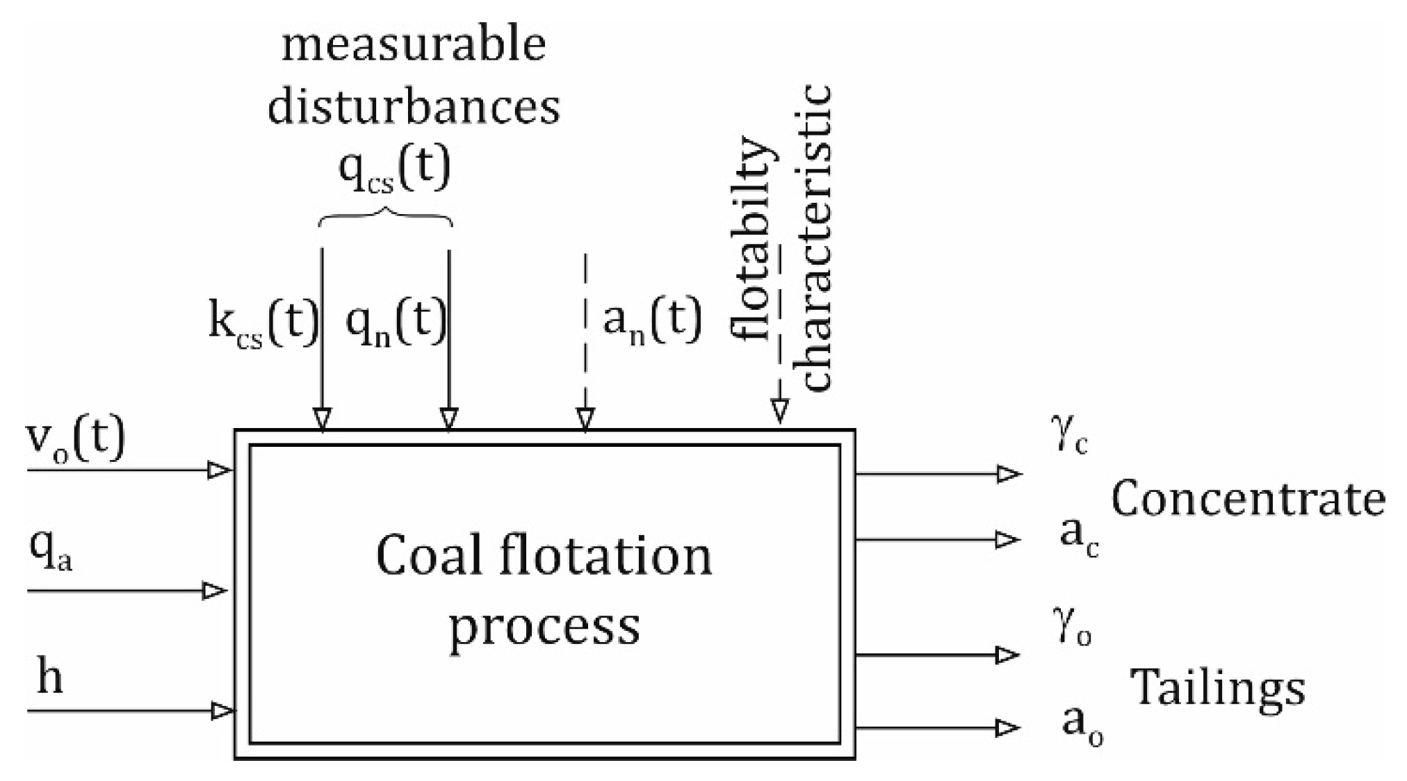
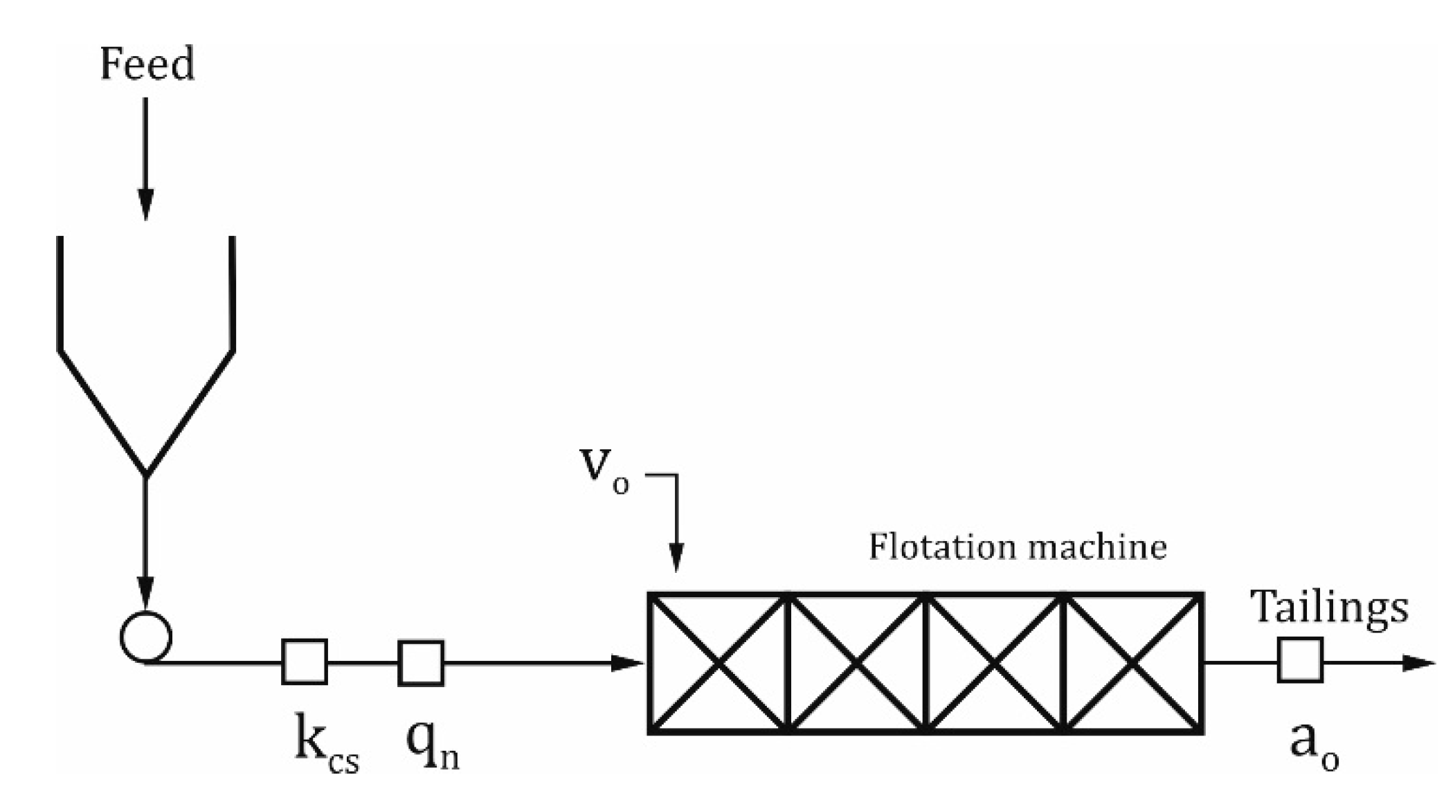
From the point of view of automatic control, the coal flotation process can be represented schematically as in Figure 1. It is a non-linear dynamic object with three control signals, namely flotation-reagent flow rate (v_o), turbidity aeration air flow rate (q_a), and suspended solids level in the flotation cell (h). The output volumes are concentrate outflow γ_k, ash content in concentrate a_k, and waste outflow γ_o, ash content in waste a_o. Since the physical and chemical conditions are mainly determined by the flotation reagents, the flotation-reagent flow rate can be considered as the leading control volume. This is all the more justified as the level of suspended solids in the flotation cell and the level of air flow rate are usually stabilized in local control loops and their setpoints are changed occasionally.

As already mentioned, the available output measure is the ash content of the tailings; therefore, the dynamic properties of the coal flotation process considered as a facility with the flow rate of the flotation reagent as an input and the ash content of the flotation tailings as an output signal are of interest. In the flotation process, the interfering signals are the parameters of the changing feed. 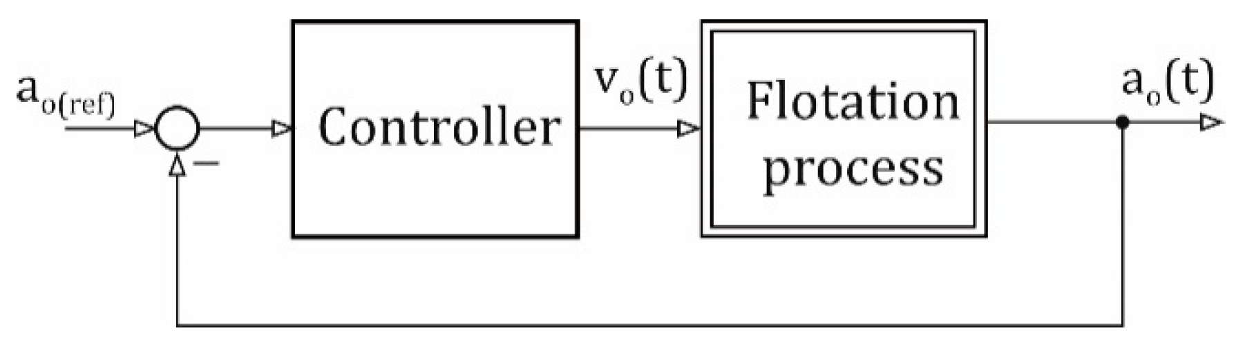As the results of industrial research have shown, the feed parameters can remain constant or change slightly over the next few operating periods (working shifts) [14,15]. This steady state of the feed can be used to determine interesting dynamic characteristics that can be used to estimate the parameters of the process-dynamics model. Knowledge of the dynamic properties of the flotation process makes it possible to determine the response time of the system to a change in the input signal (flotation reagents) at different parameters of the flotation feed, which is valuable information for the process operator. Knowledge of the dynamic model is essential for the selection of regulator settings in the situation of closing the feedback loop from the waste-ash signal. (Figure 2).

Due to the non-linear static characteristics of the coal flotation process, automatic control is only justifiable around a fixed operating point, and with each change in the operating point, identification of the dynamics model and adjustment of the controller settings should take place. This justifies the need to identify the dynamic properties of the process with the use of recursive methods, i.e., methods enabling the determination of the object model during its operation.. These include a method based on the Kalman filter equations [16]. This paper describes an algorithm with the use of the Kalman filter to identify an object model based on the response of the system in the form of a change in the ash content of the flotation tailings to a step in the flow rate of the flotation reagent as the leading control signal. The results of the identification of the dynamics model with the application of the Kalman filter were compared with the results of the batch method (least squares method), which was adopted as the reference method.

2. Method for Identifying the Dynamic Properties of the Coal Flotation Process

A step response method was used in an industrial experiment. It involves stepping an input signal and observing the system’s response to this step function. It is a well-known method that is one of the basic tests [17]. It usually provides sufficient accuracy without the need for lengthy and complex analyses. Identifying an object with this method involves conducting an experiment to collect data and calculating the parameters of the dynamics model. If the batch method is used, the model parameters are calculated after the experiment has been completed and the data collected, whereas if the recursive method is used, the model parameters are determined during the experiment (in real time). The step response method requires an arbitrary adoption of the structure of the dynamics model. For inertial industrial facilities, an inertial model of order one with a delay is often sufficient to describe the dynamic properties [17,18]. It is particularly useful for automatic process control and the associated selection of controller settings (Figure 2) [19]. The equation of the object model can be represented by the operator transmittance:

$$K\left(s\right)=\frac{k\times e^{-s\tau }}{sT+1}$$

(1)

where:

• k—gain, %/(dm³/h);
• T—substitute time constant of the object, s;
• τ—delay, s.

Equation (1) implies that the identification is reduced to determining the values of the parameters k_s, T_s, and τ_s. The adoption of Equation (1) to describe the dynamic properties of the coal flotation process is appropriate due to the inertial characteristic of the course of the ash content in the flotation tailings as a result of the step change in the amount of reagent fed and the transport delay that occurs in this process (flotation IZ-5).

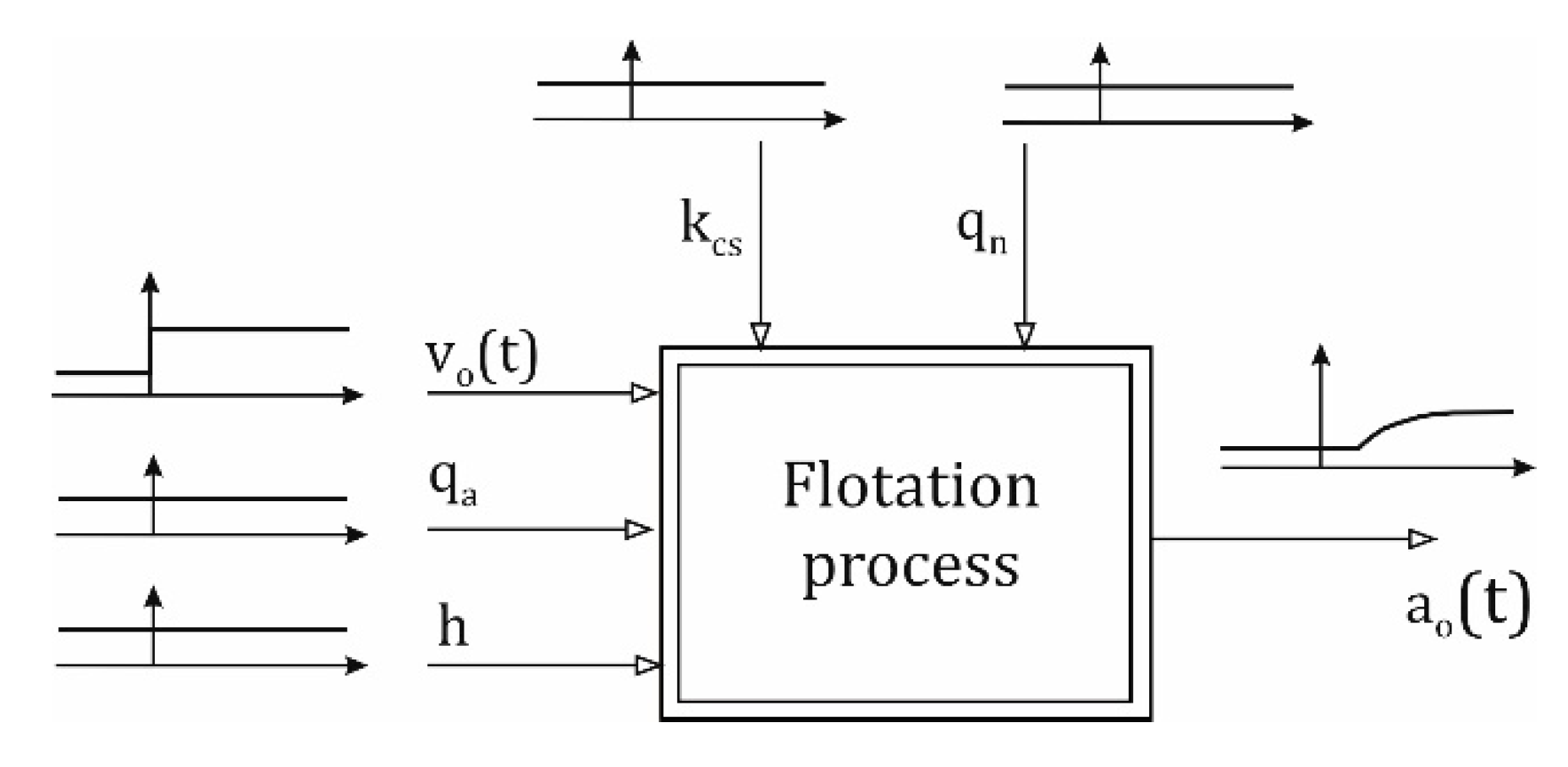
In the case of the coal flotation process, the identification experiment consists of a step change in the flow rate of the flotation reagent dosed into the system (from an initial value to a final value) and recording of the induced changes in the output signal (ash content of the flotation tailings), while keeping the other input quantities constant throughout the measurement experiment, as schematically shown in Figure 3. Due to the non-linearity of the static characteristics [20,21,22], when using this method, linearization is carried out when an object passes from one operating point to another as a result of a step change in the input signal (intensity of the flotation reagent). This consists in reducing the value of the excitation by its initial value and subtracting its initial value from the system response value in successive steps.

Owing to the discretely observed (every sampling period T_s) output signal, the dynamics of the object can be described by the equation:

$$y\left(i\right)=a\times y\left(i-1\right)+b\times u\left(i-m\right)$$

(2)

where:

• i—sampling step i = t/T_s;
• T_s—sampling period, s;
• y(i)—output signal (ash content of flotation tailings) observed discretely every sampling period y(i) = a_o(i) − a_o(0), %;
• u(i)—input signal (flow rate of flotation reagent) u(i) = v_o(i) − v_o(0), dm³/h;
• a, b—model coefficients;
• m—parameter related to delay.

The relationship of coefficients a, b, and m with parameters k, T, and τ is expressed in the equations:

$$T=-\frac{T_s}{\ln \left(a\right)}$$

(3)

$$k=\frac{b\times e^{\frac{T_s}{T}}}{e^{\frac{T_s}{T}}-1}$$

(4)

$$\tau =m\times T_s$$

(5)

Estimation of model parameters (1) requires:

-

Determination of coefficients a, b, and m;

-

Calculation of parameters k, T, and τ with the use of Equations (3)–(5).

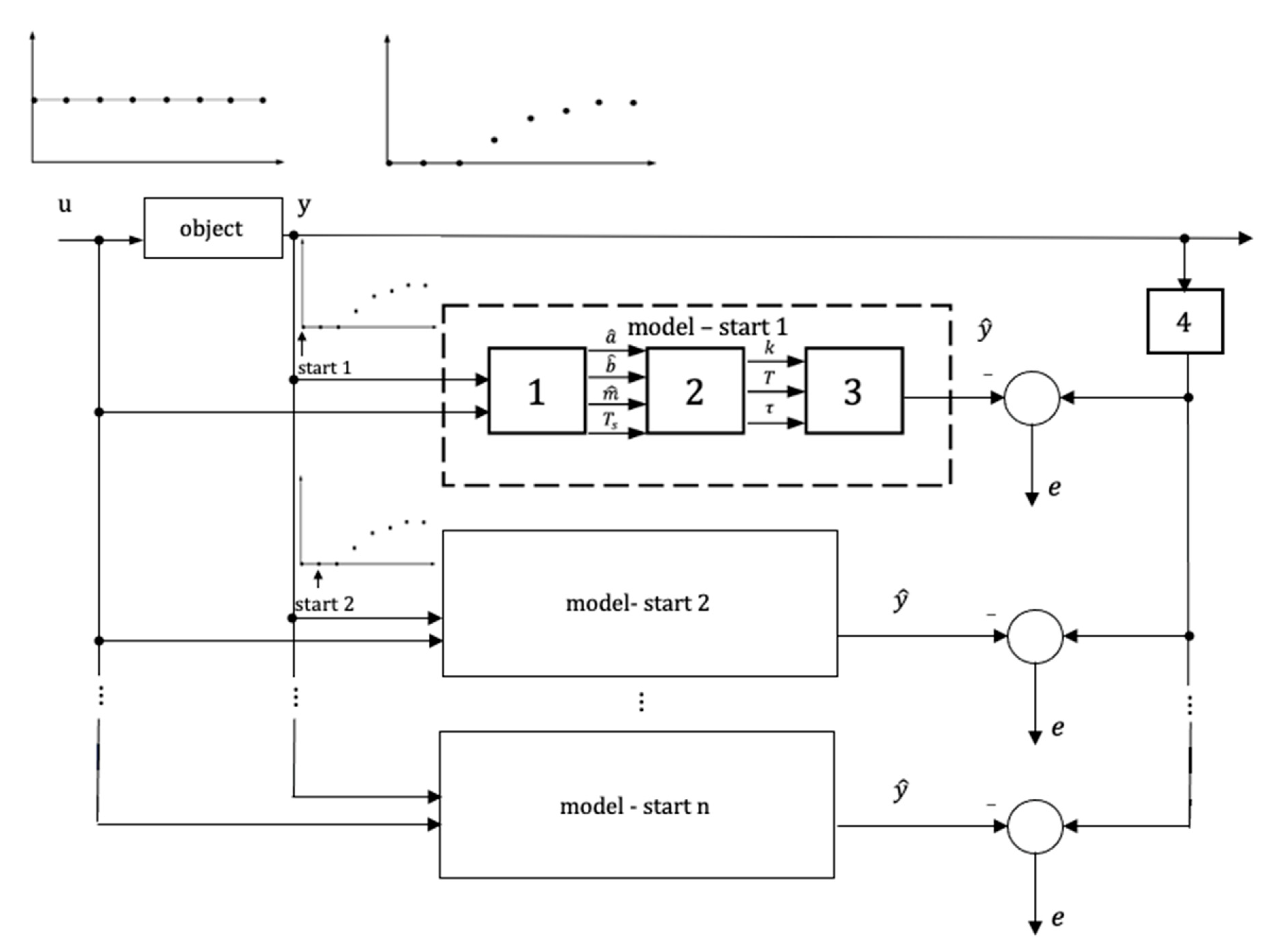
In the case of the method based on the Kalman filter, the determination of the time delay measure in the form of parameter m requires parallel estimation of the coefficients a and b, during the flotation process, with successive estimation starting every successive sampling period. This means that for time t = 0 the calculation of the first values of model parameters (2) begins, for time t = T_s the second, for time t = 2T_s the third, and so on. The calculation ends when the steady state occurs. The best model is assumed to be the one whose parameter values provide the best fit to the empirical data. Then, based on the knowledge of the parameters a, b, and m, parameters k, T, and 𝜏 can be determined. The principle of determining the delay 𝜏 and the model parameters with the use of Kalman filter is illustrated in Figure 4.

In the case of the reference method, the method of least squares, the delay is determined iteratively, whereby the data series must be complete and the calculations are carried out after the data have been collected. The calculation starts with all the empirical data from which the a and b values are determined. In the next iteration, the first sample of the step response is removed and the calculation is repeated. In subsequent iterations, the course of action is analogous. With this method, in each subsequent iteration, the step response data are reduced by one sample (starting from the first) and the parameters a and b are estimated. In this case, the delay measure m is the number of samples removed, and the best model is taken to be the one that provides the best fit to the empirical data.

3. Estimation of Model Parameters

3.1. Application of the Kalman Filter for the Identification of a Dynamics Model

Suppose an object is given with a first-order inertial element structure described by the equations [23,24]:

$$x\left(i\right)=a\times x\left(i-1\right)+b\times u\left(i-1\right)$$

(6)

$$y\left(i\right)=x\left(i\right)+z\left(i\right)$$

(7)

where:

• a, b—unknown, sought parameters of the equation;
• u—disturbance, which is a random variable with a normal distribution N(0,σ_z²).

The next moment (i + 1) in Equations (6) and (7) takes the form of:

$$x\left(i+1\right)=a\left(i\right)\times x\left(i\right)+b\left(i\right)\times u\left(i\right)$$

(8)

$$y\left(i+1\right)=x\left(i+1\right)+z\left(i+1\right)$$

(9)

By determining the state variable x(i) from Equation (7) and substituting into Equation (8) we obtain:

$$x\left(i+1\right)=a\left(i\right)\times y\left(i\right)-a\left(i\right)\times z\left(i\right)+b\left(i\right)\times u\left(i\right)$$

(10)

Then by inserting Equation (10) into Equation (9) the equation of output is obtained as follows:

$$u\left(i+1\right)=a\left(i\right)\times y\left(i\right)+b\left(i\right)\times u\left(i\right)+z\left(i+1\right)-a\left(i\right)\times z\left(i\right)$$

(11)

Assuming that w(I + 1) = z(i + 1) − a(i)z(i) may be saved:

$$y\left(i+1\right)=a\left(i\right)\times y\left(i\right)+b\left(i\right)\times u\left(i\right)+w\left(i+1\right)$$

(12)

With the assumption that the system is stationary, the parameters of equation a and b have the same values at any time, i.e., there is a(0) = a(1) … = a(i − 1) = a(i) = a(i + 1) = … and b(0) = b(1) … = b(i − 1) = b(i) = b(i + 1) = …. With the application of matrix notation

$$\theta ={\left[\begin{array}{cc}a& b\end{array}\right]}^T$$

(13)

and

$$V\left(i\right)=\left[\begin{array}{cc}y\left(i\right)& u\left(i\right)\end{array}\right]$$

(14)

the following set of vector-matrix equations can be introduced:

$$\theta \left(i+1\right)=\theta \left(i\right)$$

(15)

$$y\left(i+1\right)=V\left(i\right)\times \theta \left(i\right)+w\left(i\right)$$

(16)

The parameters of the matrix are constant at all times, as it is a matrix containing the sought values of the object model parameters (6) and (7), hence Equation (15) is legitimate. Consequently, Equation (15) can be treated as the equation of state, and Equation (16) then becomes the equation of exit. The estimation of the parameters $\widehat{\theta }\left(i+1\right)$ can be done with the use of Kalman filter equations, which take the following form:

$$\widehat{\theta }\left(i+1\right)=\widehat{\theta }\left(i\right)+K\left(i+1\right)\times \left(y\left(i+1\right)-V^T\left(i\right)\times \widehat{\theta }\left(i\right)\right)$$

(17)

$$K\left(i+1\right)=P\left(i\right)\times V^T\times {\left(V\times P\left(i+1|i\right)\times V^T+R\right)}^{-1}$$

(18)

$$P\left(i+1\right)=\left(I-K\left(i+1\right)\times V\left(i\right)\right)\times P\left(i\right)$$

(19)

where:

• P—error covariance matrix;
• K—Kalman gain;
• I—unit matrix.

As is visible in the Equations (11) and (12) disturbances at successive moments in time are correlated with each other. The variance of the disturbance w(i + 1) is ${\sigma }_z^2·\left(1+a^2\right)$. Equation (18) shows that in order to calculate the Kalman gain K, it is necessary to know the parameter a, which in turn is the quantity sought. Therefore, in the calculation algorithm, the parameter a should be replaced by its estimate at time iT_s:

$$R={\sigma }_z^2\cdot \left(1+{\widehat{a}}_1^2(i)\right)$$

(20)

The presented set of equations is a recursive Kalman filter that allows us to determine the parameters of Equation (6). It is one of the recursive online identification methods. Therefore, it can be used in real-time systems, e.g., for the selection of controller settings. The values of the sought parameters are calculated at any time on the basis of a pair of points (Equation (14)).

3.2. Least Squares Method

One of the batch methods, i.e., the method of least squares, was adopted as the reference method. It requires the collection of complete measurement data and then the calculation of the values of the sought-after coefficients of Equation (2) with the use of the estimator [25]:

$$\theta ={\left(C^{T}C\right)}^{-1}{C}^{T}Y$$

(21)

where:

• Y—object output observation matrix, Y = [y₁, …, y_N]^T;
• N—number of sampling points.

The matrix C contains both input and output quantities, which for the estimated parameters of model (1) can be saved:

$$C=\left[\begin{array}{cc}-y\left(0\right)& u\left(0\right)\\ ⋮& ⋮\\ -y\left(N-1\right)& u\left(N-1\right)\end{array}\right]$$

(22)

4. Results of the Identification of the Dynamic Properties of the Coal Flotation Process

4.1. Research Results

The identification was carried out on the basis of data recorded during an experiment at the industrial facility of a coal preparation plant of one of the Polish mines with a flotation machine of the IZ-5 type. A schematic diagram of the flotation industrial facility is shown in Figure 5.

The industrial facility was equipped with a measurement system that allowed for real-time measurement of the feed flow rate, the concentration of solids in the feed, and the ash content of the flotation tailings. The individual quantities were measured using an electromagnetic flow meter (q_n), a radiometric density meter (k_cs), and an optical ash meter (a_o), respectively. In the case of the experiment, recording was carried out with a sampling period T_s of 30 s and the length of the recorded data series was 53, corresponding to a time of 1590 s. The initial value of the reagent flow rate v_o(0) was 1.5 dm³/h and was stepped up to 7.5 dm³/h, meaning that the step increase in this quantity was u = 6 dm³/h. At the time of the step change v_o, the ash content of the flotation tailings (initial value a_o (0)) was 53.8%. During the measurement experiment, the feed parameters were monitored. They were found to be invariant over time, with values of q_n = 513 ± 2 m³/h and k_cs = 116.2 ± 1 kg/m³

The validity of the model was assessed using the mean-squared-error criterion expressed by the formula [26,27]:

$$MSE=\frac{1}{N}{\displaystyle \sum }_{i=1}^N{\left(e\right)}^2=\frac{1}{N}{\displaystyle \sum }_{i=1}^N{\left(y-\widehat{y}\right)}^2$$

(23)

where:

• e—the rest of the model, %.

The value of the mean squared error is determined for the model identified by the recursive method (the Kalman algorithm), and the least squares method, adopted as the reference method. On the basis of the quantitative evaluation of criterion (23), the model better fitted to the empirical data should be considered the one for which the value of the mean squared error is smaller.

4.2. Identification Results

The results of the identification of dynamic models of the coal flotation process with one control input in the form of the flow rate of the flotation reagent and one output—the ash content in flotation tailings, obtained with the use of the Kalman algorithm, are summarized in

Table 1. Results of the identification of the dynamic properties of the hard coal flotation process.

Method	m	a	b	τ (s)	k	T (s)	MSE (%2)
KF	4	0.8925	0.3561	120	3.3126	263.8	10.79
	5	0.8879	0.3600	150	3.2119	252.3	7.13
	6	0.9004	0.3054	180	3.0674	286.1	2.69
	7	0.8966	0.3535	210	3.4201	275.0	6.01
	8	0.8292	0.5750	240	3.3665	160.2	12.35
	9	0.7656	0.7721	270	3.2943	112.3	13.73
LS	7	0.8975	0.3087	210	3.0114	277.4	2.36

KF—recursive identification method with the use of the Kalman algorithm, LS—least squares method.

. Examples of the waveforms of the step response of the identified dynamic models and the waveforms of the determined parameters of Equation (2) are shown in Figure 6 and Figure 7.

The step response waveforms presented in Figure 6, calculated on the basis of the identified dynamic models, show that the use of an approximation using a first-order model with a delay is justified, as it is clearly evident in the first moments that the object does not respond (no change in the ash content of the flotation tailings) to an excitation signal in the form of a step change in the amount of reagent dosed to the process.

In the waveforms of the estimation of the parameters of the dynamic model of Equation (2) shown in Figure 7, one can see, in each case, the moment of the start of the identification process resulting from the delay m (start 1, start 2, … from Figure 4). One can also see there the determination of the values of the parameters a and b in the dominant majority of cases. This shows that the time of recording and therefore of calculation was sufficient.

The optimum values, in terms the adopted parameters m, a, and b, as the results summarized in Table 1 show, were obtained for delay 𝜏 = 180 s. For this value of delay, the calculated remaining parameters of the operator transmittance described by Equation (1) in the form of the gain k and the equivalent time constant of the object T are 3.3 and 286 s, respectively. Comparing the identification results of the method with the use of the Kalman filter with the optimum model obtained for the reference method (LS), it can be seen that both the estimated parameters and the values of the MSE criterion for both cases have similar values. A graphical comparison of the response of both models to the step function (Figure 8), i.e., determined by the least squares method and the Kalman algorithm, seems to confirm the observation of a significant convergence of the obtained results. This shows that the method with the use of the Kalman filter can be useful in modeling the dynamic properties of flotation for the purpose of automating this process.

5. Discussion

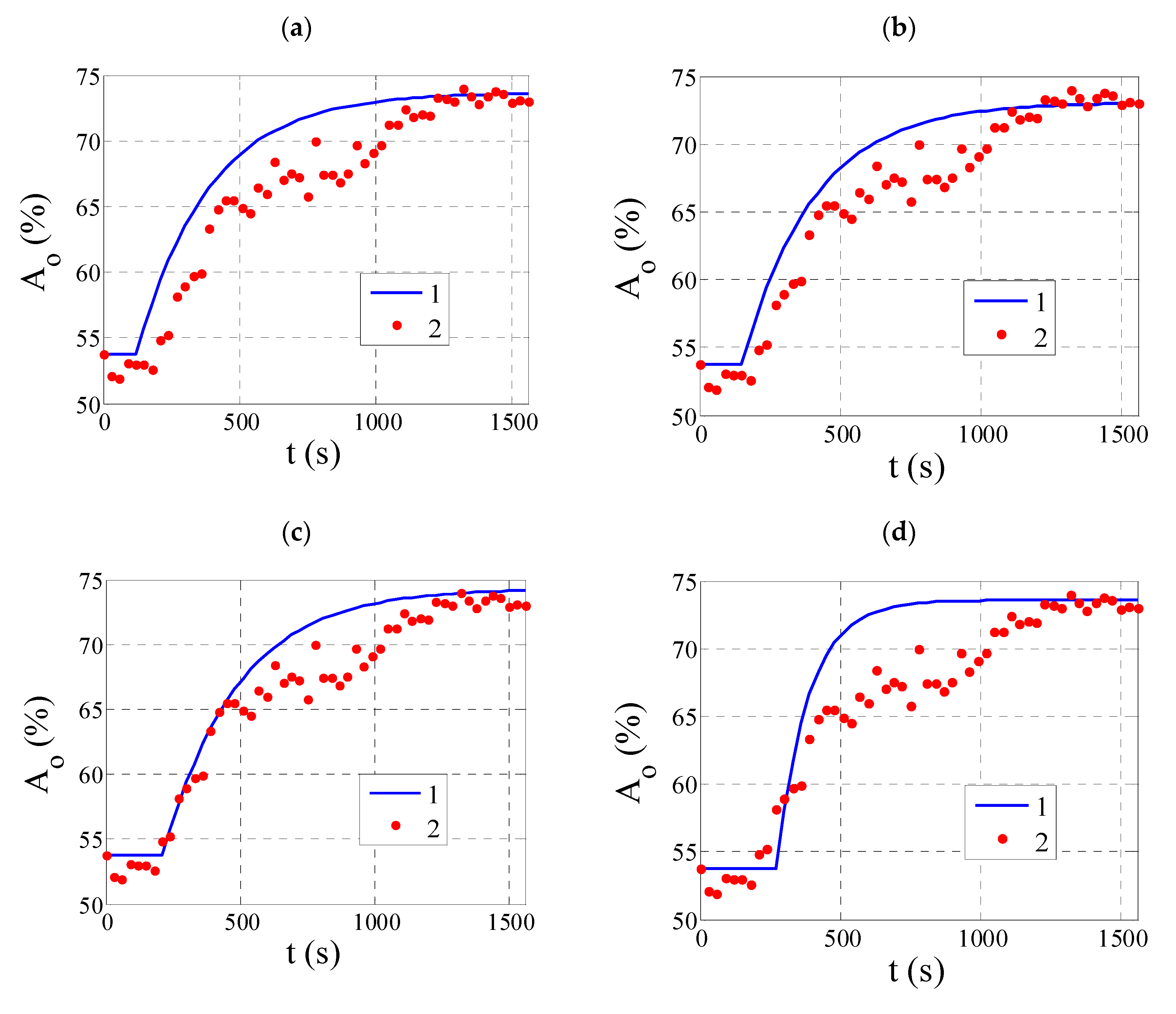
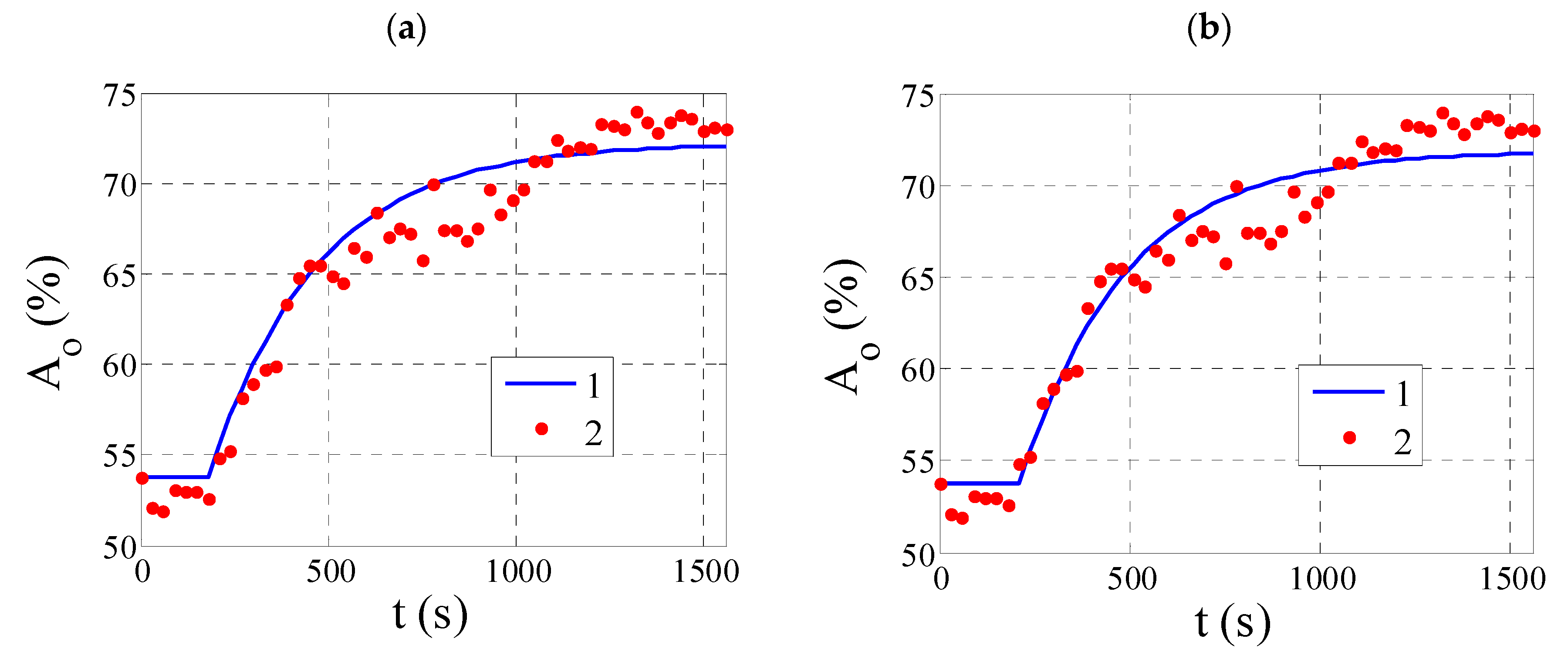
The calculations carried out show that the approximation of the step response of the coal flotation process using a first-order inertial element structure model with a delay gives satisfactory results. On the basis of a comparative analysis of the obtained results, it can be concluded that the dynamic model calculated by the recursive method, using the Kalman filter, shows a similar fit to the empirical data, in terms of the adopted index (MSE = 2.7), as the model determined by the least squares method (MSE = 2.4). The parameters of Equation (2), and therefore also of model (1) estimated by the KF method, have values close to the results of identification by the least squares method. The experiment and identification calculations resulted in coefficients of Equation (2) with values a = 0.9004, b = 0.3054, and m = 6 for the Kalman filter method and a = 0.8975, b = 0.3087, and m = 7 for the reference method, i.e., the least squares method. These coefficients correspond to parameter values T = 286.1 s, k = 3.0674, and 𝜏 = 180 s for the KF method and T = 277.4 s, k = 3.0114, and 𝜏 = 210 s for the least squares method. For the optimum, in the sense of Equation (23), of the model determined by KF, the value of the time constant is about 9 s longer than for the reference method, which is only about 3% of the value of T, determined by the LS method. On the other hand, the static gain k estimated with the use of the KF method has a value about 0.06 higher than the result of the identification with the LS method, which is about 2% of the value obtained with the reference method. The greatest difference in the value of the model parameter (1) occurs for τ. The value of the delay determined with the use of the Kalman filter is 30 s shorter than the value of this parameter estimated with the least squares method (in an iterative manner), and this represents approximately 15% of the reference value. This difference is due to the fact that the delay calculated by both methods is a multiple of the sampling period, so in the case under consideration, the difference in values calculated using the KF and LS methods corresponds to the smallest possible deviation, i.e., the sampling period T_s.

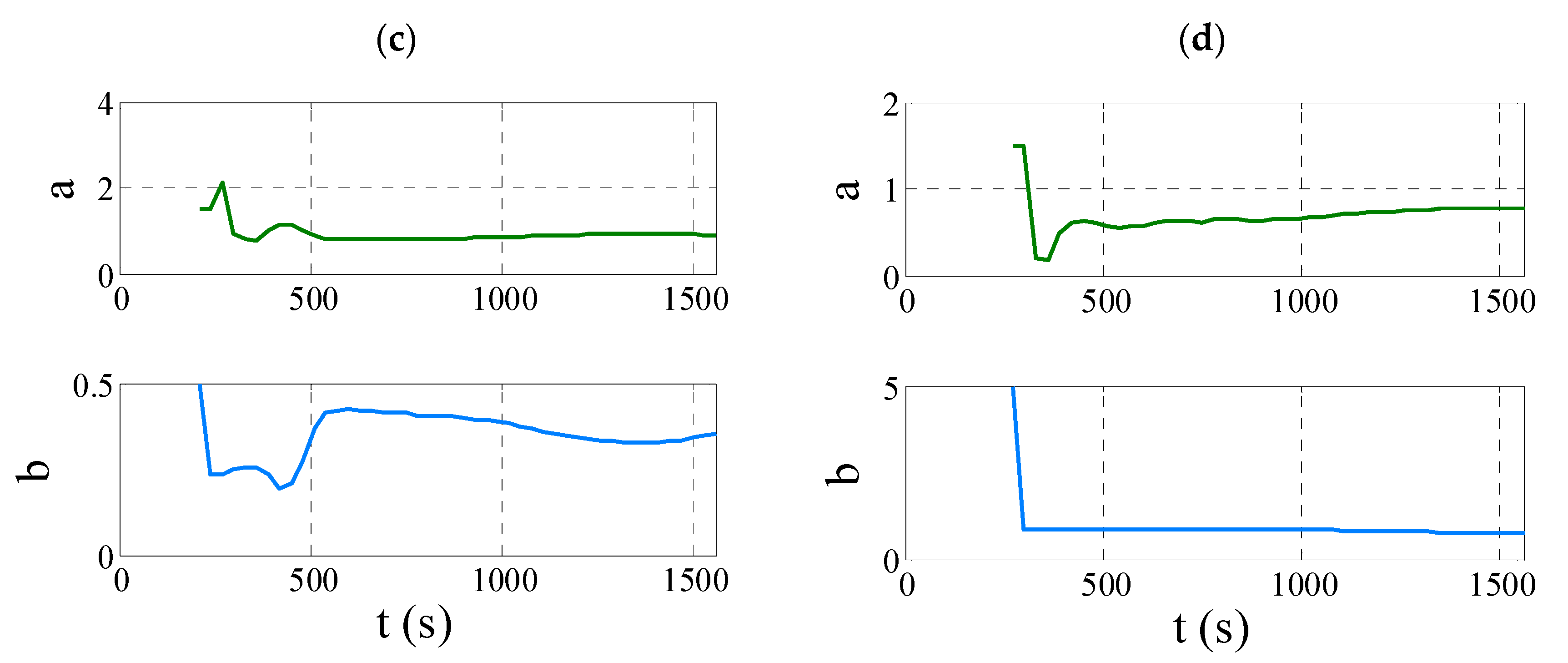
Analysing the other results summarized in Table 1, one may see that for 𝜏 = 210 s the difference in the values of the parameters a estimated using the Kalman filter—based method and the reference method (LS)—is negligible. This translates directly into the values of the time constants T, which are 275.0 s and 277.4 s, respectively. 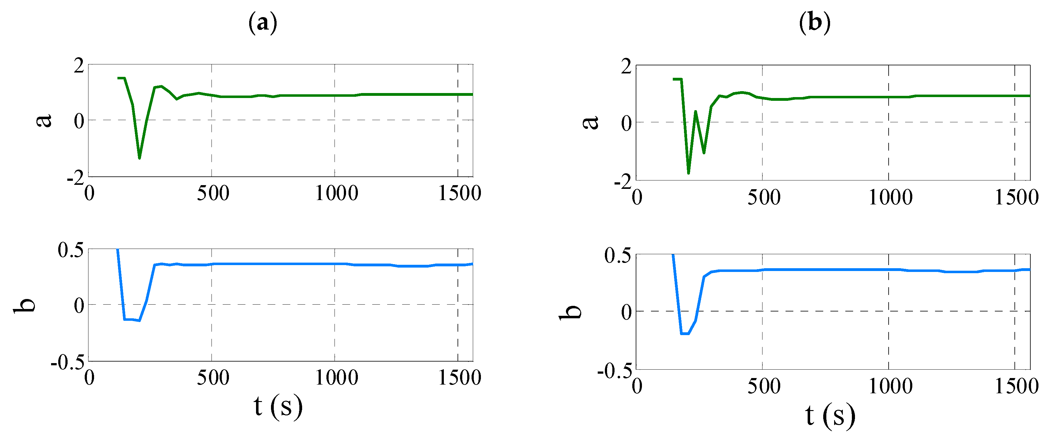In this case, however, the difference in the values of the parameter b is not negligible, as it leads to an overestimation of the gain k to the disadvantage of the KF method. The waveforms of the continuously identified coefficients a and b, shown in Figure 7c, (when 𝜏 = 210 s) show that the values of these parameters have not settled. This may be indicative of insufficient computation time, and hence experimental time, required to achieve the final result, which, in turn, may have been the cause of the incorrect value of the coefficient k. It seems that extending the experimental time in this otherwise isolated case could have had a beneficial effect on the final result. However, it should be emphasized that this problem did not occur in any of the other cases, and the identified parameters a and b with the use of the Kalman filter have always reached the set values (Figure 7).

Evaluating the other results of the identification of the parameters of model (1) for times 𝜏 shorter than 210 s, it can be concluded that the values of the gains k and the time constants T are comparable. On the other hand, it is noted that the dynamic error ${\left(y-\widehat{y}\right)}^2$ occurring in the time interval corresponding to the three time constants, counting from the time equal to the delay, is the larger the shorter 𝜏 is. On the other hand, for the cases of estimated parameters of the model (1) with the KF method, when the delay is longer than 210 s, a shortening of the equivalent time constants is observed (the longer 𝜏 is, the shorter T is), which directly translates into an increase in the value of the MSE criterion.

6. Conclusions

The results of the identification studies show that the dynamic properties of a coal flotation object with one control input (v_o) and one measurement output (a_o) can be presented as first-order inertial element models with delay, regardless of the identification method used (KF or LS). Based on a comparative analysis of the results, it can be concluded that the application of the Kalman filter method for the identification of dynamic models of a coal flotation object with one input v_o and one output a_o, yields results comparable to those obtained by the least squares method. It should be noted that the values estimated with both methods are similar and the step characteristics converge significantly (Figure 8). A slightly lower criterion value was obtained using the reference method (MSE = 2.4) comparing to the KF method (MSE = 2.7). It is possible to conclude that, in terms of the criterion adopted, the least squares method produced a slightly better model than the method based on the Kalman filter. However, it should be noted that the reference method is an off-line batch method, so in the case of the model identification (1), based on the step response, it requires the collection of all data and iterative actions using the vector-matrix Equation (21). In contrast, the dynamic model identification method with the use of the Kalman filter offers the possibility of estimating the parameters of the dynamic models of the flotation process on the on-going basis (in discrete moments of time). It is a recursive algorithm, and therefore there is no need to store the full data series for recalculation at each successive step. Due to the recursive nature of the Kalman filter method and the fact that the method produces results very close to those of the reference method, it should be emphasized that it is computationally advantageous. This is of particular importance when the method is to be used in real time to select controller settings in an automatic flotation process control situation. This is all the more so because, due to the non-linear nature of coal flotation as a control object and the random disturbances of the changing feed, the identification process has to be repeated periodically. Due to its advantages, the Kalman filter identification method can be of application in the field of coal flotation process identification for control purposes. The conducted research may indicate to other researchers that it is beneficial to use the Kalman filter method to identify coal flotation for highly sensorized systems controlling this process in processing plants in other countries.

A novelty is the use of the method based on the Kalman filter, which is a recursive algorithm, and therefore does not require the storage of full data series for their conversion in each subsequent step. Thus, it will not burden the control unit, and the identification procedure itself may run periodically (repeated) for the purpose of checking the values of the estimated model parameters, and consequently adjusting the controller settings. This should be done after changing the feed parameters such as the solids concentration or the feed flow rate.

References

1. Majumder, A.K.; Barnwal, J.P. Processing of coal fines in a water-only cyclone. Fuel 2011, 90, 834–837. [Google Scholar] [CrossRef]
2. Niu, C.; Xia, W.; Li, Y.; Bu, X.; Wang, Y.; Xie, G. Insight into the low-rank coal flotation using amino acid surfactant as a promoter. Fuel 2022, 307, 121810. [Google Scholar] [CrossRef]
3. Fečko, P.; Janakova, I.; Raclavska, H.; Tora, B. Application of flotation in the decontamination of sediments from the Cerny prikop stream. Pol. J. Chem. Technol. 2009, 11, 8–11. [Google Scholar] [CrossRef] [Green Version]
4. Liao, Y.; Yang, Z.; An, M.; Cao, Y.; Hao, X.; Song, X.; Chen, L. Spreading behavior of dodecane-oleic acid collector mixture in low-rank coal flotation. Fuel 2022, 308, 122071. [Google Scholar] [CrossRef]
5. Augustyn, A.R.; Pott, R.W.; Tadie, M. The interactions of the biosurfactant surfactin in coal flotation. Colloids Surf. A Physicochem. Eng. Asp. 2021, 627, 127122. [Google Scholar] [CrossRef]
6. Zhu, H.; Zhu, J.; Min, F.; Valdivieso, A.L.; Arroyo, M.A.C.; Wang, H. Effect of frother addition mode on coal flotation in downflow flotation column. J. Clean. Prod. 2021, 278, 123844. [Google Scholar] [CrossRef]
7. Cierpisz, S.; Cierpisz, T.; Król, S.; Joostberens, J.; Piwowar, E. Automatic regulation of the coal flotation process in the coal preparation plant of the Sosnica mine. MINING Inform. Autom. Electr. Eng. 1999, 7, 7–14. [Google Scholar]
8. Clarkson, C.; Hornsby, D.; Walker, D. Automatic Flotation Control using On-Stream Ash Analysis. Coal Prep. 1993, 12, 41–64. [Google Scholar] [CrossRef]
9. Laurila, M. The Use of On-Line Coal Ash Monitoring System in Local Control Applications. Coal Prep. 1994, 14, 81–91. [Google Scholar] [CrossRef]
10. Sikora, T. Control—Measuring systems and devices for coal preparation plants. Inżynieria Miner. J. Pol. Miner. Eng. Soc. 2000, 2, 41–46. [Google Scholar]
11. Astafieva, I.M.; Gerasimov, D.N.; Makseev, R.E. Density measurement by radiometric method with gamma irradiation from sources of low activity. J. Phys. Conf. Ser. 2017, 891, 012322. [Google Scholar] [CrossRef]
12. Smyła, J. Ash Meters in the Automation of Froth Flotation of Coal. In Proceedings of the XV International PhD Workshop OWD 2013, Wisła, Poland, 19–22 October 2013; pp. 419–423. [Google Scholar]
13. Joostberens, J. Application of fuzzy modelling based on experts’ knowledge for modelling a coal flotation process. MINING Inform. Autom. Electr. Eng. 2010, 3, 5–15. [Google Scholar]
14. Joostberens, J.; Rybak Au Pielot, J.; Dylong, A. Application of the ARMA Model to Describe and Forecast the Flotation Feed Solids Flow Rate. Energies 2021, 14, 8587. [Google Scholar] [CrossRef]
15. Joostberens, J. Modeling of Solids Concentration in The Feed For Coal Flotation. Gospod. Surowcami Miner. Miner. Resour. Manag. 2014, 30, 55–66. [Google Scholar]
16. Kalman, R.E. A New Approach to Linear Filtering and Prediction Problems. Trans. ASME J. Basic Eng. 1960, 82, 35–45. [Google Scholar] [CrossRef] [Green Version]
17. Rake, H. Step Response and Frequency Response Methods. Automatica 1980, 16, 519–526. [Google Scholar] [CrossRef]
18. Kaula, R. Sensitivity problems of the coal flotation process control system. Gospod. Surowcami Miner. Miner. Resour. Manag. 2018, 34, 83–96. [Google Scholar]
19. Astrom, K.J.; Hagglund, T. Revisiting the Ziegler–Nichols step response method for PID control. J. Process Control. 2004, 14, 635–650. [Google Scholar] [CrossRef]
20. Cierpisz, S.; Joostberens, J. Charakteriststics of the Coal Floatation Process in Control Circuit; IX Balkan Mineral Processing Congress (IX BMPC): Istambul, Turkey, 2009; pp. 11–16. [Google Scholar]
21. Cierpisz, S.; Joostberens, J. Simulation of fuzzy control of coal flotation. IFAC Proc. Vol. 2006, 39, 210–214. [Google Scholar] [CrossRef]
22. Kalinowski, K.; Kaula, R. Determination of static characteristics of flow flotation machines based on experiments of the kinetics of the batch coal flotation. Arch. Min. Sci. 2016, 61, 47–57. [Google Scholar] [CrossRef] [Green Version]
23. Urrea, C.; Agramonte, R. Kalman filter: Historical overview and review of its use in robotics 60 years after its creation. J. Sens. 2021, 2021, 9674015. [Google Scholar] [CrossRef]
24. Sun, Y.; Xie, J.; Guo, J.; Wang, H.; Zhao, Y. A Modified Marginalized Kalman Filter for Maneuvering Target Tracking. In Proceedings of the 2nd International Conference on Information Technology and Electronic Commerce, Zurich, Switzerland, 14–15 June 2014; pp. 107–111. [Google Scholar]
25. Wang, X.; Liu, X.; Chen, L.; Hu, H. Deep-learning damped least squares method for inverse kinematics of redundant robots. Measurement 2021, 171, 108821. [Google Scholar] [CrossRef]
26. Wang, J.; Chen, P.; Zheng, N.; Chen, B.; Principe, J.C.; Wang, F.Y. Associations between MSE and SSIM as cost functions in linear decomposition with application to bit allocation for sparse coding. Neurocomputing 2021, 422, 139–149. [Google Scholar] [CrossRef]
27. Ren, J.; Zhang, M.; Yu, C.; Liu, Z. Balanced MSE for Imbalanced Visual Regression. In Proceedings of the IEEE/CVF Conference on Computer Vision and Pattern Recognition, New Orleans, LA, USA, 18–24 June 2022; pp. 7926–7935. [Google Scholar]
Figure 1. Coal flotation process as a facility with multiple inputs and multiple outputs.
Energies 15 07926 g001
Figure 2. System for automatic stabilisation of ash content in flotation tailings.
Energies 15 07926 g002
Figure 3. Identification of a dynamic model of the coal flotation process with the use of the step response method.
Energies 15 07926 g003
Figure 4. Idealized block diagram of a method for identifying the dynamic properties of the coal flotation process with the use of Kalman filter. 1—estimation of the coefficients of Equation (2) with the use of Kalman algorithm, 2—block for converting the coefficients of Equation (2) into model parameters (1), 3—block for determining the step response of the model, and 4—block for recording the signal y during the measurement experiment.
Energies 15 07926 g004
Figure 5. Industrial facility for the coal flotation process.
Energies 15 07926 g005
Figure 6. The response of the ash content of the flotation tailings to a step change in the flow rate of the flotation reagent (from a value of 1.5 dm3/h to 7.5 dm3/h). 1—object output values determined on the basis of identified dynamic models by the method with the use of Kalman filter and 2—measured data for delay times (a) 120 s, (b) 150 s, (c) 210 s, and (d) 270 s.
Energies 15 07926 g006
Figure 7. Parameters of dynamic models with step responses as in Figure 6 estimated by the Kalman filter method for delay times (a) 120 s, (b) 150 s, (c) 210 s, and (d) 270 s.
Energies 15 07926 g007aEnergies 15 07926 g007b
Figure 8. Results of the identification of the dynamic properties of the coal flotation process in terms of the response of the models to the step function (1) against empirical data (2), determined with the use of (a) the Kalman filter and (b) the least squares method.
Energies 15 07926 g008