Article

A Current Sensorless Control of Buck-Boost Converter for Maximum Power Point Tracking in Photovoltaic Applications

1
Laboratory of Electrical Engineering and Renewable Energies LGEER, Electrical Engineering Department, University of Hassiba Ben Bouali Chlef, Chlef 02000, Algeria
2
Power Electronics and Renewable Energy Research Laboratory (PEARL), Department of Electrical Engineering, University of Malaya, Kuala Lumpur 50603, Malaysia
3
Electrical Engineering Department, University of Echahid Hamma Lakhdar El Oued, El-Oued 39000, Algeria
4
Electrical Engineering Department, University of Batna 2, Batna 05078, Algeria
5
School of Science, Computing and Engineering Technologies, Swinburne University of Technology, Hawthorn, VIC 3122, Australia
6
Department of Electrical Engineering, College of Engineering, Universiti Tenaga Nasional, Kajang 43000, Malaysia
*
Authors to whom correspondence should be addressed.
Energies 2022, 15(20), 7811; https://doi.org/10.3390/en15207811
Submission received: 8 September 2022 / Revised: 4 October 2022 / Accepted: 18 October 2022 / Published: 21 October 2022
(This article belongs to the Special Issue Advanced Research on the Control of Power Converters)

Abstract

:
In the present paper, a current sensorless (CSL) method for buck-boost converter control is proposed for maximum power point tracking (MPPT) photovoltaic applications. The proposed control scheme uses the mathematical model of the buck-boost converter to derive a predefined objective function for the MPPT control. The proposed scheme does not require any current sensor and relies only on the input voltage signal, which decreases the implementation cost. The proposed method is successfully implemented using a Matlab/Simulink/Stateflow environment, and its effectiveness is compared over the perturb and observe (P&O) method. An experimental rig, that includes a buck-boost converter, a PV simulator, and a resistive load, is used for the experimental validation. A rapid Arduino prototyping platform is used for the digital implementation, where the SAM3X8E microcontroller of the Arduino DUE board, which integrates an ARM Cortex-M3 MCU, is used as a target hardware for the proposed model-based controller developed under the Stateflow environment. Furthermore, the integrated pulse width modulation (PWM) macrocell is used to generate accurate PWM gate-drive signals for the buck-boost converter. Compared to the P&O, the presented simulation and experimental results show that the proposed method has reduced the computation burden and the sensor cost of implementation by 24.3%, and 27.95%, respectively.

1. Introduction

In the past decade, the world has faced huge challenges in terms of fluctuations in the cost of fossil fuels such as petroleum and natural gas, along with exhaustion and future shortages of these reserves, which has raised concerns about future energy supply [1]. From the available renewable energy sources, photovoltaic energy is one of the most important alternative solutions to ensure clean electricity production and cater to the pollution problems associated with conventional electricity generation methods. However, a high cost of implementation is one of the main challenges for the big-scale applications of photovoltaic (PV) generation systems [2]. In addition, the generated power from PV systems is extremely sensitive to environmental changes, such as solar irradiance and temperature. The integration of the maximum power point (MPP) tracker is compulsory to guarantee that the available power, which is produced from PV panels, is extracted effectively [3]. In the literature, conventional techniques are proposed to ensure the MPPT task under uniform insolation conditions, such as hill-climbing (HC) [4], constant voltage (CV) [5], perturb and observe (P&O) [3,6], and increment conductance (IncCond) [7,8], are the most prominent because their simplicity and ease of implementation. Over the last few years, several researchers have sought to improve the efficiency of photovoltaic systems using more complex algorithms inspired from the non-linear control theory, such as predictive-based MPPT [9], sliding mode control (SMC) [10], or using soft computing approaches, such as fuzzy logic control (FLC) [11], artificial neuron network (ANN) [12,13], flower pollination algorithm (FPA) [14], and deep learning (DL) [15]. These methods are appropriate for solving complex problems such as partial shading conditions, where the global maximum power point (GMPP) needs to be located accurately in a rapid manner [12,16]. Despite the outstanding results obtained using such techniques, they are complex and require advanced programming levels for their practical implementation. Besides, a high-performance calculator, such as a digital signal processor (DSP) or a field-programmable gate array (FPGA), is required for real-time implementation, making them unattractive for PV applications where the cost is a crucial factor, such as water pumping or solar lighting PV systems. In such applications, the array is composed of a number of panels and is rarely subjected to partial shading conditions. Therefore, since there is no need to implement complex MPPT algorithms, the cost of implementation can be reduced by implementing simple MPPT algorithms using rapid microcontrollers. Among them, the open-source Arduino rapid prototyping platform is being used recently as a tool for hardware implementation of various types of MPPT with different complexity levels. Table 1 lists several works that have used the Arduino platform for MPPT implementation. Recently, Matlab has added a package toolbox for a wide range of microcontrollers available in the market, enabling them to be a target hardware for developed model-based controllers under Simulink. Thus, more complex algorithms developed in a Simulink environment can be easily compiled and loaded into rapid microcontrollers. For example, the fuzzy logic was successfully implemented as an MPPT controller for the PV system using the Atmega2560 microcontroller running at a 16 MHz clock speed [17].
Conventional perturbative MPPT methods still require information on both current and voltage signals to perturb the operating point in the correct direction. Low-cost voltage sensing can be made by simply using a voltage divider [18]. However, safe current sensing requires usually costly isolation circuits to protect the control board. To avoid the use of a current sensor in MPPT, several methods were proposed based on different approaches. Authors in [21] proposed a voltage-sensor based MPPT controller using a boost converter with direct duty cycle control. In this approach, an optimization function that has derived from the mathematical model of the converter is utilized. A similar concept was proposed [18] for the objective of reducing the computation time and the cost of implementation while improving the steady-state performance as well. The objective function used to track the MPP is derived from the SEPIC converter mathematical equations. The duty cycle can be directly updated using the objective function equation without the need for any other control loop. The algorithm improves the steady-state behavior by using adaptive step-size and avoid the drift issue in case of a fast increase in irradiance. In a separate work [20], the same authors proposed an indirect MPPT control scheme where the voltage sensor-based MPPT is implemented through a proportional-integral (PI) voltage controller. In work [22], a model predictive controller is used to observe the PV current. Although the current sensor is eliminated, the algorithm requires two voltage sensors for the measurement of the PV and output capacitor voltages. In another work [23], a voltage-based MPPT controller is developed using the mathematical model of an intermediate double boost (IDB) dc-dc converter. A single voltage-sensor MPPT using ANN was proposed in [24]. In this method, the database used for the ANN training is obtained by recording the behavior of a single voltage sensor algorithm based on a predefined objective function.
Although the operating area of the buck-boost converter is the full I-V plane regardless of the load value [25], there is no attempt yet made to propose a voltage-based sensor MPPT using the buck-boost converter. Within this context, the main contribution of this work is firstly to propose a simple and easy way to implement the current sensorless (CSL) MPPT algorithm for buck-boost converters. The second is to present a novel way for the hardware validation of Stateflow model-based controllers using a rapid prototyping platform through the Simulink support package for Arduino hardware. Thus, the proposed approach is developed using the Stateflow tool and is validated under a Matlab/Simulink environment. Then, the proposed algorithm is experimentally validated using an Arduino DUE microcontroller board.
The rest of this paper is arranged as follows: Section 2 presents the system under study and the mathematical model of its components. Section 3 describes the steps to be followed to derive the objective function from the mathematical model of the buck-boost converter. The objective function is the key element for the proposed CSL-MPPT algorithm and the Stateflow chart of the proposed CSL algorithm. Section 4 presents the results of the comparative study among the proposed CSL algorithm and the P&O algorithm obtained via simulation under a Matlab/Simulink environment. The hardware implementation of the Stateflow-based CSL algorithm using the rapid Arduino prototyping platform along with the experimental results are presented in Section 5. The conclusion is presented in the last section.

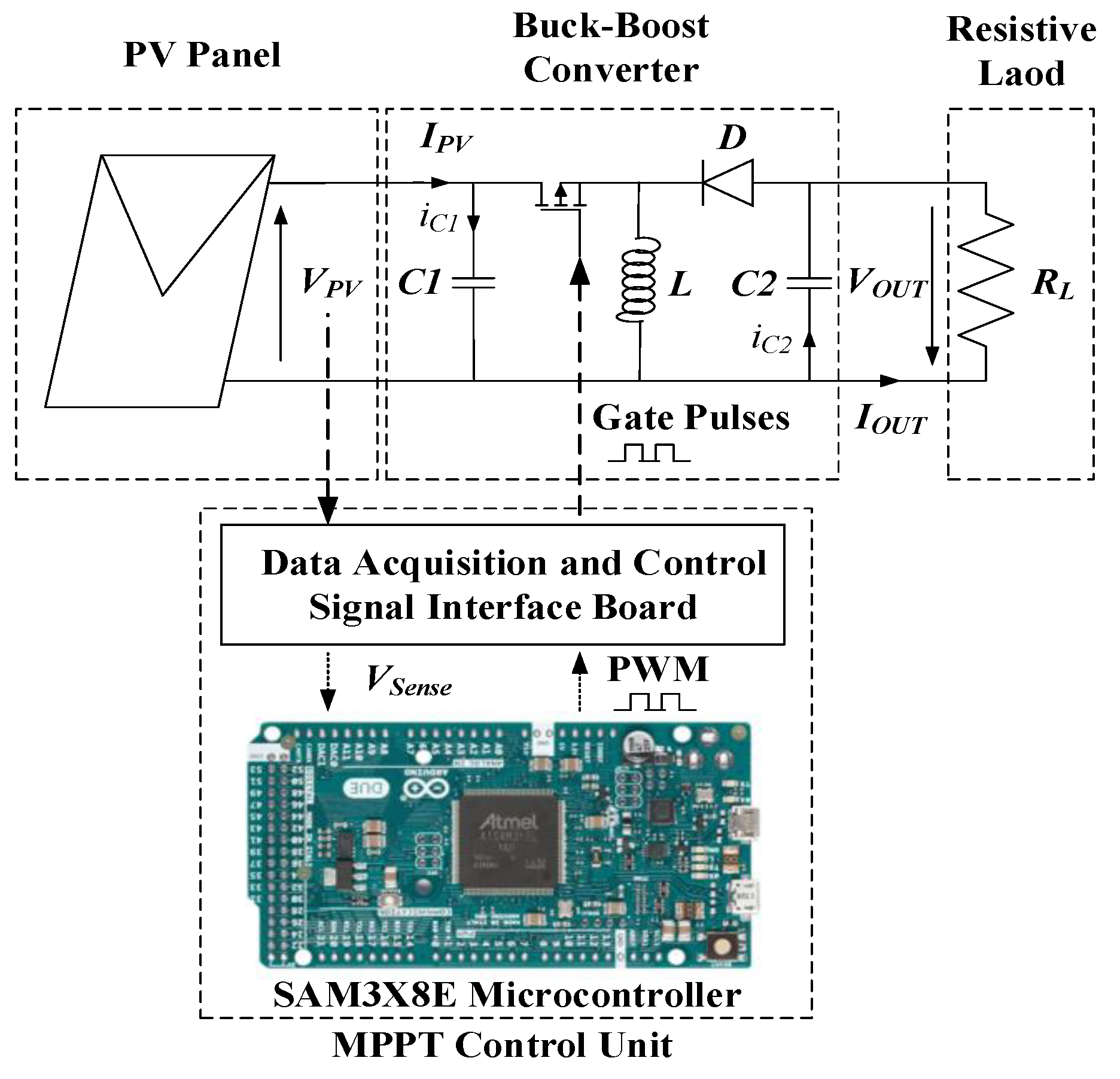
2. The PV System under Study

Figure 1 shows the topology for the PV system under study with the proposed CSL-MPPT digital controller. The power transformation process from the source (PV panel) to the load (resistive load) is connected through the buck-boost converter. The buck-boost is chosen since it has the capacity to work as a step-up/step-down converter, and it has the capacity to work in the maximum operating range of the I-V plane [12,26,27]. The MPPT digital controller keeps adjusting the PWM duty cycle of the power converter to ensure the operation at the maximum power point (MPP).
Figure 2 illustrates the circuit diagram of the equivalent one diode model of the PV cell [28]. The output voltage of the PV cell and the total current of the PV panel (I) can be obtained as follows:
V = R s h ( I p h I D I ) R s I
I = I p h I r s e q ( V + I R s ) N S n k T 1 V + I R s R s h
where Iph is the photocurrent, ID is given by the Schockley equation, which defines the I-V characteristic of an ideal diode, Rsh and Rs are the shunt and series resistances, respectively.
NS is the cells connected in series, Irs is the diode reverse saturation current, n is the diode ideality factor, q is the electron charge, T is the temperature of the p-n junction, and k is the Boltzmann’s constant.

3. The Proposed Current Sensorless MPPT Algorithm

3.1. Establishment of the Objective Function from the Mathematical Model of the Buck-Boost Converter

The key element of the proposed CSL-MPPT algorithm is annulling the objective function (Q) so that the operating point can be operated at the MPP. The procedure to establish the mathematical formula of Q is described hereafter:
The formula between the input and output voltage of the buck-boost is determined as follows:
V o u t = D 1 D V P V
where Vout, V P V ,   and D are the output voltage, the PV module voltage, and the duty cycle, respectively. The expression of the efficiency (η) can be given by:
η = V o u t I o u t V P V I P V
where Iout, IPV are the output current, and the PV current, respectively. Replacing (3) in (4), the efficiency expression can be rewritten as follows:
η = D 1 D 2 R e q R L
where RL is the load resistance, and Req = VPV/IPV is the equivalent input resistance of the buck-boost converter. Thus, Req can be obtained as follows:
R e q = η 1 D D 2 R L
Based on (6), the power of the PV module, which is the input power of the buck-boost converter (P), can be given by:
P = V P V 2 R e q = V P V 2 η R L D 1 D 2
To simplify the calculation process of the objective function, the square root of the PV power ( P ) is considered instead of P. Thus, the formula of P can be written as:
P = V P V η R L D 1 D
Figure 3 displays the operating of P and P with respect to D. At the MPP, it can be seen that both slopes of P and P are zeroed. Therefore, Q can be derived from the expression d P / d D = 0 as follows:
d P d D = V P V 1 D + D 1 D 2 + D 1 D d V P V d D 1 η R L                                                                                                                                                                                                                                                                                                                                                                                                                             ( 9 ) = V P V d D + D 1 D d V P V 1 D 2 d D 1 η R L = 0                                                                                                                                                                                                                                                                                                                                                                                                                                                         ( 10 )
The expression of Q can be defined using (9) as follows:
Q = V P V + D 1 D d V P V / d D
where
Q = 0 ,   The   operating   point   is   at   the   MPP > 0 ,   The   operating   point   is   at   the   left   of   the   MPP < 0 ,   The   operating   point   is   at   the   right   of   the   MPP
A plot diagram showing the variation of Q with respect to D with projection on the P-D and V-D characteristics is depicted in Figure 4. Unlike conventional hill-climbing methods, the proposed CSL-MPPT is developed based on the Q-D characteristics instead of P-D characteristics. Here, the objective is to annul Q, i.e., operating around zero, to guarantee the operation at MPP, thus, dP/dD = d P /dD = 0.
The behavior of the objective function Q and the electrical characteristics of the PV-buck-boost converter system under the load variation are shown in Figure 5a–c, respectively. As can be seen from these figures, the value of the duty cycle at the maximum power point (DMPP) is confined between 0.33 to 0.83 with the changing load value from 1 Ω to 100 Ω. It can be observed that the operating area of the buck-boost converter is the full P-D or Q-D plane regardless of the load value. When a sudden change in load occurs, DMPP will be slightly shifted towards the right side when the load increases, and vice versa. Furthermore, in Figure 5a–c, the power versus duty cycle (P-D), objective function versus duty cycle (Q-D), and voltage versus duty cycle (V-D), respectively, where the PV power (P), the objective function (Q), and the PV voltage (VPV) values at MPP remain constant, it can be observed that they just slightly shift towards the right side or the left side when the load increases or decreases. It can be concluded that the values of P, Q, and VPV are not affected by the sudden change in the load, considering the load changing transient.
Table 2 summarizes the published voltage sensor-based MPPT methods using the concept of annulling the objective function (Q) derived from the mathematical model of the power converter used for tracking.

3.2. Stability Requirement Analysis of Q Using Lyapunov’s Second Method

The Lyapunov’s second method [29] is utilized to analyze the stability of Q. The discrete form of Q (given in (11)) could be expressed as:
Q ( k ) = V P V ( k ) + D ( 1 D ) Δ V ( k ) / Δ D ( k )
where k is the sampling instant. The objective is to find the requirement that guarantees the stability of Q, i.e., Q = 0.
where   Δ V ( k ) = V P V ( k ) V P V ( k 1 )
Δ D ( k ) = D ( k ) D ( k 1 )
Let us consider the globally positive-definite Lyapunov function ( L ), given by:
L = 1 2 Q 2
The time derivative of L , denoted by ( L · ), is given as follows:
L = Q × Q
To ensure the global asymptotic stability of L , L · should be a globally negative-definite function, i.e., L   · < 0. By using Euler-forward approximation, L · can be re-written as:
L = Q ( k ) Q ( k + 1 ) Q ( k ) T S
where TS is the sampling time. Assuming that there is an α strictly positive (α > 0), for which L · given below is a strictly negative-definite function:
L = α Q 2 ( k ) < 0
where Q 2 ( k ) > 0. By using (18) and (19), α could be expressed as follows:
α = 1 Q ( k + 1 ) Q ( k ) 1 T S
From (20), α is strictly positive only when Q ( k + 1 ) / Q ( k ) < 1 . Thus, to guarantee the global asymptotic stability of Q, the perturbation of D should be designed in such a way that |Q(k+1)| is always inferior than |Q(k)|. Hence, the control objective of the proposed CSL-MPPT technique is to annual Q.
As illustrated in Figure 4, if the operating point is in the left side of the MPP point A, dP/dD is positive and Q is positive as a consequence. Therefore, D has to be increased to perturb the operating point towards the right side of point B. Otherwise, if the operating point is in the right side of the MPP point C, dP/dD is negative, thus, making Q negative too. Thus, D has to be decreased to perturb the operating point towards the left side. Depending on the observed facts, the rule of perturbation of D in the proposed CSL-MPPT algorithm is defined as follows:
D ( k + 1 ) = D ( k ) + D S ,   if   the   operating   of   Q   >   0   D ( k + 1 ) = D ( k ) D S ,   if   the   operating   of   Q   <   0    

3.3. Description of the Proposed CSL-MPPT

Figure 6 displays the topology of the direct control scheme of the proposed CSL-MPPT. The duty cycle value is calculated and updated directly without the need of any control loop, such as PI. This scheme offers several advantages: First, it streamlines the hierarchy of the control strategy. Second, it eliminates the need of current sensor. Third, it has a lower computational time, since only one ADC conversion is required. Fundamentally, it streamlines the execution of the PI-based MPPT tracking while conserving almost similar results [26].
The flowchart of the proposed CSL-MPPT method is revealed in Figure 7. The flowchart includes six principal steps, five of them are periodically executed to ensure the MPP tracking.
  • Step ①: Initialization of the duty cycle D based on (3).
  • Step ②: Sensing VPV and calculation of ∆V and ∆D.
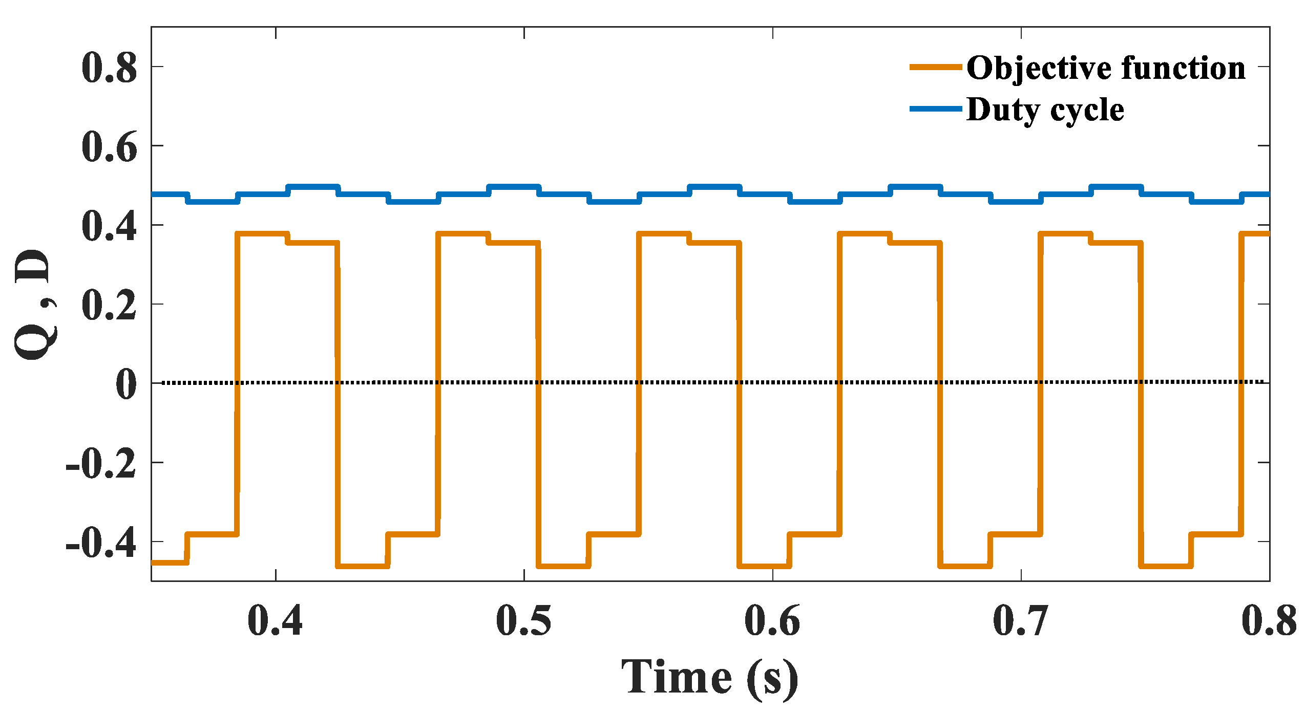
  • Step ③: Calculation of Q using (13).
  • Step ④: Decision of the direction of perturbation of D.
  • Step ⑤: Storage of the actual values of the D and VPV.
  • Step ⑥: Transmitting the updated D to the converter.
The last five steps keep executing periodically after a predefined sampling time, denoted by TS.
Stateflow is a powerful tool for model-based controller design using a finite state. It contains tools making the development and debugging processes easy and fast, such as access to the values of variables during the algorithm execution, and the possibility to carry out checks of the errors when executing the algorithm. It provides an efficient C code generation for target hardware [30]. Figure 8 displays the chart of the CSL-based MPPT under the Stateflow environment. The CSL chart is a set of finite states that represent the possible operating modes of the CSL-MPPT algorithm. The execution steps of the CSL method that are depicted in the flowchart of Figure 7 are reproduced in the chart of Figure 8. Thus, the steps of construction of the CSL Stateflow chart are presented in Figure 8, as follows:
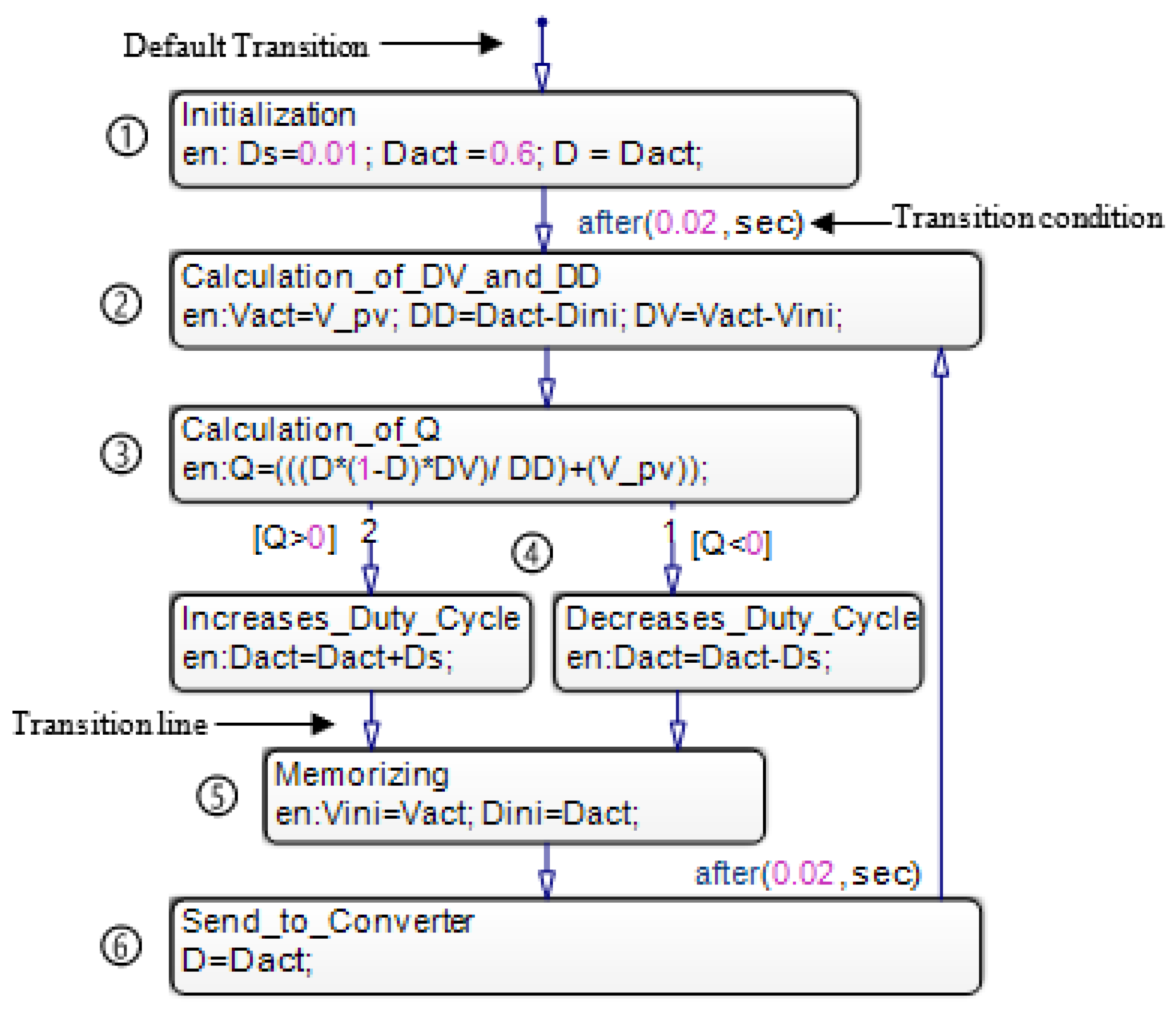
  • The initialization of D and the step-size of the duty cycle perturbation (DS) are made in the first state labeled ①.
  • VPV sensed after TS = 20 ms and ΔV, ΔD, denoted by DV, DD, respectively, can be calculated during state ② activation.
  • In state ③, ΔV, and ΔD values are used to calculate Q.
  • The decision of the perturbation direction of D is made by executing either Increases_Duty_Cycle or Decreases_Duty_Cycle states ④, depending on the sign of Q.
  • In state ⑤, the actual values of VPV and D are stored for the next MPPT cycle.
  • The updated D is transmitted to the converter in state ⑥.

4. Simulation of the Proposed CSL-MPPT Method

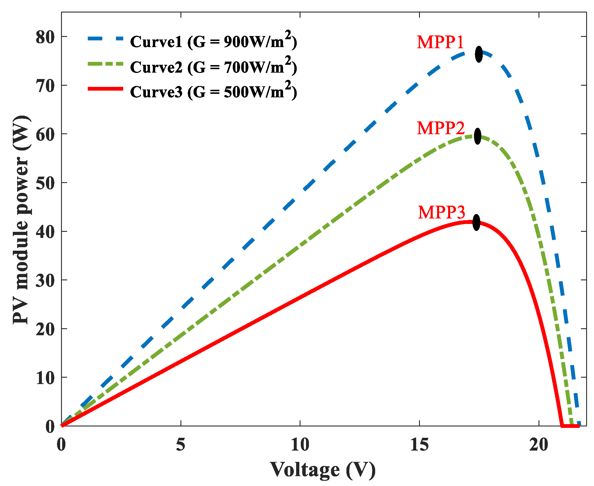
4.1. The Test Environment Used for Simulation

The simulation test of the proposed CSL-MPPT method is carried out under a MATLAB/Simulink/Stateflow environment. The test workbench used for simulation is composed of the one-diode equivalent model of the PV panel, with specifications given in Table 3. The latter is feeding a resistive load (RL) through the buck-boost converter. The buck-boost is constructed to work in a continuous conduction mode (CCM), with the next specifications: L = 4 mH, C1 = 3300 μF, and C2 = 3300 μF, nominal output voltage VO_max = 30 V, the efficiency of buck-boost converter is more than 92%, and the switching frequency ( f s ) is equal to 20 kHz.
MPPT algorithms for PV systems are usually tested under the EN 50,530 dynamic efficiency test [31], where the sharpest irradiance slope is 100 W/m2/s (per second). Nevertheless, due to the expansion of PV technology utilization in different projects such as car-mounted PV, and backpack PV, PV modules can be exposed to fast irradiance disturbance, i.e., up to 100 W/m2/ms (per millisecond) [32]. Consequently, MPPT behavior is examined under a very sharp irradiance variation, i.e., step waveform. The test profile used in the simulation is composed of three P-V curves applied successively in a time interval of 2 s. These three P-V curves are shown in Figure 9. The curves 1, 2, and 3 are obtained by subjecting the PV panel to 900 W/m2, 700 W/m2, and 500 W/m2, with MPP1 (17.36 V, 76.90 W), MPP2 (17.29 V, 59.50 W), and MPP3 (17.11 V, 41.90 W), and applied on the following time intervals in the test profile (0 s, 0.8 s), (0.8 s, 1.4 s), and (1.4 s, 2 s), respectively. The temperature is kept unchanged at 25 °C throughout the testing period. In the proposed method, the MPPT sampling time TS is 20 ms and the step-size of the duty cycle perturbation is 1%, i.e., DS = 0.01.

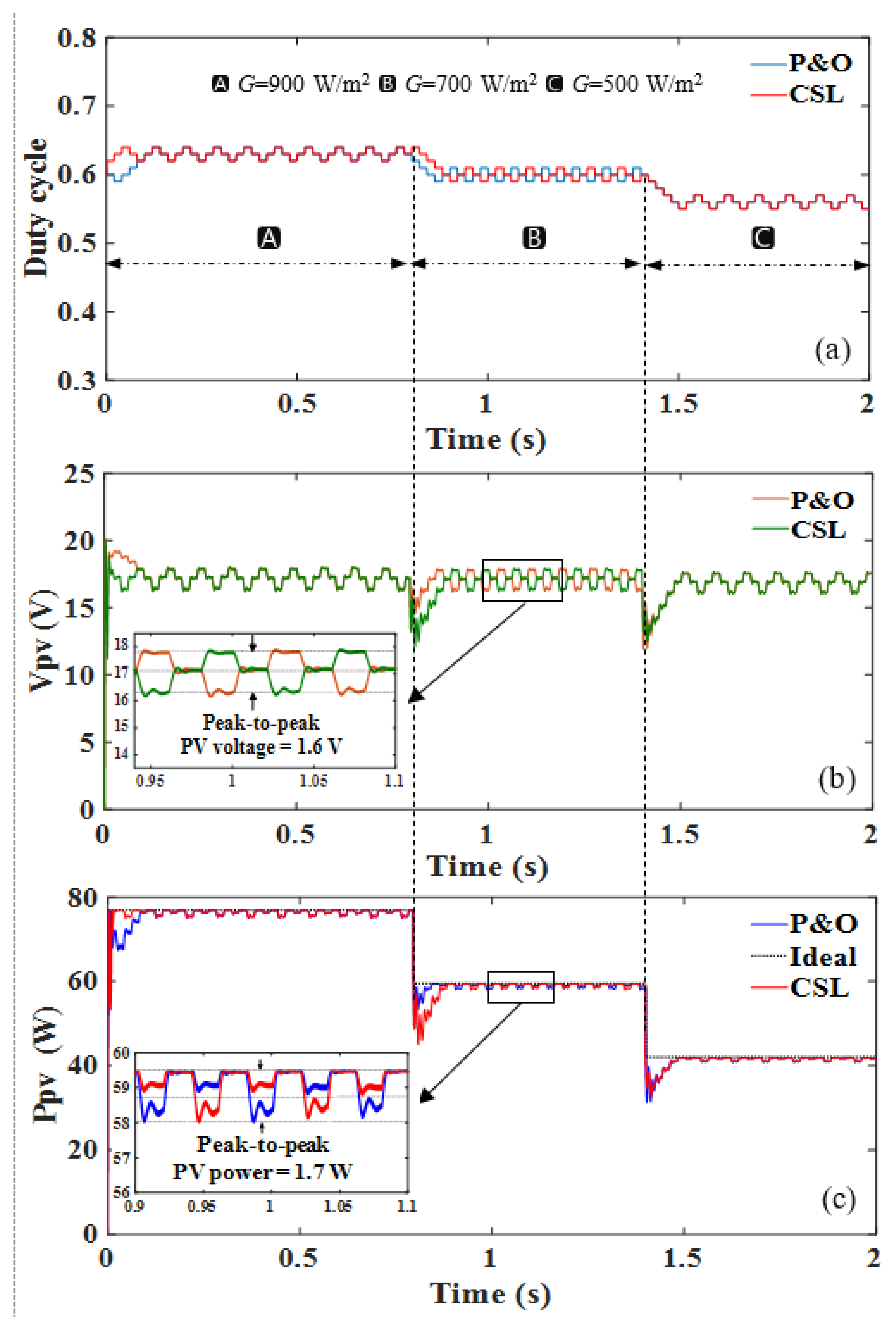
4.2. Results and Discussion

The performance of the CSL-MPPT algorithm is compared with conventional P&O. Both MPPTs are examined under the test profile of the three P-V curves mentioned earlier. For both algorithms, the waveforms of D, VPV, and PPV, are shown in Figure 10a–c, respectively. At the beginning, MPP1 is tracked by both algorithms in less than 100 ms with a similar tracking speed. MPP2 is tracked also within 80 ms, but this time, CSL is a bit slower in tracking. The tracking of MPP3 has been successfully made by both algorithms with the same tracking speed. Consequently, both algorithms show an almost similar tracking speed. In addition, the tracking efficiencies under this test profile are found to be equal to 98.82% for both algorithms. Hence, it can be concluded that the proposed CSL-MPPT has an almost identical performance with the P&O.
Figure 11 shows a zoomed portion of the steady-state oscillation around the MPP using the CSL algorithm. The power versus time is shown in Figure 11a where the peak-to-peak power oscillation is confined within 1.7 W. The three-level operation of D is shown in Figure 11b, where D oscillates around the optimal duty cycle value (Dopt) between three points: A = Dopt DS, B = Dopt, and C = Dopt + DS. Figure 11c shows the duty cycle variation with respect to time.
The variation of Q is shown in Figure 12. When the MPP is tracked, Q oscillates around zero during the steady-state regime, then it is pulled away from the zero during the search for the new MPP (for MPP2 at 0.8 s, and MPP3 at 1.4 s).
A zoomed portion of the variation of Q together with D at the steady-state regime is shown in Figure 13, where the dynamic behavior of the model is considered in the simulation. As it can be seen in Figure 13, the oscillation of Q is irregular due to the inherent ripple of the pseudo-periodic step responses of the input capacitor voltage when the duty cycle is perturbed by the MPPT. Although Q can be easily influenced by this ripple, the tracking capability will not be influenced as long as the duty cycle step-size is chosen to be large enough to guarantee the correct measurement of the sign of Q. On the other hand, Figure 14 shows the variation of Q in the ideal case without considering the noise and the ripple of the input capacitor, i.e., the operation in the Q-D characteristics directly reached the final value. It can be seen that Q is oscillating around fixed points during the steady state.
For the load disturbance, the tracking performance of the CSL-MPPT algorithm is examined under the variation of the load, where a step-change in load is introduced at t = 0.8 s from 10 to 5 Ω. Then, it is stepped up to 10 Ω again at t = 1.4 s. The waveforms of D, VPV, and PPV, are shown in Figure 15a–c, respectively. At the beginning, the MPP1 is tracked in less than 60 ms by the proposed CSL-MPPT. Then, the MPP2 and MPPT3 are tracked within 180 ms. Consequently, the power is rapidly restored after a brief dip when the load change takes place. It can be concluded that the tracking performance of the proposed CSL-MPPT is able to track the MPP under load disturbance effectively.
For more clarification, Figure 16 shows a zoomed portion of the tracking performance of CSL-MPPT of the PV-buck-boost converter system under variation of the load from 5 Ω to 10 Ω with fixed irradiance at 900 W/m2. It can be seen that power versus time is shown in Figure 16a, where the perturbation steps of the tracking to the new MPP are illustrated in Figure 16b. The increments of the duty cycle operation are shown in Figure 16c, where the algorithm needs seven successive increments of the duty cycle to reach the new MPP. Furthermore, the objective function versus time is shown in Figure 16d, where the perturbation steps to annul the objective function, which corresponds to tracking the new MPP, are illustrated in Figure 16e.

5. Hardware Validation

5.1. Experimental Set-Up

The efficiency of the suggested CSL-MPPT is verified experimentally using the hardware test bench shown in Figure 17. The latter is composed of an Agilent PV array simulator (E4360A Modular SAS) used to emulate the electrical behavior of PV modules/arrays using dc voltage controlled-current source. The simulator is feeding a variable-resistive load through a low power buck-boost converter (100 W) and the nominal output voltage VO_max = 30 V with the following specifications: L = 4 mH, C1 = 3300 μF, and C2 = 3300 μF, working under a switching frequency of fs = 20 kHz. The LEM LV-25P hall-effect sensor is utilized to sense the PV module voltage and transmit the calibrated feedback signal (within the range 0 V–3.3 V) to the Arduino DUE board. Furthermore, the gate-drive circuit based on the HCPL3120 IC driver and an isolated power supply are used to control the MOSFET power switch.
The Arduino DUE board is utilized as a target hardware for the CSL-MPPT controller developed under a MATLAB/Simulink/Stateflow environment. The support package of Matlab/Simulink for Arduino is utilized to transform the CSL controller into an Arduino-compatible C code, which is, again, compiled and loaded to the SAM3X8E microcontroller of the Arduino DUE. Figure 18 shows the model-based CSL controller compiled and loaded to the Arduino DUE using the Simulink support package for Arduino hardware [33]. During the real-time operation, the numerical voltage value is transmitted to the CSL Stateflow chart (Explained earlier in Section 3.3) through a dedicated read block for Arduino hardware, wherein the input pin (ADC channel) of the sensed signal can be assigned.
The PWM module of the SAM3X8E microcontroller integrates eight separate channels, each one can generate two complementary outputs [34]. The characteristics of the output waveforms such as frequency, duty cycle, and polarity can be configured through the dedicated control registers using the assembly code. For this purpose, the S-function builder block is used to configure the PWM module and to generate the PWM signal according to the computed duty cycle value by the CSL Stateflow chart. The assembly code implemented through the S-function is shown in Figure 19. The PWM module configuration can be summarized in the following steps:
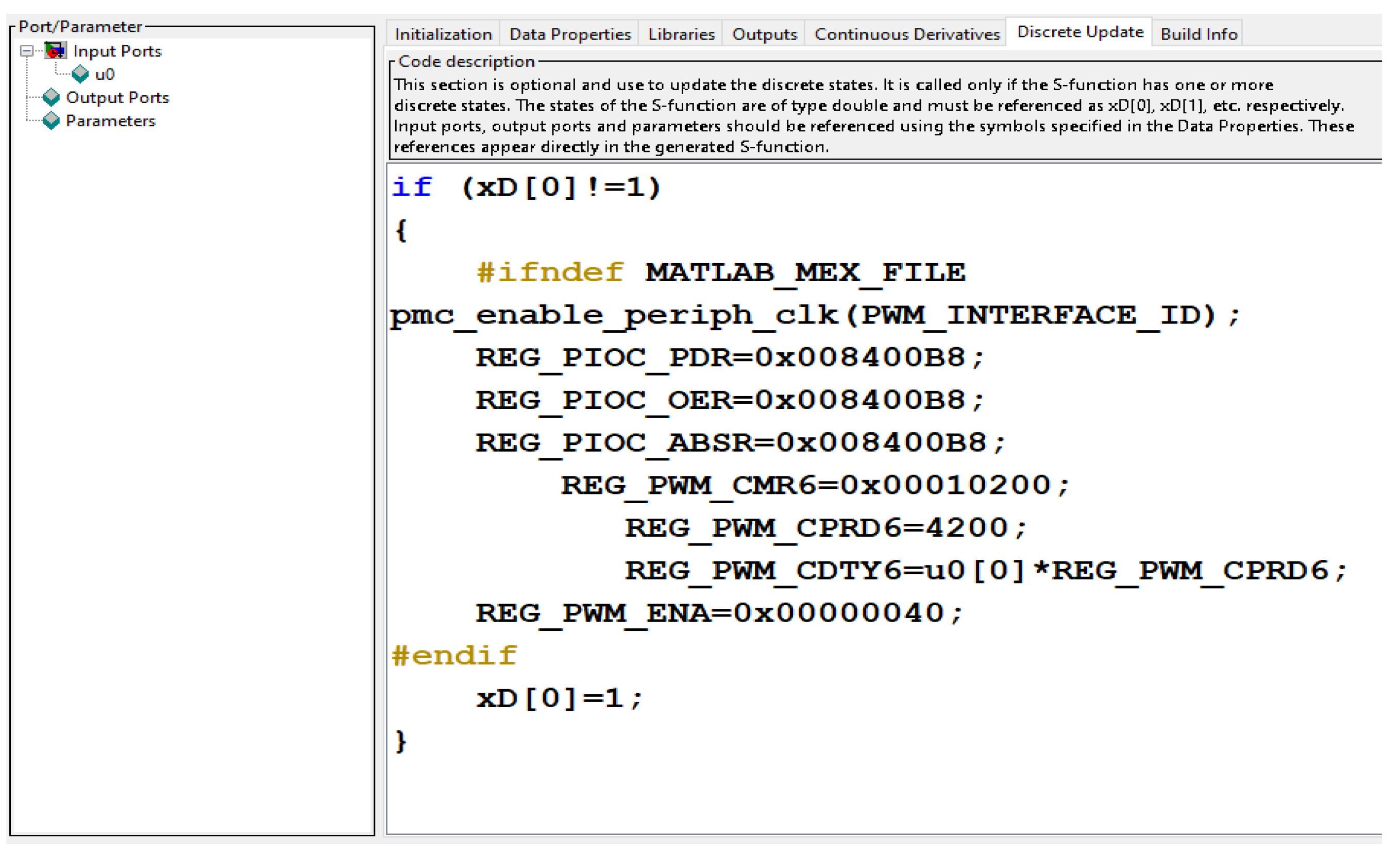
  • Multiplexing the parallel input/output of port C (PIOC) with PWM channel 6 output: The register REG_PIOC_PDR is used to disable PIOC; then, the REG_PIOC_ABSR register is used to assign the PIOC to peripheral A or B; after that, the PIOC is enabled again by using REG_PIOC_OER.
  • Switching the frequency configuration: the channel mode register REG_PWM_CMR6 is used to set the required clock of channel 6 and the characteristics of the output waveforms. Then, the value of REG_PWM_CPRD6 is calculated such that the required frequency can be accurately generated, i.e., to get a 20 kHz-switching frequency, since the master clock (84 MHz) is selected, the value of REG_PWM_CPRD6 is obtained as follows: 84 MHz/20 KHz = 4200.
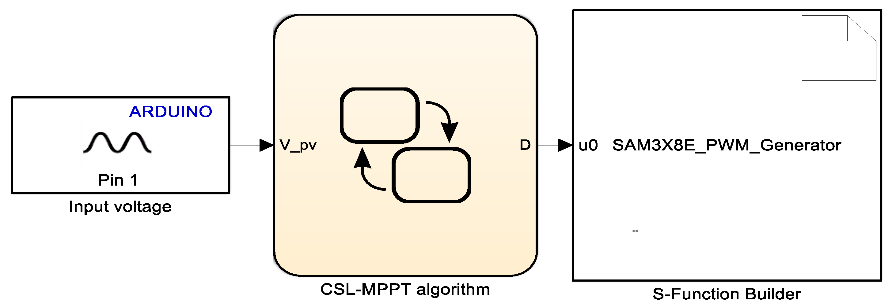
  • Updating the duty cycle value: the updating value of the duty cycle is configured through the REG_PWM_CDTY6 register as follows: REG_PWM_CDTY6 = u0[0] × REG_PWM_CPRD6, where u0[0] contains the computed duty cycle value obtained from the Stateflow of the CSL-MPPT algorithm [34].

5.2. Experimental Results and Discussion

The CSL-MPPT and P&O-MPPT methods are experimentally evaluated under the same operating condition with TS = 200 ms, and DS = 0.02. The tracking process is re-initialized every 15 min to avoid fault occurrence and software errors. Further, the tracking capability of the proposed CSL algorithm is proven under variable irradiance changes and load disturbance.

5.2.1. Experimental Validation under the Irradiance Change Test:

The transient state of the test profile is initialized, and the irradiance is at 900 W/m2, then stepped to 700 W/m2 at t = 7 s and stepped to 500 W/m2 at t = 14 s; the results are shown in Figure 20. The voltage, current, and power oscillograms for both CSL and P&O algorithms are shown in Figure 20a,b, respectively. In addition, a zoomed portion of the steady-state oscillation of voltage, current, and power of the CSL algorithm is shown in Figure 20c. Regarding the tracking speed, both CSL and P&O can track MPP in less than 750 ms. Similar to the simulation finding, both algorithms have an almost similar performance.
Table 4 presents a comparison between the proposed CSL and conventional P&O algorithms from all aspects. From this table, it can be seen that both CSL and P&O have a similar tracking performance. The CSL outperforms the P&O in terms of computational requirements, as shown in Figure 21, where the computational burden and the sensor cost of implementation are decreased by 24.3%, and 27.95%, respectively. As can be seen in Table 4, the computation time required by the P&O is higher than that required by the CSL algorithm. This is because the P&O needs two ADC for the current and voltage signal conversions, while the proposed CSL uses only one ADC for the voltage signal conversion.

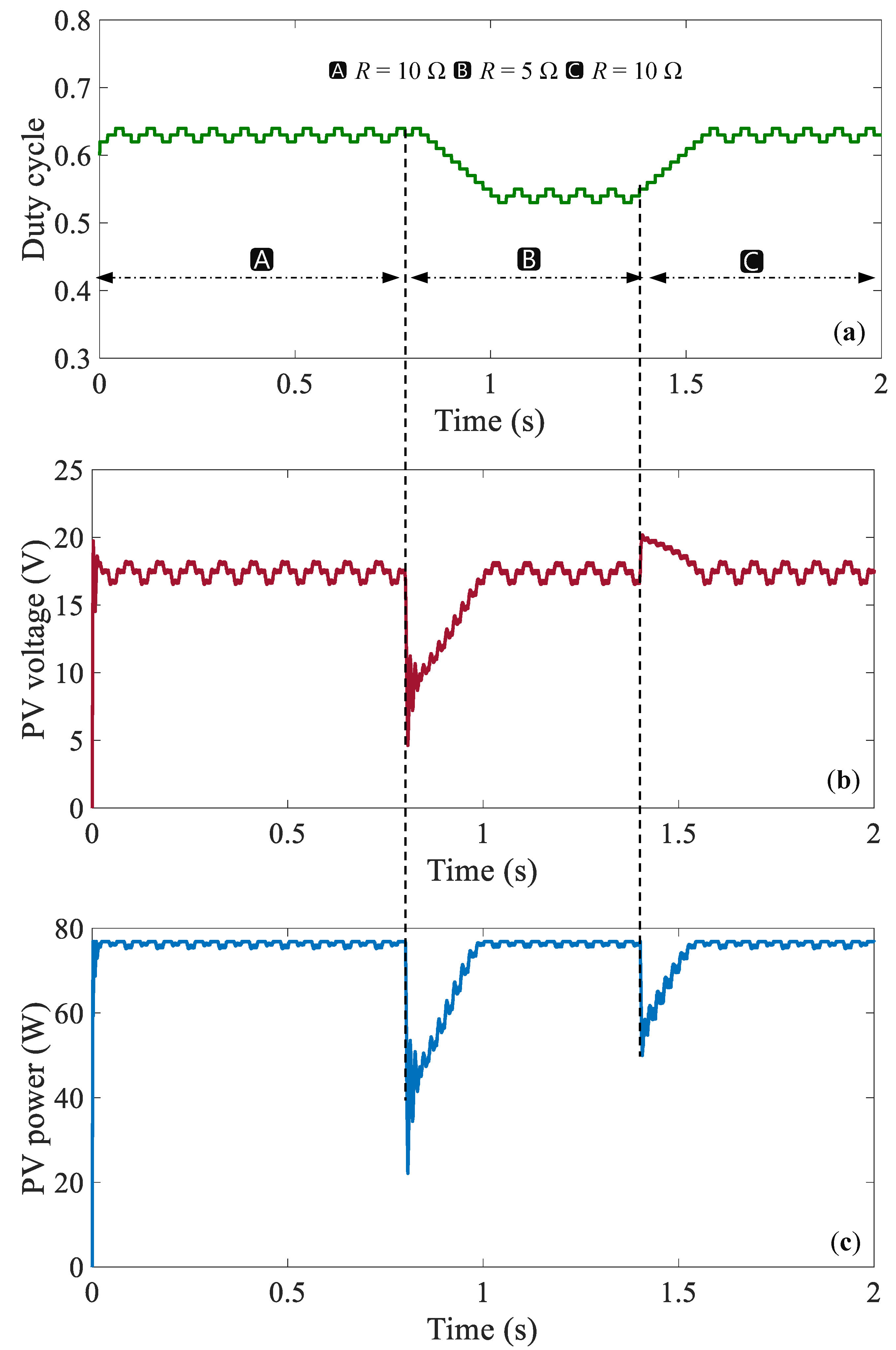
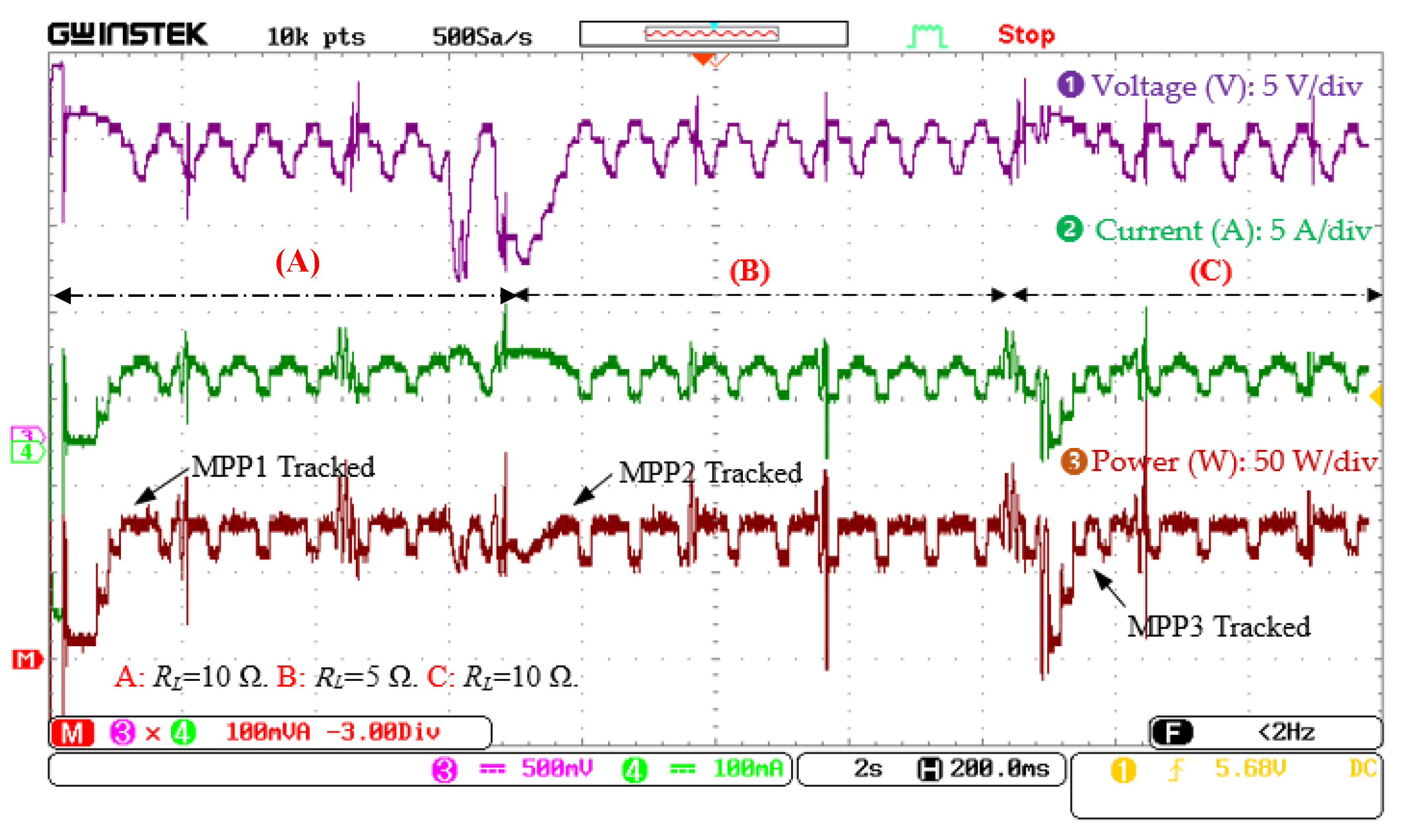
5.2.2. Experimental Validation in Presence of Load Disturbances

To examine the influence of the load changes on the performance of the proposed CSL-MPPT, a step-change in load for CSL-MPPT is introduced at t = 7 s from 10 to 5 Ω. Then, it is stepped up to 10 Ω again at t = 15 s. The experimental results of the waveforms are displayed in Figure 22. As can be observed from these waveforms, the effect of the load change on the tracking performance of the CSL-MPPT is almost negligible; the power is rapidly restored after a brief dip when the load change takes place.

6. Conclusions

This paper presents a current sensorless maximum power point tracking algorithm for PV systems implemented using the Arduino DUE microcontroller. The proposed method is dependent on the buck-boost converter, where a predefined objective function derived from its mathematical model is used for its implementation. A comparative evaluation of the proposed method and conventional P&O algorithm has been carried out under a Matlab/Simulink/Stateflow environment. Additionally, an experimental test has been carried out to validate the simulation where the Simulink support package for Arduino hardware was used to generate the code for the microcontroller. The reduction percentage of the total cost and the computation burden were 27.95% and 24.3%, respectively. The proposed current sensorless scheme could be extended to deal with partial shading conditions.

Author Contributions

Data curation, N.O.; Formal analysis, N.O.; Investigation, N.O.; Methodology, L.A.; Resources, A.A.; Supervision, S.M.; Writing—original draft, N.O.; Writing—review & editing, M.K., B.B. and S.M. All authors have read and agreed to the published version of the manuscript.

Funding

This work is supported by the Universiti Tenaga Nasional grant no. IC6-BOLDREFRESH2025 (HCR) under the BOLD2025 Program.

Conflicts of Interest

The authors declare no conflict of interest.

References

  1. Achour, L.; Bouharkat, M.; Assas, O.; Behar, O. Hybrid model for estimating monthly global solar radiation for the Southern of Algeria:(Case study: Tamanrasset, Algeria). Energy 2017, 135, 526–539. [Google Scholar] [CrossRef]
  2. Kok Soon, T.; Mekhilef, S.; Safari, A. Simple and low cost incremental conductance maximum power point tracking using buck-boost converter. J. Renew. Sustain. Energy 2013, 5, 023106. [Google Scholar] [CrossRef]
  3. Azevedo, G.; Cavalcanti, M.; Oliveira, K.; Neves, F.; Lins, Z. Comparative evaluation of maximum power point tracking methods for photovoltaic systems. J. Sol. Energy Eng. 2009, 131, 031006. [Google Scholar] [CrossRef]
  4. Kjær, S.B. Evaluation of the “hill climbing” and the “incremental conductance” maximum power point trackers for photovoltaic power systems. IEEE Trans. Energy Convers. 2012, 27, 922–929. [Google Scholar] [CrossRef]
  5. Karami, N.; Moubayed, N.; Outbib, R. General review and classification of different MPPT Techniques. Renew. Sustain. Energy Rev. 2017, 68, 1–18. [Google Scholar] [CrossRef]
  6. Ahmed, J.; Salam, Z. An enhanced adaptive P&O MPPT for fast and efficient tracking under varying environmental conditions. IEEE Trans. Sustain. Energy 2018, 9, 1487–1496. [Google Scholar]
  7. Safari, A.; Mekhilef, S. Simulation and hardware implementation of incremental conductance MPPT with direct control method using cuk converter. IEEE Trans. Ind. Electron. 2010, 58, 1154–1161. [Google Scholar] [CrossRef]
  8. Huynh, D.C.; Dunnigan, M.W. Development and comparison of an improved incremental conductance algorithm for tracking the MPP of a solar PV panel. IEEE Trans. Sustain. Energy 2016, 7, 1421–1429. [Google Scholar] [CrossRef]
  9. Lashab, A.; Sera, D.; Guerrero, J.M. A dual-discrete model predictive control-based MPPT for PV systems. IEEE Trans. Power Electron. 2019, 34, 9686–9697. [Google Scholar] [CrossRef] [Green Version]
  10. Valenciaga, F.; Inthamoussou, F. A novel PV-MPPT method based on a second order sliding mode gradient observer. Energy Convers. Manag. 2018, 176, 422–430. [Google Scholar] [CrossRef]
  11. Bawa, D.; Patil, C. Fuzzy control based solar tracker using Arduino Uno. Int. J. Eng. Innov. Technol. 2013, 2, 179–187. [Google Scholar]
  12. Kermadi, M.; Berkouk, E.M. Artificial intelligence-based maximum power point tracking controllers for Photovoltaic systems: Comparative study. Renew. Sustain. Energy Rev. 2017, 69, 369–386. [Google Scholar] [CrossRef]
  13. Labbi, Y.; Attous, D.B. Maximum Photovoltaic Power Tracking under Different Conditions Using a Genetic Algorithm and Particle Swarm Optimization. J. Electr. Control Eng. Dec 2012, 2, 7–13. [Google Scholar]
  14. Ram, J.P.; Rajasekar, N. A novel flower pollination based global maximum power point method for solar maximum power point tracking. IEEE Trans. Power Electron. 2016, 32, 8486–8499. [Google Scholar]
  15. Du, Y.; Yan, K.; Ren, Z.; Xiao, W. Designing localized MPPT for PV systems using fuzzy-weighted extreme learning machine. Energies 2018, 11, 2615. [Google Scholar] [CrossRef] [Green Version]
  16. Pillai, D.S.; Ram, J.P.; Ghias, A.M.; Mahmud, M.A.; Rajasekar, N. An Accurate, Shade Detection-Based Hybrid Maximum Power Point Tracking Approach for PV Systems. IEEE Trans. Power Electron. 2019, 35, 6594–6608. [Google Scholar] [CrossRef]
  17. Fannakh, M.; Elhafyani, M.L.; Zouggar, S. Hardware implementation of the fuzzy logic MPPT in an Arduino card using a Simulink support package for PV application. IET Renew. Power Gener. 2018, 13, 510–518. [Google Scholar] [CrossRef]
  18. Killi, M.; Samanta, S. An adaptive voltage-sensor-based MPPT for photovoltaic systems with SEPIC converter including steady-state and drift analysis. IEEE Trans. Ind. Electron. 2015, 62, 7609–7619. [Google Scholar] [CrossRef]
  19. Motahhir, S.; Chalh, A.; El Ghzizal, A.; Derouich, A. Development of a low-cost PV system using an improved INC algorithm and a PV panel Proteus model. J. Clean. Prod. 2018, 204, 355–365. [Google Scholar] [CrossRef]
  20. Killi, M.; Samanta, S. Voltage-Sensor-Based MPPT for Stand-Alone PV Systems Through Voltage Reference Control. IEEE J. Emerg. Sel. Top. Power Electron. 2018, 7, 1399–1407. [Google Scholar] [CrossRef]
  21. Dasgupta, N.; Pandey, A.; Mukerjee, A.K. Voltage-sensing-based photovoltaic MPPT with improved tracking and drift avoidance capabilities. Sol. Energy Mater. Sol. Cells 2008, 92, 1552–1558. [Google Scholar] [CrossRef]
  22. Metry, M.; Shadmand, M.B.; Balog, R.S.; Abu-Rub, H. MPPT of photovoltaic systems using sensorless current-based model predictive control. IEEE Trans. Ind. Appl. 2016, 53, 1157–1167. [Google Scholar] [CrossRef]
  23. Veerachary, M.; Senjyu, T.; Uezato, K. Voltage-based maximum power point tracking control of PV system. IEEE Trans. Aerosp. Electron. Syst. 2002, 38, 262–270. [Google Scholar] [CrossRef] [Green Version]
  24. Harrag, A.; Messalti, S.; Daili, Y. Innovative Single Sensor Neural Network PV MPPT. In Proceedings of the 2019 6th International Conference on Control, Decision and Information Technologies (CoDIT), Paris, France, 23–26 April 2019; pp. 1895–1899. [Google Scholar]
  25. Kermadi, M.; Mekhilef, S.; Salam, Z.; Ahmed, J.; Berkouk, E.M. Assessment of maximum power point trackers performance using direct and indirect control methods. Int. Trans. Electr. Energy Syst. 2020, 30, e12565. [Google Scholar] [CrossRef]
  26. Ishaque, K.; Salam, Z.; Shamsudin, A.; Amjad, M. A direct control based maximum power point tracking method for photovoltaic system under partial shading conditions using particle swarm optimization algorithm. Appl. Energy 2012, 99, 414–422. [Google Scholar] [CrossRef]
  27. Kermadi, M.; Salam, Z.; Ahmed, J.; Berkouk, E.M. An effective hybrid maximum power point tracker of photovoltaic arrays for complex partial shading conditions. IEEE Trans. Ind. Electron. 2018, 66, 6990–7000. [Google Scholar] [CrossRef]
  28. Loukriz, A.; Haddadi, M.; Messalti, S. Simulation and experimental design of a new advanced variable step size Incremental Conductance MPPT algorithm for PV systems. ISA Trans. 2016, 62, 30–38. [Google Scholar] [CrossRef] [PubMed]
  29. Slotine, J.-J.E.; Li, W. Applied Nonlinear Control; Prentice Hall: Englewood Cliffs, NJ, USA, 1991; Volume 199. [Google Scholar]
  30. Kermadi, M.; Salam, Z.; Berkouk, E.M. A rule-based power management controller using stateflow for grid-connected PV-battery energy system supplying household load. In Proceedings of the 2018 9th IEEE International Symposium on Power Electronics for Distributed Generation Systems (PEDG), Charlotte, NC, USA, 25–28 June 2018; pp. 1–6. [Google Scholar]
  31. Bründlinger, R.; Henze, N.; Häberlin, H.; Burger, B.; Bergmann, A.; Baumgartner, F. prEN 50530–The New European Standard for Performance Characterisation of PV Inverters. In Proceedings of the 24th European Photovoltaic Solar Energy Conference, Hamburg, Germany, 21–24 September 2009; pp. 3105–3109. [Google Scholar]
  32. Zurbriggen, I.G.; Ordonez, M. PV Energy Harvesting Under Extremely Fast Changing Irradiance: State-Plane Direct MPPT. IEEE Trans. Ind. Electron. 2019, 66, 1852–1861. [Google Scholar] [CrossRef]
  33. Simulink Support Package for Arduino Hardware. 2020. Available online: https://www.mathworks.com/matlabcentral/fileexchange/40312-simulink-support-package-for-arduino-hardware (accessed on 7 September 2022).
  34. Atmel. SAM3X/SAM3A Series Datasheet; Atmel Corporation: San Jose, CA, USA, 2015; p. 1459. [Google Scholar]
  35. Voltage Transducer LV25P. 2020. Available online: https://www.lem.com/sites/default/files/products_datasheets/lv_25-p.pdf (accessed on 3 October 2022).
  36. Current Transducer LA25-NP/SP25. 2020. Available online: https://www.lem.com/sites/default/files/products_datasheets/la%2025-np%20sp25.pdf (accessed on 3 October 2022).
Figure 1. The topology for the PV system under study and its associated MPPT control unit.
Energies 15 07811 g001
Figure 2. Equivalent circuit of one diode model of the PV cell.
Energies 15 07811 g002
Figure 3. The variation of P and P with respect to D.
Energies 15 07811 g003
Figure 4. Operation of the MPP on the P-D, Q-D, and V-D characteristics for the buck-boost converter.
Energies 15 07811 g004
Figure 5. Electrical characteristics of the PV-buck-boost converter under variation of the load with fixed irradiance at 900 W/m2 (a) P-D characteristics, (b) Q-V characteristics, and (c) V-D characteristics.
Energies 15 07811 g005
Figure 6. The control diagram of the proposed CSL-MPPT control.
Energies 15 07811 g006
Figure 7. Flowchart of the proposed CSL-MPPT method.
Energies 15 07811 g007
Figure 8. The Stateflow chart of the proposed CSL algorithm.
Energies 15 07811 g008
Figure 9. P-V characteristics of the test profile.
Energies 15 07811 g009
Figure 10. The simulation result of the tracking waveforms for both P&O-MPPT and CSL-MPPT algorithms: (a) duty cycle, (b) PV module voltage, and (c) PV module power.
Energies 15 07811 g010
Figure 11. Steady-state oscillation around the MPP using the CSL algorithm with the three-level operation: (a) power versus time, (b) PV power versus duty cycle, and (c) duty cycle versus time.
Energies 15 07811 g011
Figure 12. Oscillation of Q around zero during MPP tracking.
Energies 15 07811 g012
Figure 13. Zoomed portion of Q oscillation considering the dynamics of the system.
Energies 15 07811 g013
Figure 14. Zoomed portion of the oscillation of Q using the ideal model.
Energies 15 07811 g014
Figure 15. The simulation result of the tracking waveforms for the proposed CSL-MPPT under load disturbance from 10 Ω to 5 Ω, then from 5 Ω to 10 Ω with fixed irradiance at 900 W/m2: (a) duty cycle versus time, (b) PV module voltage versus time, and (c) PV module power versus time.
Energies 15 07811 g015
Figure 16. The tracking performance of CSL-MPPT of the PV-buck-boost converter system under variation of the load from 5 Ω to 10 Ω with fixed irradiance at 900 W/m2: (a) power versus time, (b) PV power versus duty cycle, and (c) duty cycle versus time, (d) objective function versus time, and (e) objective function versus duty cycle.
Energies 15 07811 g016
Figure 17. The hardware set-up used for the experimental verification.
Energies 15 07811 g017
Figure 18. The Simulink model of the CSL controller loaded to the target hardware.
Energies 15 07811 g018
Figure 19. The utilization of the S-function builder to configure the PWM module using the assembly code.
Energies 15 07811 g019
Figure 20. The tracking performance under irradiance changes: (a) experimental waveforms of CSL-MPPT, (b) experimental waveforms of the P&O-MPPT, and (c) the zoom portion of the three-level operation of the CSL-MPPT.
Energies 15 07811 g020
Figure 21. Comparison of the computation time required by the CSL and P&O algorithms.
Energies 15 07811 g021
Figure 22. Experimental waveforms of the CSL-MPPT in the presence of the load disturbances.
Energies 15 07811 g022
Table 1. MPPT algorithms experimentally validated using the Arduino platform.
AuthorsMPPT AlgorithmMicrocontroller Used
Killi et al., 2015 [18]Voltage-based MPPTAtmega2560
Fannakh et al., 2018 [17]Fuzzy logicAtmega2560
Motahir et al., 2018 [19]Modified Incremental Conductance (IncCond)Atmega328p
Killi et al., 2018 [20]Voltage-Reference-based MPPTAtmega2560
Table 2. Review of different published current sensorless MPPT techniques.
AuthorsObjective Function (Q)ConverterController Type
Killi et al. [18] D ( 1 D ) d V P V + V P V d D SEPICAtmega2560
(AVR core)
Dasgupta et al. [21] V P V d D + D d V P V BuckADuC831 (8052 core)
Harrag et al. [24]ANN based on
d V P V = ( d D V P V ) / ( 1 D )
BoostMatlab/
Simulink
Proposed V P V + D 1 D d V P V / d D Buck-boostSAM3X8E (ARM-Cortex M3 core)
Table 3. Characteristics of the DM-85 PV panel at standard test conditions (STC).
ParametersLabelsValues
Max PowerPmax85 W
Max VoltageVmax17.85 V
Max currentImax4.77 A
Short-CircuitIsc5.15 A
Open Circuit voltageVoc21.8 V
Temperature coefficient of ISCKV0.06%/°C
Temperature coefficient of VOCKI−0.35%/°C
Number of cellsNS36
Table 4. Performance comparison between the proposed CSL and conventional P&O algorithm.
AlgorithmRipple in PowerConvergence TimeEfficiencyComputation TimeSensors [35,36]
(Cost)
P&O7.5 W750 ms98.4%37 μsVoltage and current
(104.27 $)
CSL7.5 W750 ms98.4%28 μsVoltage
(75.13 $)
Publisher’s Note: MDPI stays neutral with regard to jurisdictional claims in published maps and institutional affiliations.

