LCOE-Based Optimization for the Design of Small Run-of-River Hydropower Plants

Abstract

Run-of-river hydropower plants are a cost-efficient technology that produce a power output proportional to the instantaneous flow of water diverted from the exploited stream by exploiting several mechanical, hydraulic, and electric devices. However, as no storage is available, its design and operation is tailored according to the unpredictability of its power generation. Hence, the modelling of this type of power plants is a necessity for the promotion of its development. Accordingly, based on models from the literature, this study proposes a comprehensive methodology for optimally designed small run-of-river hydropower plants based on a levelized cost of energy (LCOE). The proposed methodology aims at facilitating a faster design for more cost-effective and energy-efficient small hydropower plants. Depending on the average daily flow rates and the gross head of a given site, the model proposed in this study calculates the diameter, thickness, and length of a penstock; it also suggests the optimal selection of a turbine, determines the admissible suction head of a turbine for its optimal implementation, and determines the optimal number of turbines, all in order to minimize the LCOE of the proposed project. The model is tested to design a small run-of-river hydropower plant with a capacity of 6.32 MW exploiting the river Nyong in Mbalmayo. The results confirm the profitability of the investment with an LCOE of around 0.05 USD/kWh, which is the lowest limit value of the LCOE range for small hydropower plants, as presented in the IPCC (Intergovernmental Panel on Climate Change) report, assuming a project lifespan of 50 years and a discount rate of 12.5%. These results also show that it may be worth to provide the energy sector with a small hydropower design tool with a graphical interface. In addition, it would be appropriate to use a similar method in an off-grid context where a hydropower plant, with or without storage, is combined with another source to meet the electrical needs of a given population.

1. Introduction

As of today, around 81.4% of the primary energy exploited in the world is of fossil origin, mainly in the form of coal, oil, and natural gas [1]. This shows that fossil fuels still continue to play a dominant role in the energy sector, despite the drawbacks on the environment and ecosystems that accompany their exploitation.

Thus, this challenge of reducing the consumption of fossil fuels, combined with the need for increasing energy production capacity to meet the expected increase in the global energy demand, forces the international community to increase the contribution of renewable energies to world energy production.

Of all the renewable energy sources, hydropower is thus far among the most efficient and reliable resources because it has a simple but very mature technology [2,3].

However, when it comes to hydropower, small run-of-river hydropower plants—which is a type of hydropower plant that does not need a reservoir and that, therefore, has its power production instantaneously proportional to the exploited water course—seem more attractive [4].

Indeed, small run-of-river hydropower plants have lower investment costs, less of a harmful impact on the environment, and a shorter construction time when compared to hydroelectric power plant projects with storage [5]. More concretely, they pose fewer problems of inundation and sedimentation, they have less of a harmful impact on fish migration, and they decrease issues regarding navigation on the rivers—which occur in large-scale hydropower projects [6]. Another advantage of run-of-river hydropower projects is the fact that they drive generators with small turbines that can be manufactured locally, thus promoting job creation and economic development through local industry [7]. Due to these advantages, it is also easier to gain public and government acceptance for run-of-river hydropower projects compared to hydropower projects with storage that require large areas of submersion [6].

In the work of Alexandros et al. [8], it was found that the potential of small hydropower (1–10 MW in this context) in Sub-Saharan Africa is estimated at 21,800 MW and run-of-river hydropower plants are generally categorized as small hydropower plants [9,10,11,12,13]. Additionally, more particularly in Cameroon, the small hydropower capacity is estimated at 970 MW, according to the UNIDO small hydropower development report [14]. Small hydropower and hence run-of-river systems can be an appropriate option for rural electrification in Africa.

Despite the fact that run-of-river hydroelectric plants represent a better alternative to installations with dams [15], their unforeseeable power production can make their design and exploitation very complex, especially when they have no pondage, without an accurate estimation of their energy production over the lifetime of the project.

This study aims to develop a model for the sizing and techno-economical optimization of small run-of-river hydropower plants, which could help designers, hydropower engineers, and even decision makers to deal with run-of-river hydropower plants prefeasibility studies in a more efficient, easier, and faster way. Unlike most of the existing models (such as HOMER, Retscreen), which are unusable without a minimum of data, the model presented in this article relies on a minimum of data (daily average flows and gross head) in order to provide a maximum of results. Existing models sometimes require special knowledge in the field of energy, pre-sizing in the first step or a good knowledge of the market for hydroelectric equipment (e.g., the price of the equipment, cost of maintenance and exploitation, etc.).

The study presented in this paper begins by identifying and analyzing existing models used in the literature for hydropower plant projects (such as models for the sizing of plant components and for estimating energy production—as well as for estimating investment, operation, and maintenance costs). Then, the models that fit the context of our study are selected or adapted and finally, a program is realized using the equations of the selected models and relying on a genetic algorithm for the optimization process. In fact, once the technical model has been developed, it is integrated into an economical model with LCOE as the objective function. The function obtained being a non-differential function because of the discontinuous equations, which are integrated therein, therefore the optimization was made from a genetic algorithm, since today it has been already proven for similar optimization cases [16,17,18].

There are several works relating to the optimal design of hydropower plants, and particularly, small run-of-river hydropower plants, in order to reduce the costs, to maximize energy production, or to maximize profitability of the project [9,15,19,20,21,22,23,24,25,26,27,28,29,30,31,32,33,34,35,36,37,38,39].

Some researchers have focused on the optimal design of the penstock in order to reduce operation and the initial purchase cost since the penstock has a high share in the total small hydropower plant budget [23,24].

Other researchers worked on the choice of the optimal turbine in order to maximize the energy production or the economic benefits of the investment [25,26,27,28,29]. Most of these studies focused on the choice for the optimum nominal flow of a turbine [25,26,27]. Indeed, the nominal flow must be chosen carefully in order to create a hydro project that is profitable and efficient enough.

Many other authors also worked on the development of correlations to estimate the cost of small hydropower plant projects and, therefore, providing tools for the development of models, thereby allowing the techno-economic design optimization of small hydropower plants [30,31,32,33,34,35,36,37].

There are also more complete methods that have been developed that take into consideration several parameters at the same time [9,13,15,19,20,21,22,38,39].

Najmaii and Movaghar [38] worked on a mathematical model that enables the overall design optimization of run-of-river hydropower plants, and which takes into consideration the discharge design, the penstock diameter, the turbine capacity, the number of units, and the type of turbines for the maximization of the yearly energy and yearly benefits.

Athanassassios et al. [13] developed a program for the preliminary evaluation of the potential of small hydropower plant installations, and they took into account economic life, discount rate, Net Present Value, benefit–cost ratio, Internal Rate of Return, payback period, and generation cost, but without information on the design of the components of the plant.

Anagnostopoulos and Papantonis [19,20] presented a numerical model for the maximization of the Net Present Value using a stochastic evolutionary algorithm for the optimization process and used variables such as the type and size of the two turbines considered as well as the penstock diameter.

Santolin et al. [39] developed a techno-economical method for the capacity sizing of a small hydropower plant, which takes into consideration the turbine type, the turbine dimensions, the annual energy production, the maximum installation height (in order to avoid cavitation inception), the machine cost, the Net Present Value, and the Internal Rate of Return in its analyses; however, this was without an optimization process.

Haddad et al. [9] worked on the optimal design, control, and operation of small run-of-river hydropower plants with the honey bee mating optimization algorithm; this was conducted for the determination of the optimal diameter of the penstock, the optimal number of turbines, the type of turbines, and the optimal scheduling of the operation of the plant for maximization of the annual benefit.

Getachew [21] developed a mathematical model for the determination of the design discharge, the installed capacity, and the number of turbines for the optimal configuration of small run-of-river hydropower plants.

Yildiz [15] produced a numerical model that uses a built-in evolutionary algorithm for the maximization of the Net Present Value by optimizing the penstock diameter (while considering the thickness); the type; design flow and configuration of the two turbines considered; and the specific and rotational speed of the two turbines considered (while considering the suction head to avoid cavitation).

More recently, Mohamed et al. [22] developed an optimal planning and preliminary-design model for the maximization of the annual net benefit of run-of-river hydropower projects. Their model uses a genetic algorithm and allows one to determine intake location; the diameter and the length of the penstock and the type; number; and discharge of the turbines.

However, in most run-of-river hydropower plant optimization studies conducted thus far, no more than two turbines were considered in order to avoid making the project too expensive [15,19,20].

In this study, we review and develop a comprehensive design methodology for multi-turbines that combines mechanical, hydraulic, and electric limitations. The model proposed enables the use of more than two turbines. In fact, although a larger number of turbines can increase the total cost of the plant, they can also allow a better harness of the hydraulic energy available, thus increasing the quantity of energy produced and sold.

The model proposed allows for a detailed calculation of the investment, replacement, operating, and maintenance costs of the project over its lifetime to be made, in a context where replacement, operating, and maintenance costs are generally ignored despite their significant contribution to the total expenditures of the project over its lifetime [40]. It takes into consideration the choice of the generator according to the market constraints; the use of a speed increaser; the diameter of the air vent pipe (to protect the penstock against water hammering); the main dimensions of the turbine wheel; the specific speed and rated speed of the turbine; and the maximum suction head (to avoid the excavation cost). The model developed can perform the simulation of the operating mode of the sized run-of-river plant equipment (penstocks, turbines, and generators). Thus, making it possible to estimate the average daily flow rates driving each turbine; the number of turbines used each day of the year; the average daily speeds of water in the penstock; friction; singular and total average daily head losses in the penstock; the average daily net heads; and average daily energies produced.

Another novelty is that our model also considers the maximum length of the penstock for its analysis, which should not be exceeded in order to allow for a maximum total head loss of 4% of the gross head, as recommended by ESHA [41]. This is unlike most of the other models, where the length of the penstock is not optimized. Furthermore, it is also necessary to underline the fact that the optimal configuration of the system here makes it possible to minimize the LCOE rather than to maximize the profitability as it is conducted in most studies [9,15,19,20,21,22].

This paper is organized as follows: in Section 2, the developed model is presented, including its assumptions, its different equations (for the calculation of the characteristic parameters of the optimal turbine, the characteristic parameters of the appropriate generator, the characteristic parameters of the penstock, the energetic criteria, the costs, and the economic criteria of the project) and the optimizing process. In Section 3, a case study with data from the river Nyong in Mbalmayo is presented with the economic and technical parameters chosen for the simulation. In Section 4, the results of the case study are analyzed and discussed. Finally, the concluding remarks and suggestions of future works are summarized in Section 5.

2. Materials and Methods: Description of the Developed Model

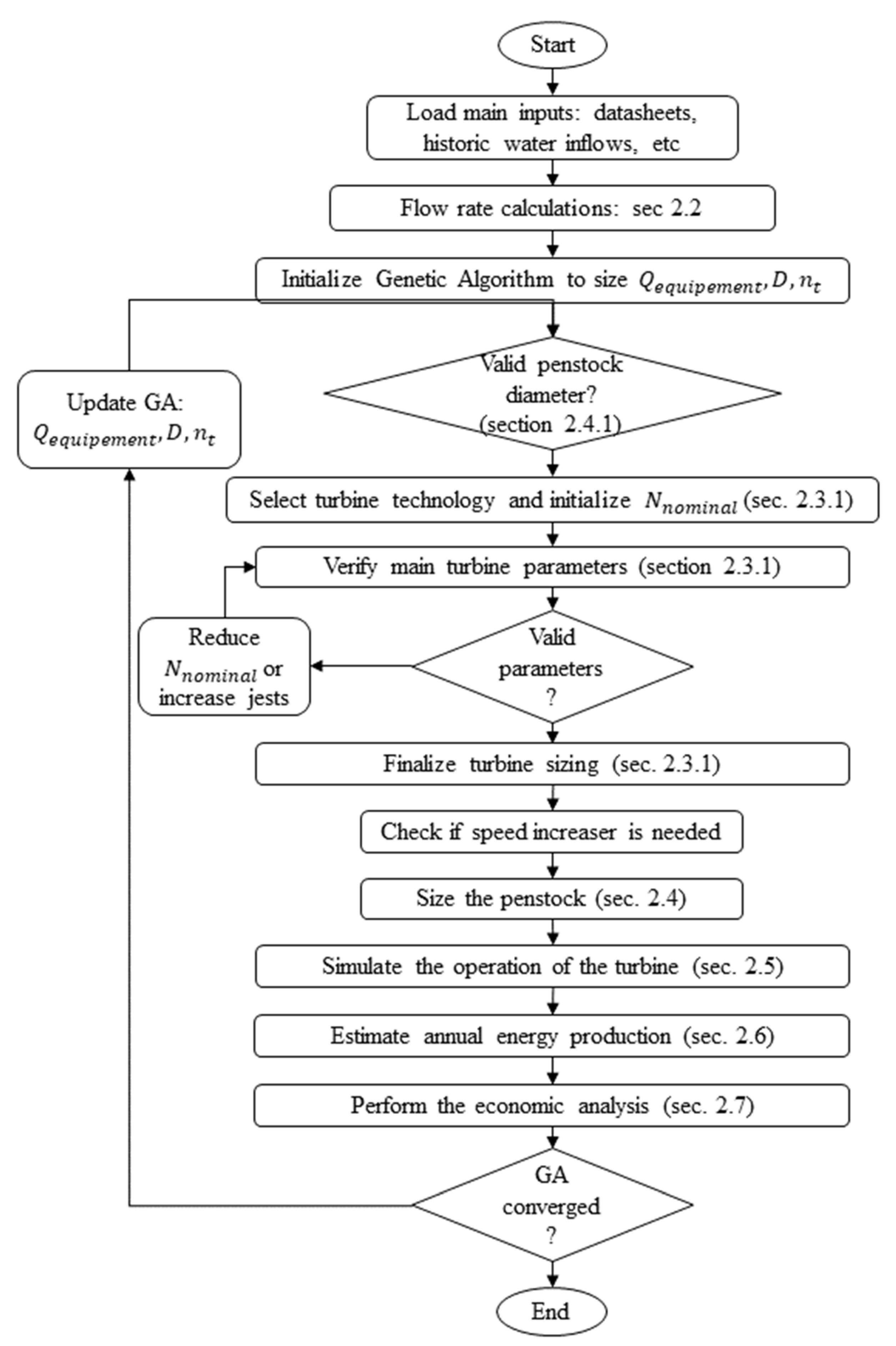
2.1. The Design Procedure

In general, the design of a small run-of-river hydropower plant relies on the technical knowledge and experience of hydropower engineers, supported by mathematical tools to support the analysis that may approximate the large number of possibilities depending onsite-specific conditions [41]. Based on a number of hypotheses, this study proposes a numerical model for the LCOE-based optimization of the design of a small run-of-river hydroelectric power plant with the aim of simplifying the pre-feasibility studies for this type of project. This numerical model aims at providing approximate general results to support a preliminary feasibility study for a site using a limited number of information, up to only the average daily flows and the gross head.

The assumptions on which the numerical model is based are as follows:

• Penstocks are buried only if a minimum of rock excavation is required [41]. However, since excavation leads to additional costs, this study assumes that penstocks are installed over the ground, hence leading to a positive suction head;
• The plant is connected to an existing electrical network and, hence, all the electricity produced is actually sold;
• The power plant is always in operation: no fault occurs, and as multiple turbines are installed, it is assumed that the maintenance plan can be performed without interruptions;
• Line losses are neglected;
• In order to generalize the model, the penstock configuration and its singularities are understood as sufficiently close to those of the 21 power plants that allowed Singhal MK and Arun Kumar [23] to develop a relationship between total head losses and friction losses: this formula allows one to calculate total head losses from friction losses, penstock length, and gross head and was found to be usable for hydropower projects due to the correlation coefficient of the relation obtained being 0.837, which is within the authorized limit;
• The deviation of the watercourse is made from a weir that does not allow considerable storage, as the role of the retaining structure is only to keep the level constant so as to ensure that the water intake and penstock are always supplied [41]. Additionally, that it is set up with what is necessary for the normal operation of the power plant, for example, it should be able to prevent the entry of suspended sediments;
• The topography of the site is appropriate for the production of hydroelectricity;
• The gross head is constant and that when dealing with low head schemes (2–30 m), since this assumption is no longer verified, an average value of the gross head measured is used;
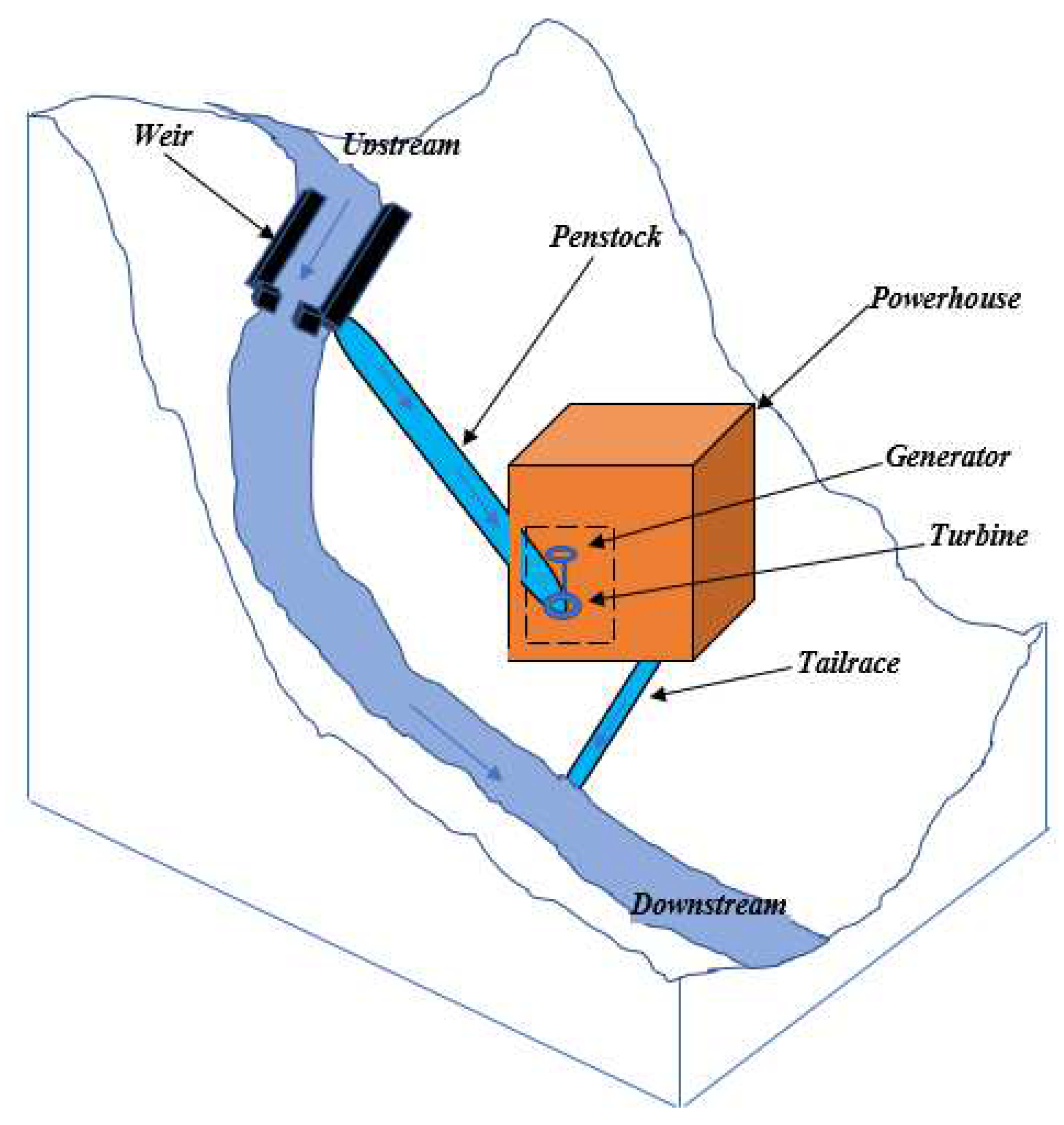
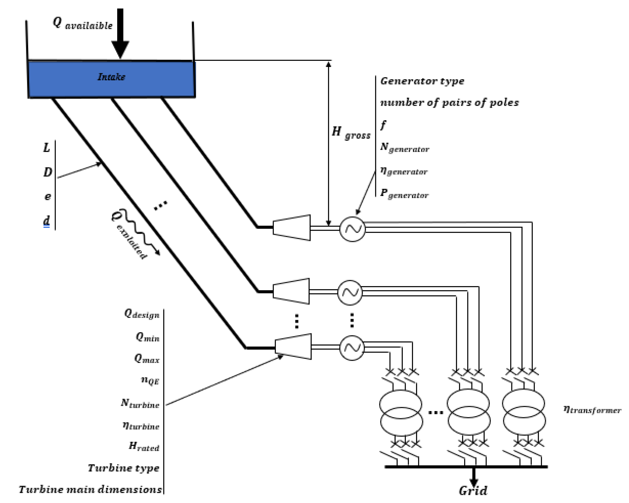
• The numerical model focuses on small run-of-river hydropower plants with a capacity between 500 kW and 10 MW, therefore having low- and high-head projects (3–20 m and above 100 m) and for a configuration where the intake is directly linked to the penstock, as shown in Figure 1.

Thus, the procedure used to design the run-of-river project is as follows:

• Design of the penstock: calculation of its diameter, its thickness, and its aeration pipe diameter;
• Determination of the optimal number of turbines;
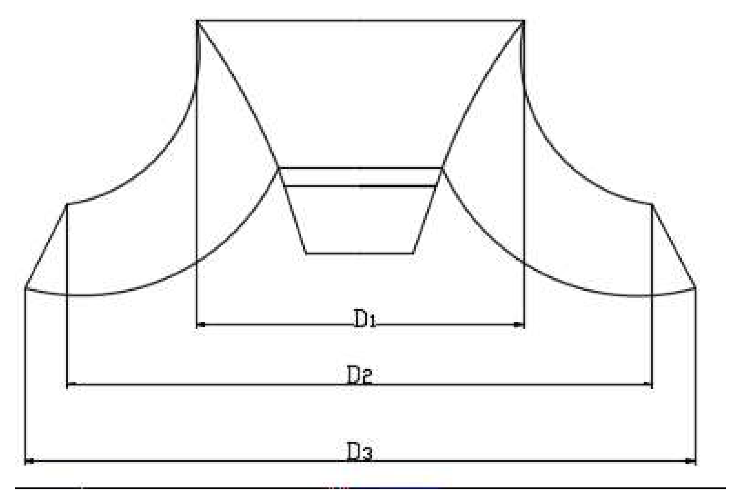
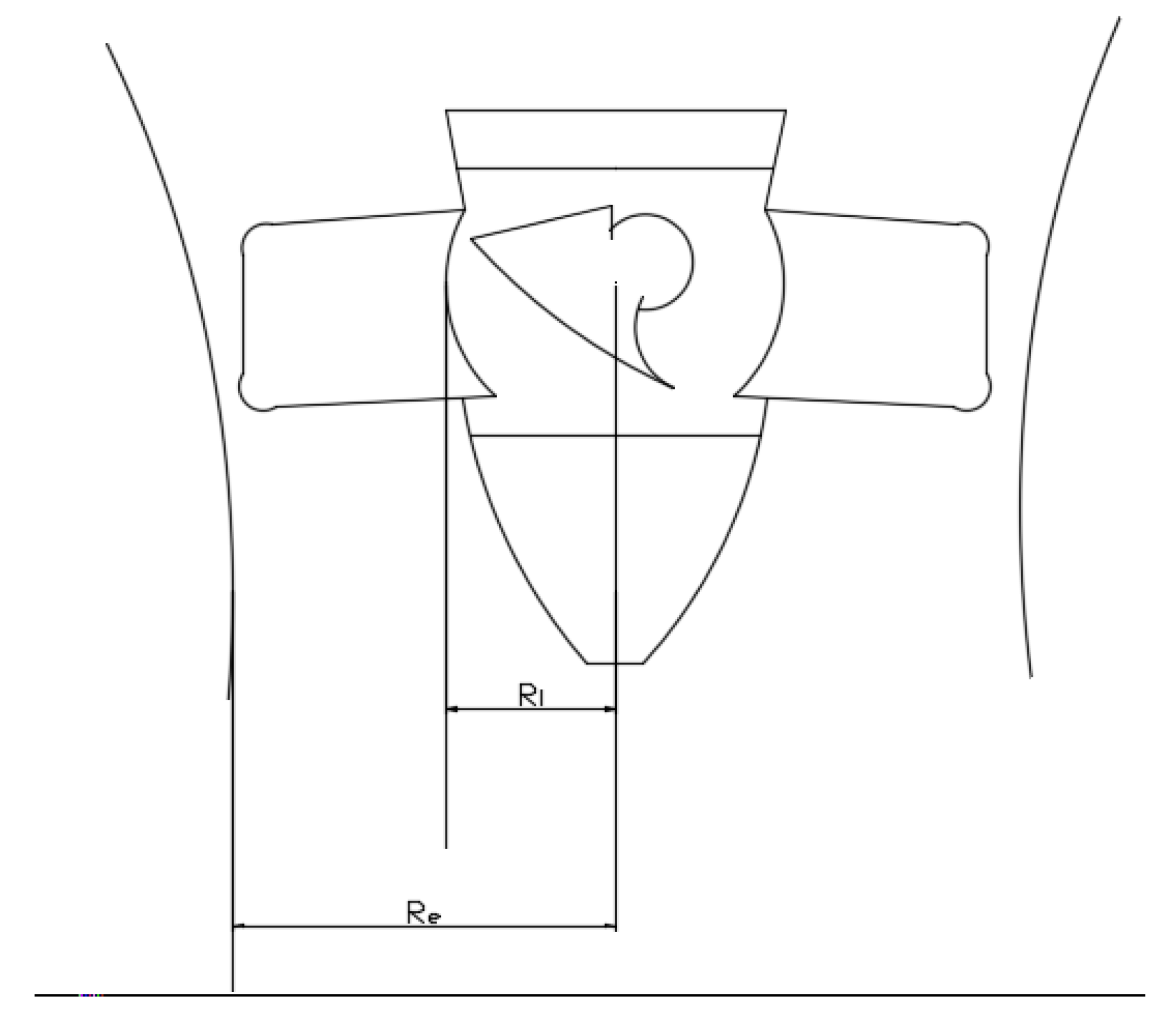
• Optimal selection of turbine: turbine type, admissible suction head, design flow rate, rated head, rated power, rotational speed, specific speed, and main dimensions of the turbine wheels;
• Choice of generator: type of generator, frequency, number of pairs of poles, rated power, and rotation speed;
• Choice of whether or not to use a speed increaser between the turbine and the generator;
• Estimate of the annual energy produced;
• Estimation of the investment, operating, and maintenance costs of the project over its lifetime;
• Calculation of economic criteria: LCC, LCOE, Net Present Value, and return on investment time;
• Choice of the technical solution with the best LCOE;
• Simulation of the operating mode of the sized run-of-river plant equipment (penstocks, turbines, and generators), thus making it possible to estimate the average daily flow rates driving each turbine; the number of turbines used each day of the year; the average daily speeds of water in the penstock; friction; singular and total average daily head losses in the penstock; the average daily net heads; and average daily energies produced.

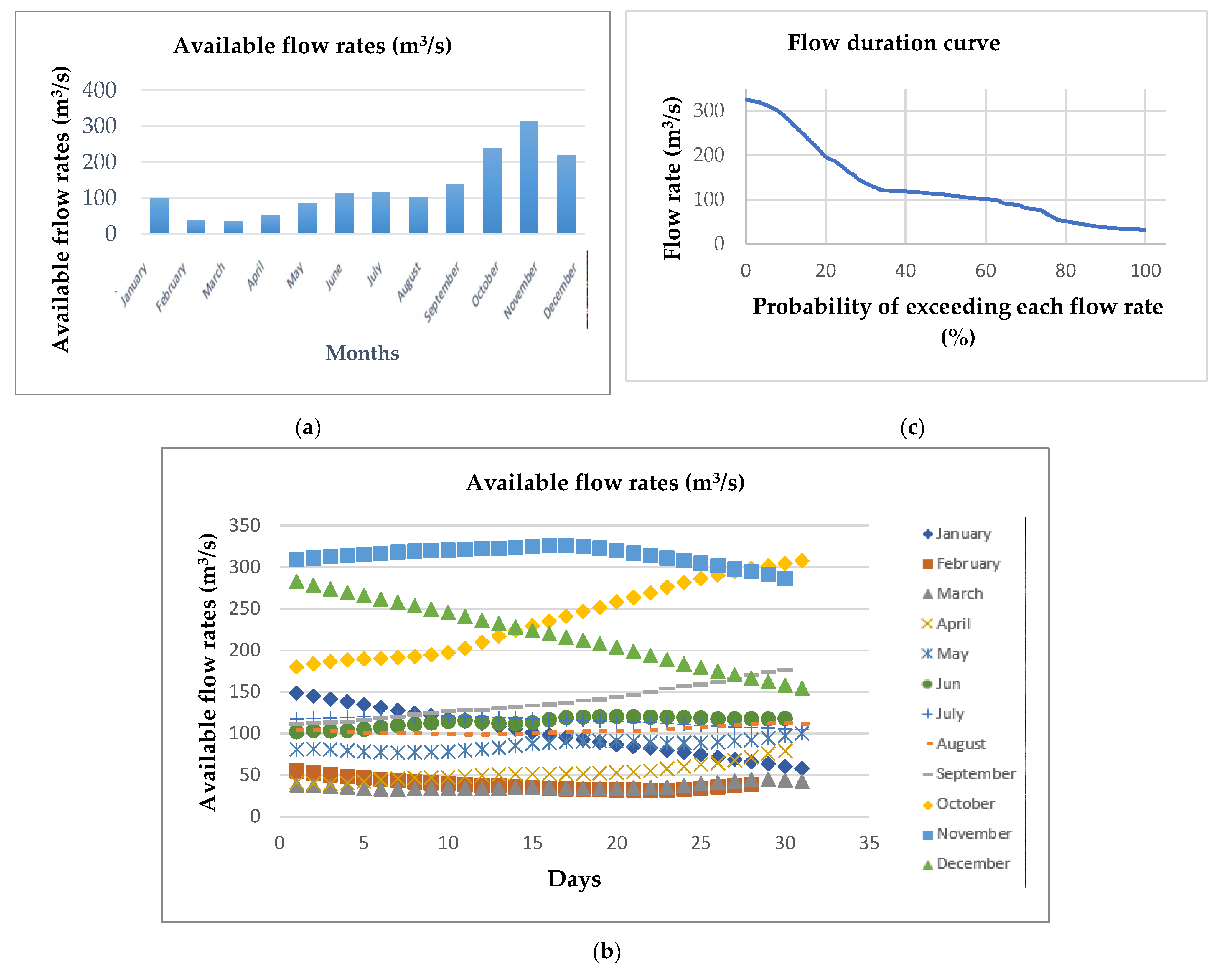
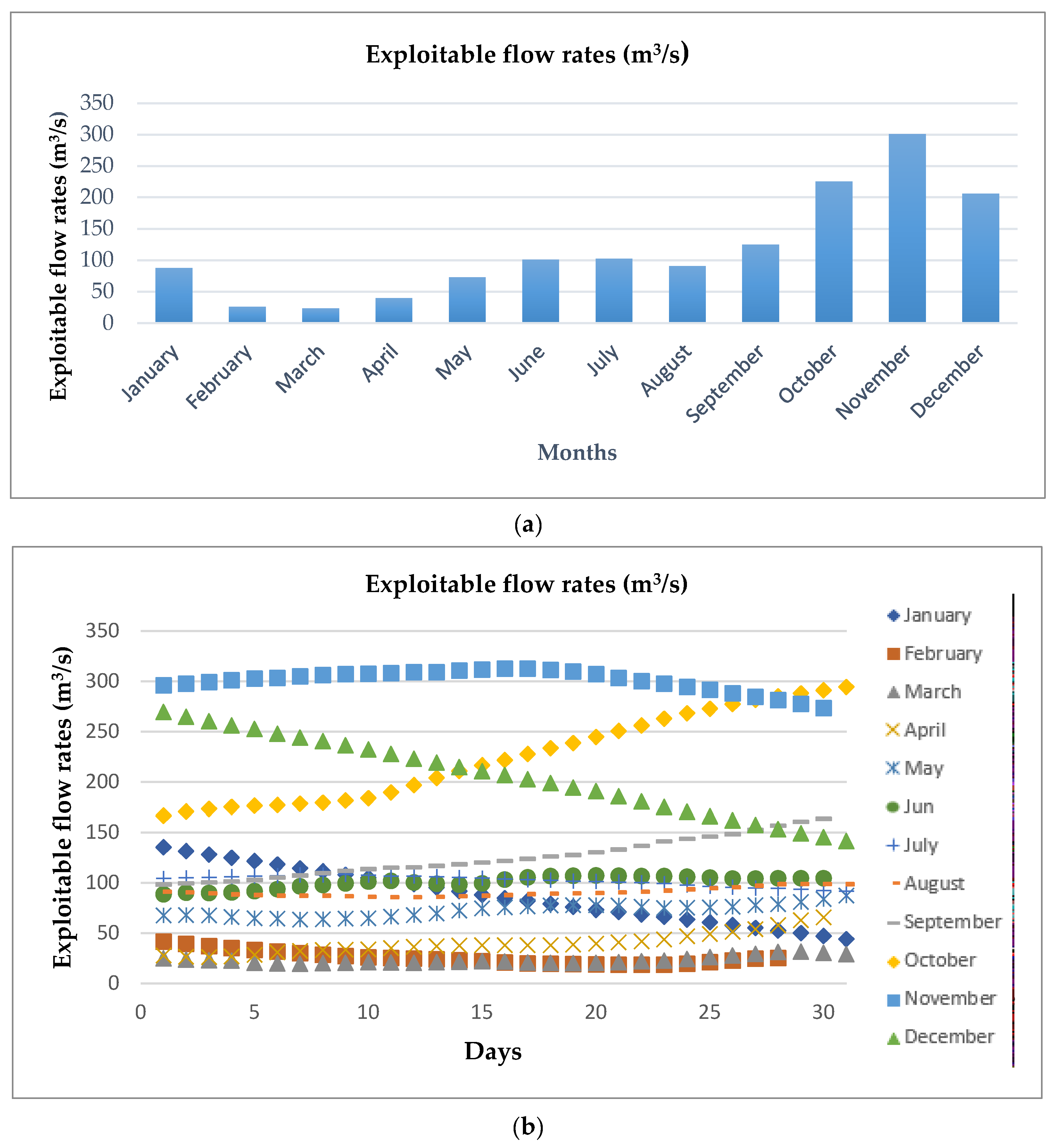
2.2. Definition of the Flow Rate of the Equipment

The flow of equipment is the maximum flow that can be carried by the installation without causing unacceptable losses; further, the flow rate of equipment is set from the flow duration curve [42,43,44].

According to several authors [43,44], the choice of the flow rate of equipment also depends on the type of application, be it a standalone system or connected to the grid. This is the reason why the flow rate of equipment here will be a flow between the 25th (Q_25) and 15th (Q_15) quartiles of the flow, as recommended by Hanggi and Weingartner [44].

The flow duration curve will be obtained by ranking the daily flow rates from largest to smallest, and by calculating the probability of exceeding each flow rate with the formula below [45]:

$$P=\frac{m}{N+1}\times 100\%$$

(1)

where m is the rank of the flow in the classification made above, and N the total number of recorded flows (which in our case is 365 because this study is dealing with average daily flows).

2.3. Selection of Turbine and Generator Technology

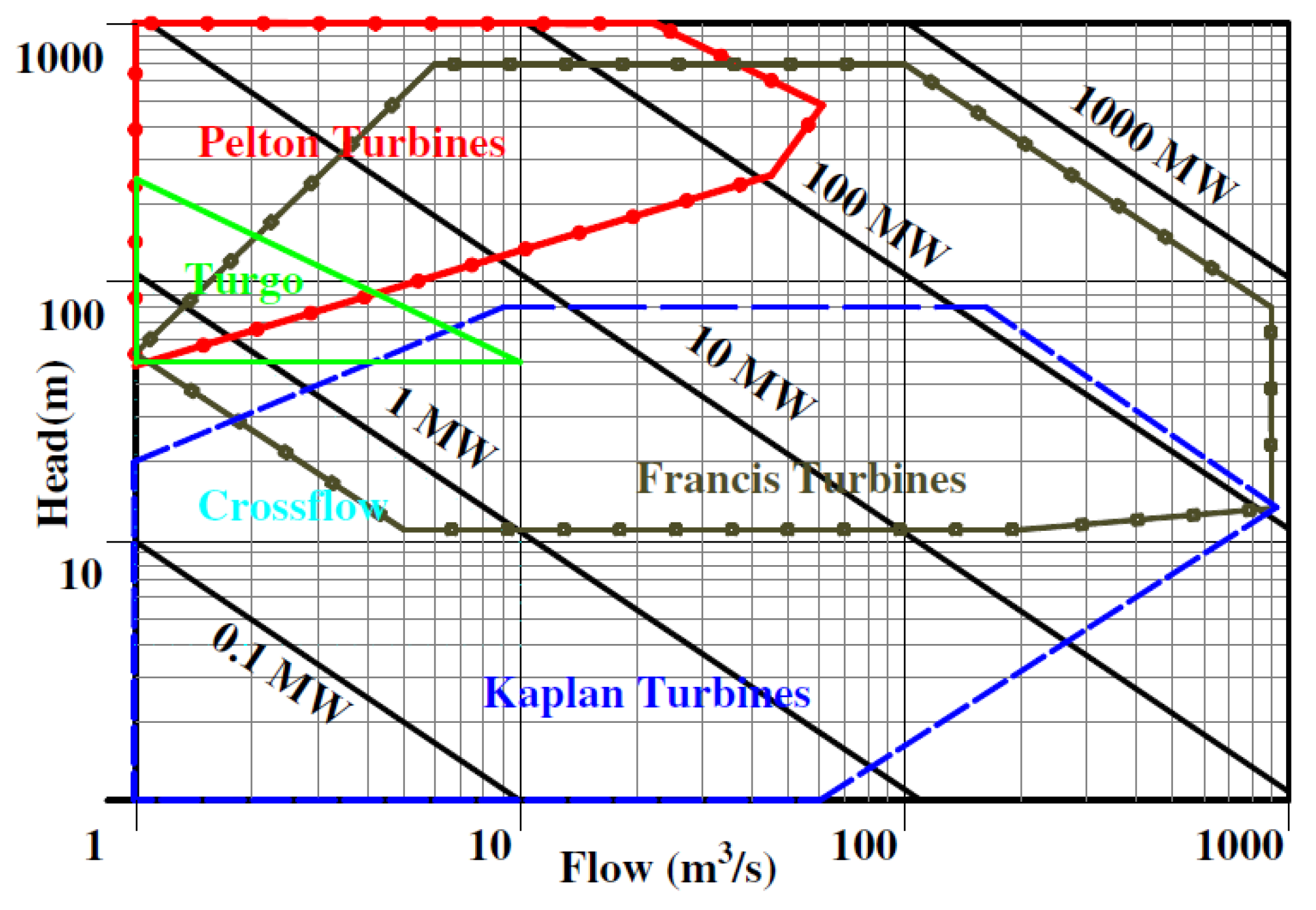
2.3.1. Turbine Case

The type of the turbine can be preliminarily chosen based on the chart in Figure 2, provided the design flow rate, which is calculated before, and the rated head of the study site.

As can be seen on the chart above, there are situations in which the values of the design flow rate and the rated head of the study site could refer to several types of turbine. Kaplan, Francis, and Pelton are the only types of turbine considered here because they are the turbine technologies with the best efficiencies; thus, often a choice has to be made between them. Since according to

Table 1. Flow and head variation acceptance [41].

Turbine Type	Acceptance of Flow Variation	Acceptance of Head Variation
Pelton	High	Low
Francis	Medium	Low
Kaplan double regulated	High	High
Kaplan single regulated	High	Medium
Propeller	Low	Low

, Pelton and Kaplan turbines better handle fluctuations in the flow and head; as such, they may often be preferred.

Once the type of turbine is chosen, the minimum and maximum rotation speeds of the turbine can be calculated using

Table 2. Ranges of the specific speed of each type of turbine [41].

Type of Turbine	Range
Pelton one nozzle	0.005 ≤ $n_{QE}$ ≤ 0.025
Pelton n nozzles	0.005 n0.5 ≤ $n_{QE}$ ≤ 0.025 n0.5
Francis	0.05 ≤ $n_{QE}$ ≤ 0.33
Kaplan, propellers, bulbs	0.19 ≤ $n_{QE}$ ≤ 1.55

and Formula (2):

$$n=\frac{n_{QE}.{\left(g{H}_{rated}\right)}^{3/4}}{\sqrt{Q_{design}}}$$

(2)

where n is the speed of rotation of the turbine in rpm, n_QE the specific speed of the turbine, g the acceleration of gravity in m/s², H_rated the rated head in m, and Q_design the design flow rate of the turbine in m³/s.

Then, this study initially takes, as the speed of rotation of the turbine, the standard speed of

Table 3. Generator synchronization speed.

Number of Poles	Speed for a Frequency of 50 Hz (rpm)
2	3000
4	1500
6	1000
8	750
10	600
12	500
14	428
16	375
18	333
20	300
22	272
24	250
26	231
28	214

as directly lower than the maximum speed calculated above.

Finally, the specific speed n_QE and the maximum admissible suction head H_s, in the case of reaction turbines, can be calculated using Equations (2) and (3) [41]:

$$H_S=H_a-H_v+\frac{V^2}{2g}-{\sigma }_{turbine type} H_{rated}$$

(3)

In Equation (3), σ will be calculated from Equations (4) and (5) where V = 2 m/s, as is recommended by ESHA [41].

$${\sigma }_{Kaplan}=1.5241n_{QE}{}^{1.46}+\frac{V^2}{2gH}$$

(4)

$${\sigma }_{Francis}=1.2715n_{QE}{}^{1.41}+\frac{V^2}{2gH}$$

(5)

If the maximum admissible suction head is negative, an excavation is necessary (additional civil works), which would increase the costs of the project. To avoid this, there is the need to change the speed of rotation for the turbine to obtain a non-negative value of the maximum admissible suction head. If no standard rotation speed in the table allows a positive maximum admissible suction head to be obtained, the problem can still be resolved in the optimization process, through the selection of a flow rate of equipment allowing one to respect this constraint (through the design flow rate).

The main dimensions of the turbine wheels are also estimated in order to further guide the choice.

• Pelton turbines

With the rotational speed of the runner of a Pelton turbine, the diameter can be calculated by the following equations [41]:

$$D_1=0.68\frac{\sqrt{H_{rated}}}{n}$$

(6)

$$B_2=1.68\sqrt{\frac{Q_{design}}{n_{jet}}.\frac{1}{\sqrt{H_{rated}}}}$$

(7)

$$D_e=1.178\sqrt{\frac{Q_{design}}{n_{jet}}.\frac{1}{\sqrt{H_{rated}}}}$$

(8)

where n is the rotational speed in rpm, n_jet the number of nozzles, H_rated the rated head in m, and g the gravity constant in m/s².

D₁ is defined as the diameter of the circle describing the bucket’s center line in m. B₂ is the bucket width in m, which is mainly dependent on the flow rate and the number of nozzles. D_e is the nozzle diameter in m.

Generally, the inequality of D₁/B₂ >2.7 should always hold; otherwise, a new calculation with a lower rotational speed or a higher number of nozzles will have to be carried out [41].

• Francis turbines

The reference diameters of a Francis runner can be estimated using Equations (9)–(11), where their nomenclature is highlighted in Figure 3 [41]:

$$D_3=84.5\left(0.31+2.488n_{QE}\right)\frac{\sqrt{H_{rated}}}{60n}$$

(9)

$$D_1=\left(0.4+\frac{0.095}{n_{QE}}\right)D_3$$

(10)

The inlet diameter is given by the equation below for n_QE > 0.164 [41]:

$$D_2=\frac{D_3}{0.96+0.3781n_{QE}}$$

(11)

For 0.164 > n_QE: D₁ = D₂.

• Kaplan turbines

The reference diameters of a Kaplan runner are reported in the Equations (12) and (13), then highlighted in Figure 4 [41]:

$$D_e=84.5\left(0.79+1.602n_{QE}\right)\frac{\sqrt{H_{rated}}}{60n}$$

(12)

$$D_i=\left(0.25+\frac{0.0951}{n_{QE}}\right).D_e$$

(13)

At this level, based on the speed of rotation of the turbine, it is also possible to estimate whether a speed increaser is necessary. According to ESHA [41], a speed increaser will be used only to interface turbines with a rotational speed of less than 428.57 rpm and standard alternators with nominal rotating speeds between 750 and 1500 rpm.

The remaining characteristics of the turbine can be calculated using the formulas below:

$$H_{rated}=H_{min}=0.96H_{gross}$$

(14)

$$P_{turbine}={\eta }_{turbine}g{Q}_{design}{H}_{rated}$$

(15)

with:

P_turbine: Rated power of the turbine (kW);

η_turbine: Rated efficiency of the turbine (-);

H_rated: Rated head of the turbine (m);

H_min: Minimal net head of the turbine (m);

H_gross: Gross head of the turbine, which is the difference between the upstream and the downstream level for reaction turbines and also the difference between the upstream and the downstream level minus the height of the nozzle jet above the tail race, which is fixed at 1 m here for impulse turbines [15] (m);

Q_design: Design flow rate of the turbine (m³/s);

Q_equipement: Flow rate of equipment of the plant (m³/s);

n_t: Number of turbines (-).

The expected rated efficiency of the turbine can be estimated using

Table 4. Typical efficiencies of small turbines [41].

Turbine Type	Best Efficiency
Kaplan single regulated	0.91
Kaplan double regulated	0.93
Francis	0.94
Pelton n nozzles	0.9
Pelton 1 nozzle	0.89
Turgo	0.85

.

2.3.2. Generator Case

First, since this study deals with the design of a run-of-river hydroelectric power plant, the type of generator used will always be asynchronous with a frequency of 50 Hz, as is the case in Cameroon.

As for the generator rotational speed, if no speed increaser is used, the generator will have the same speed as the turbine. Otherwise, a speed of 750 rpm will always be considered. The number of pole pairs can be deduced from Table 3, presented above.

The rated power of the generator is calculated with Formula (16) below:

$$P_{generator}={\eta }_{generator}{\eta }_{increaser}{\eta }_{turbine}g{Q}_{design}{H}_{rated}$$

(16)

where η_generator is the rated efficiency of the generator depending on its rated power, as can be seen in

Table 5. Typical efficiencies of small generators [41].

Rated Power	Best Efficiency
10	0.91
50	0.94
100	0.95
250	0.955
500	0.96
1000	0.97

, and η_increaser is the efficiency of the speed increaser set at 0.97 (as according to ESHA [41], its efficiency varies from 0.96 to 0.98) and η_turbine is the rated efficiency of the turbine.

2.4. Design of the Penstock

2.4.1. Calculation of the Penstock Diameter

To calculate the optimal diameter, first, the maximum speed interval needs to be quantified in relationship with the head for the case study, which is given in

Table 6. Maximum speed in penstock according to the head [47].

Head (m)	Maximum Speed (m/s)
Low head (50 < H)	2–3
Medium head (50 ≤ H ≤ 250)	3–4
High head (H > 250)	4–5

.

Then, provided the maximum and minimum speeds apply as shown in Table 6, the maximum and minimum diameter of the penstock can be determined with Equations (17) and (18):

$$D_{min}=\sqrt{\frac{4Q_{design}}{V_{max}\pi }}$$

(17)

$$D_{max}=\sqrt{\frac{4Q_{design}}{V_{min}\pi }}$$

(18)

Once these bounds are calculated, the diameter of the interval that allows having the best value of the objective function shall be calculated by using an optimization algorithm, which will be presented in the next few subsections.

2.4.2. Calculation of the Penstock Thickness

To determine the thickness of the penstock, the three methods presented below can be used. Further, it is the maximum value, among the three values obtained from the three methods, that should be taken.

The first method uses the iterative procedure presented below [48]:

• Proposal of a first estimate of e
• Calculate c, h_max, and e_min
• Compare e and e_min: if e < e_min, then start again with a larger value of e and e > e_min. Attempt to make e equal to the available wall thickness that is closest to e_min, above or below, and repeat the calculation.
• Repeat the two previous steps until the minimum available wall thickness is made to be greater than e_min
• e should be increased by 1.5 mm while dealing with mild steel pipes in order to take into consideration corrosion effects.

The parameters mentioned above are calculated with the equations below:

$$h_{surge}=\frac{CV }{g}$$

(19)

$$C=\frac{1}{\sqrt{\rho \left(\frac{1}{k}+\frac{D}{Ee}\right)}}$$

(20)

$$e_{min}=\frac{\rho g{h}_{max}DF}{2\sigma }$$

(21)

$$H_{max}=H_{gross}+H_{surge}$$

(22)

where

$H_{surge}$: Surge pressure head (m);

$H_{max}$: Maximum possible pressure head experienced by the pipe (m);

$H_{gross}$: Gross head (m);

$C$: Velocity of the pressure wave through the water (m/s);

$V$: Flow velocity with valve fully open (m/s);

$\rho$: Density of water (m³/s);

$k$: Bulk Modulus of water (N/mm²);

$E$: Young’s Modulus of Elasticity for pipe material (N/m²);

$D$: Pipe diameter (mm);

$e$: Pipe wall thickness (mm);

$e_{min}$: Minimal pipe wall thickness (mm);

$g:$ Gravitational acceleration (m/s²);

$F$: Safety factor, typically 3;

$\sigma$: Ultimate tensile strength of pipe material (N/mm²);

The two other methods rely, respectively, on the two equations given below and are used to estimate the minimum wall thickness that will make the penstock rigid enough to be handled without danger of deformation in the field [41]:

$$e_{\min }=2.5D+1.2$$

(23)

where $D$ is the diameter in m.

$$e_{\min }=\frac{D+508}{400}$$

(24)

where $D$ is the diameter in mm.

2.4.3. Calculation of the Air Vent Pipe Diameter

According to ESHA [41], a penstock can collapse due to high depression. The maximum negative depression the material can withstand is given by the formula below (in kN/mm²):

$$P_C=882500{\left(\frac{e}{D}\right)}^3$$

(25)

When an aeration pipe is installed, the diameter can be reduced as described in (26) [42]:

$$d=7.47\sqrt{\frac{Q_{design}}{\sqrt{P_C}}}$$

(26)

for $P_C\le 0.49$ kgN/mm².

Otherwise, the minimum recommended diameter shall be computed using (27)

$$d=8.94\sqrt{Q_{design}}$$

(27)

2.5. Turbine Operation Model

For the simulation of the turbine operation, not only are the minimum and the maximum flow rates of the turbine, respectively $Q_{min} \mathrm{and} Q_{max}$, considered, but also the safety flow rate $Q_{safety} ,$ which is the maximum operational flow of the hydroelectric power plant. The safety flow rate is an important parameter because, according to Hanggi and Weingartner [44], if the flow exploited by the power plant is greater than $Q_{safety}$, then the plant may suffer from damage.

This flow will be the one with an exceedance probability of 2%, as proposed by Hanggi and Weingartner [44]. Since this study proposes a model of a power plant with several identical turbines ($n_t)$, for a more efficient use of the hydraulic resource, based on the constraints presented above, this study uses the following operating algorithm:

$$Q_{\mathrm{exploited}}\left(j\right) =\{\begin{array}{c}0 if Q_{exploitable}\left(j\right) <Q_{min } \left(1\right)\\ Q_{exploitable }\left(j\right) if Q_{min} \le Q_{exploitable}\left(j\right)\le Q_{max} \left(2\right)\\ Q if Q_{max}<Q_{exploitable}\left(j\right)\le n_t{Q}_{max} \left(3\right)\\ n_t{Q}_{max} if n_t{Q}_{max}<Q_{exploitable}\left(j\right)<Q_{safety} {\left(4\right)}_{ }\\ 0 if Q_{exploitable}\left(j\right) \ge Q_{safety } \left(5\right)\end{array}$$

(28)

• In the first case (1), no turbine is in operation;
• In case (2), a turbine is in operation, and this is all the exploitable flow that is used;
• In case (3), (x + 1) turbines operate such that $Q=y.\left(x+1\right).Q_{max}$ with 0 $\le$ y $\le 1$ and (x + 1), which is the natural number directly greater than $Q/Q_{max}$ ($x\le Q/Q_{max}\le x+1$), if $Q_{min }/Q_{max}\le y$ or x turbines operate such that $Q=x.Q_{max}$ if $y<Q_{min }/Q_{max}$;
• In case (4), all the turbines are in rated operation, each of them exploiting the maximum flow that it can turbinate and the rest of the water flow $Q_{turbinable}-n_t{Q}_{max}$ being lost;
• In case (5), no turbine is operating.

The minimum flow $Q_{residual }$, which cannot be used for environmental reasons, is here assumed to be 10% of the interannual flow of the watercourse in order to produce a project that is more respectful of the environment [41].

This leads to:

$$Q_{exploitable}\left(j\right)=Q_{availabl}{}_e\left(j\right)-Q_{residual}=Q_{available}\left(j\right)-0.1Q_{interannual}$$

(29)

where $Q_{exploitable }$ is the exploitable flow rate in m³/s, $Q_{exploited }$ is the exploited flow rate in m³/s, $Q_{available }$ is the available flow rate in m³/s, and $Q_{interannual }$ is the average daily flow rate available over the year in m³/s.

The formulas for the calculation of the daily average values of the head losses, and the net head, for each day j of the year are presented below [23]:

$$V\left(j\right)=\frac{4Q_{exploited}\left(j\right)}{D^2\pi }$$

(30)

$$\mathrm{\Delta }{H}_{friction}\left(j\right)=\frac{\lambda V{\left(j\right)}^{2}L}{2Dg}$$

(31)

$$\mathrm{with} \frac{1}{\sqrt{\lambda \left(j\right)}}=-2lo{g}_{10}\left(\frac{\epsilon }{3.7D}+\frac{2.51}{R_e\left(j\right)\sqrt{\lambda \left(j\right)}}\right)$$

(32)

$$\mathrm{and} R_e\left(j\right)=\frac{V\left(j\right)\mathrm{D} }{\nu }$$

(33)

$$\mathrm{\Delta }{H}_{ total}=2.644{(\frac{L}{H_{gross}})}^{-0.19}\mathrm{\Delta }{H}_{friction}\left(j\right)$$

(34)

$$\mathrm{\Delta }{H}_{singular}\left(j\right) =\mathrm{\Delta }{H}_{total}\left(j\right)- \mathrm{\Delta }{H}_{friction }\left(j\right)$$

(35)

$$H_{net}\left(j\right)=H_{gross}-\mathrm{\Delta }{H}_{total}\left(j\right)$$

(36)

$H_{gross}:$ Gross head (m);

$H_{net}\left(j\right):$ Net head of the day j (m);

$\mathrm{\Delta }{H}_{friction }\left(j\right)$: Friction loss of the day j (m);

$\mathrm{\Delta }{H}_{singular}\left(j\right)$: Singular losses of the day j (m);

$\mathrm{\Delta }{H}_{total}\left(j\right):$ Total head loss of the day j (m);

$\lambda \left(j\right):$ Friction factor of the day j (-);

$V\left(j\right):$ Flow velocity the day j (m/s);

$L:$ Length of the penstock (m);

$D:$ Diameter of the penstock (m);

$g:$ Gravitational acceleration (m/s²);

$\epsilon :$ Roughness heigh for welded steel (mm);

$\nu :$ Kinematic viscosity of water (m²/s);

$R_e \left(j\right):$ Reynolds number of the day j (-);

$Q_{exploited}\left(j\right)$: Exploited flow rate of the day j (m³/s).

In the same way, the average daily powers and energies can also be estimated with the following formulas:

$$P_{hyd}\left(j\right)=g{Q}_{exploited}\left(j\right) H_{net}\left(j\right)$$

(37)

$$P_{meca}\left(j\right)={\eta }_{turbine}\left(j\right)P_{hyd}\left(j\right)$$

(38)

$$P_{elec}\left(j\right)={\eta }_{transformer}\eta {^}_{generator}{P}_{meca}\left(j\right)$$

(39)

$$E_{elec}\left(j\right)=24P_{elec}\left(j\right)$$

(40)

$P_{hyd}\left(j\right):$ Hydraulic power of the day j (kW);

$P_{mec}\left(j\right):$ Mechanical power of the day j (kW);

$P_{elec}\left(j\right):$ Electrical power of the day j (kW);

$E_{elec}\left(j\right):$ Electrical energy of the day j (kWh);

${\eta }_{turbine}\left(j\right):$ Efficiency of the turbine the day j (-);

$\eta {^}_{generator}:$ Average efficiency of the generator set to 0.9 (-);

${\eta }_{transformer}$: Average efficiency of the transformer set to 0.98 (-) [49].

The hydro turbines efficiencies for each day j are calculated through the equations below depending on parameters such as the rated head, the runner diameter, the turbine specific speed, and the turbine manufacturer/design coefficient [50]:

$${\eta }^{^}{}_{Kaplan/peak}=\left(0.905-{\eta }^{^}{}_{kaplan/nq}+{\eta }^{^}{}_d\right)-0.0305+0.005R_m$$

(41)

$${\eta }^{^}{}_{kaplan/nq}={\left(\left({\eta }_q-170\right)/700\right)}^2$$

(42)

$${\eta }^{^}{}_{kaplan /d}=\left(0.095+{\eta }^{^}{}_{kaplan/nq} \right)\left(1-0.789 d^{-0.2}\right)$$

(43)

$${\eta }^{^}{}_{Kaplan}\left(j\right)=\left[1-3.5{\left(\frac{Q_{P/kaplan}-Q\left(j\right)}{Q_{P/kaplan}}\right)}^6\right]{\eta }^{^}{}_{Kaplan/peak}$$

(44)

$$d=K{Q}_{design}{}^{0.473}$$

(45)

$$n_q=k{H}_{rated}{}^{-0.5}$$

(46)

$${\eta }^{^}{}_{francis/peak}=\left(0.919-{\eta }^{^}{}_{francis/nq}+{\eta }^{^}{}_{francis/d}\right)-0.0305+0.005R_m$$

(47)

$${\eta }^{^}{}_{francis/nq}={\left(\left({\eta }_q-56\right)/256\right)}^2$$

(48)

$${\eta }^{^}{}_{francis /d}=\left(0.081+{\eta }^{^}{}_{francis/nq} \right)\left(1-0.789 d^{-0.2}\right)$$

(49)

$${\eta }^{^}{}_{francis/below}\left(j\right)=\left[1-\left[1.25{\left(\frac{Q_{P/francis}-Q\left(j\right)}{Q_{P/francis}}\right)}^{\left(3.94-0.0195n_q\right)}\right]\right]{\eta }^{^}{}_{francis/peak}$$

(50)

$${\eta }^{^}{}_{francis/above}\left(j\right)={\eta }^{^}{}_{francis/peak}-\left[{\left(\frac{Q\left(j\right)-Q_{P/francis}}{Q_{design}-Q_{P/francis}}\right)}^2\left({\eta }^{^}{}_{francis/peak}-{\eta }^{^}{}_{francis/r}\right)\right]$$

(51)

$${\eta }^{^}{}_{francis/p}=0.0072n_q{}^{0.4}$$

(52)

$${\eta }^{^}{}_{francis/r}=\left(1-{\eta }^{^}{}_{francis/p}\right){\eta }^{^}{}_{francis/peak}$$

(53)

$$n=31{\left(H_{rated}\frac{Q_{design}}{j}\right)}^{0.5}$$

(54)

$$d_{out}=\frac{49.4H_{rated}{}^{0.5}{j}^{0.02}}{n},$$

(55)

$${\eta }^{^}{}_{pelton/peak}=0.864 d_{out}{}^{0.04},$$

(56)

$${\eta }^{^}{}_{pelton}\left(j\right)=\left[1-\left[\left(1.31+0.025j\right){\left|\left(\frac{Q_{P/pelton}-Q\left(j\right)}{Q_{P/pelton}}\right)\right|}^{\left(5.6+0.4J\right)}\right]\right]{\eta }^{^}{}_{pelton/peak},$$

(57)

where:

${\eta }^{^}{}_{Kaplan}\left(j\right)$ is the efficiency of Kaplan turbines at a flow above or below peak efficiency and

${\eta }^{^}{}_{turbine type/peak}$ is the turbine peak efficiency of the turbine type considered.

$Q_{P/turbine type }$ is the peak efficiency flow of the turbine type considered (=$0.75Q_{design} for Kaplan,=0.65Q_{design}{n}_q{}^{0.05}for Francis turbine and=\left(0.662+0.001j\right)Q_{design} for pelton)$.

${\eta }^{^}{}_{turbine type/d}$ is the runner size adjustment to peak efficiency of the turbine type considered.

${\eta }^{^}{}_{turbine type/nq}$ is the specific speed adjustment to peak efficiency of the turbine type considered.

$Q_{design}$ is the design flow rate;

$n_q$ is the specific speed based on flow;

$k$ = 800 for Kaplan turbines and 600 for Francis turbines;

$H_{rated}$ is the rated head on turbine in m;

$d$ is the runner throat diameter in m;

$K$ = 0.46 for $d<$1.8 and $K$ = 0.41 for $d\ge$1.8;

$R_m$ is the turbine manufacturer/design coefficient (2.8 to 6.1; default = 4.5);

$j$ is the number of jets while dealing with Pelton turbines;

$n$ is the rotational speed of Pelton turbines;

$d_{out}$ is the outside diameter of runner of Pelton turbines.

The Figure 5 below shows the general configuration of the small run-of-river hydropower plant proposed by our methodology with all the parameters characterizing each of the component taken into account in our case and whose models are presented above.

2.6. Annual Energy Production Estimation

Since, in this study, several turbines are considered, including their alternators and their penstock, it must be stressed that they will not always be working all at the same time. The operating forecasts of these turbines can therefore make it possible to set up a maintenance schedule for electromechanical equipment, which would prevent downtime for maintenance.

Thus, this study first assumes that the power plant is always in operation (it never experiences any downtime).

$$E_{elec annual}={\displaystyle \sum }_{j=1}^{365}24P_{elec}\left(j\right)$$

(58)

$E_{elec annual}$: Productible annual electrical energy (kWh);

$P_{elec}\left(j\right)$: Electrical power of the day j (kW).

2.7. Economic Analysis

Economic analysis is the phase following the design of the plant and thus allowing the assessment of the profitability of the project. Costs of small hydropower projects include fixed and variable cost. Fixed costs include expenditures due to civil works and electromechanical equipment, while the variable costs take into consideration replacement, operation, and maintenance costs [33,50].

2.7.1. Cost Estimate Model

The equations of the model used for the estimation of the investment cost of the project are presented below:

• For a low-head project (3–20 m) [33]

$$Cost of power house building: C_1=92615P^{-0.2351}{H}^{-0.0585},$$

(59)

$$Cost of diversion weir \& intake: C_2=12415P^{-0.2368}{H}^{-0.0597},$$

(60)

$$Cost of penstock: C_3=\pi \left(D+2e\right)e\rho Lpri{x}_{penstock}/\left(P.\mathsf{Ě}\right),$$

(61)

$$Cost of tail race channel: C_7=28164P^{-0.376}{H}^{-0.624}$$

(62)

Finally, the cost in Indian rupees per kilowatt of civil works is $C_C=C_1+C_2+C_3+C_7$

$$Cost of turbines with governing system: C_8=63346P^{-0.1913}{H}^{-0.2171}$$

(63)

$$Cost of generator with excitation system: C_9=78661P^{-0.1855}{H}^{-0.2083}$$

(64)

$$Cost of electrical \& mechanical auxiliaries:C_{10}=40860P^{-0.1892}{H}^{-0.2118}$$

(65)

$$Cost of transformer \& switchyard equipment: C_{11}=18739P^{-0.1803}{H}^{-0.2075}$$

(66)

Finally, the cost in Indian rupees per kilowatt of electromechanical equipment is

$$C_{e\&m}=C_8+C_9+C_{10}+C_{11}$$

(67)

where P is the rated power capacity in kW, H is the rated head in m, D is the penstock diameter in m, e is the thickness of the penstock in m, ρ is the density of welded steel in m³/s, L is the length of the penstock in m, $\mathsf{Ě}$ is Indian rupee/USD rate exchange and Prix_penstock is the cost of the penstock in USD/ton.

• For a high-head project (more than 100 m) [32]

For civil works components, the equations below are used:

$$\begin{gathered} C_x=1.06\times \left(\frac{E}{W}\times cost of earth work in excavation\right)+\left(Conc.\times \\ cost of Concreting\right)+\left(RS\times cost of Reinforced steel\right)+(SS\times \\ cost of Structural Steel/Material) \end{gathered}$$

(68)

$$C_C=C_W+C_{IC}+C_{DT}+C_{HRC}+C_{FS}+C_P+C_{PH}+C_{TRC}$$

(69)

The equations for the calculation of costs of civil works components presented above are used with

Table 7. Correlations of civil works for run-of-river small hydropower plant scheme [51].

No.	Civil Works Components		Items
			Earth Work in Excavation (m3), E/W	Concreting (m3), Conc.	Reinforcement Steel (MT), RS	Structural Steel/Material (MT), SS
1	Diversion weir		$47.00P^{1.10}$ $H^{-0.99}$	$38.55P^{1.17}$ $H^{-1.16}$	$2.59P^{1.18}$ $H^{-1.15}$	$1.51P^{0.71}$ $H^{-0.67}$
2	Penstock (per meter)	PVC pipe	$0.42P^{0.83}$ $H^{-0.98}$	$0.31P^{0.84}$ $H^{-0.98}$	$0.03P^{0.83}$ $H^{-0.97}$	$0.04P^{1.5}$ $H^{-0.81}$
		GRP pipe				$0.01P^{1.5}$ $H^{-0.85}$
		HDPE pipe				$0.08P^{1.5}$ $H^{-0.80}$
		Steel pipe				$0.05P^{0.83}$ $H^{-0.95}$
3	Tail race channel (per meter)		$0.91P^{0.83}$ $H^{-0.90}$	$1.82P^{0.87}$ $H^{-0.91}$	$0.01P^{0.80}$ $H^{-0.79}$	-
4	Powerhouse building	Pelton/Turgo impulse	$16.09P^{2.46}$ $H^{-1.75}$	$0.00052P^{2.54}$ $H^{-0.42}$	$0.00022P^{4.02}$ $H^{-2.83}$	$0.09P^{4.55}$ $H^{-3.50}$
		Francis	$0.08P^{2.33}$ $H^{-1.33}$	$0.03P^{2.29}$ $H^{-1.32}$	$0.05P^{2.36}$ $H^{-1.34}$	$0.02P^{2.19}$ $H^{-1.26}$

and considering the prices as per schedule of rates prevailing for the year 2012 in India [32].

Thus, the prices used are as follows:

• The price for structural steel (including fabrication, transportation to site, and erection) is 75,000 Indian Rupee/MT;
• The price for M20 grade concrete work in plain cement concrete as well as in reinforced cement concrete, including shuttering, mixing, placing in position, compacting, and curing is 3640 Indian Rupee/m³;
• The price for reinforcement steel bars of iron 500 grade, including cutting, bending, binding, and placing in position is 55,000 Indian Rupee/MT;
• The price for earthwork in excavation with all leads and lifts in ordinary soil is 265 Indian Rupee/m³;
• The price for earthwork in excavation with all leads and lifts in soft rock, where blasting is not required is 330 Indian Rupee/m³;
• The price for earthwork in excavation with all leads and lifts in hard rock, including blasting is 550 Indian Rupee/m³.

For electromechanical equipment, the equations below are used:

$$C_y=a_1{P}^{x_1}{H}^{x_2}$$

(70)

$$C_{e\&m}=C_{TG}+C_{GE}+C_{Aux}+C_{T/F}+C_{SY}$$

(71)

The electromechanical equipment considered and the value of the constants $a_1$, $x_1$, and $x_2$ are presented in

Table 8. Coefficients in cost correlation for electromechanical equipment with different types [51].

No.	Type of Equipment		Coefficients in Cost Correlation
			${\mathit{a}}_1$	${\mathit{x}}_1$	${\mathit{x}}_2$
1	Turbine with governing system (TG)	Pelton	117,313	−0.03	−0.39
		Turgo impulse	145,121	−0.12	−0.24
		Francis	125,354	−0.01	−0.38
2	Generator with excitation system or capacitor bank (GE).	Induction	130,262	−0.19	−0.22
		Synchronous	143,660	−0.18	−0.21
3	Auxiliaries		21,846	−0.19	−0.22
4	Transformer		221	0.11	0.01
5	Switchyard		1.82	0.17	0.93

.

The total project cost includes the cost of civil works, the cost of electromechanical equipment, the cost of various items, and other indirect costs. These miscellaneous and indirect costs—which include the costs of design; indirect costs; models; plants; communication; preliminary charge of preparing the report; survey and investigation; environmental impact assessment; and cost of land—represent 13% of the sum cost of civil works and electromechanical equipment. Thus, the total cost of the project in this case can be calculated through the equation below:

$$C_{total}=1.13P.\mathsf{Ě}\left(C_{civilwork}+2.C_{em}\right)$$

(72)

While considering a lifetime of 50 years for the project (50 years for the civil works components and 25 years for electromechanical equipment).

2.7.2. Economic Criteria Calculation

The main economic criteria are presented as follows, based on [52].

• Life Cycle Cost (LCC)

The LCC represents the total amount of costs that are involved during the life of a project. The discounted salvage value is taken into account in the LCC calculation.

LCC is calculated using the formula below:

$$LCC=C_{total}+{\displaystyle \sum }_{j=1}^T\frac{C_{OM}\left(j\right)}{{\left(1+i\right)}^j}$$

(73)

with i being the discount rate, $C_{OM}\left(j\right)$ the operating cost of year j, and T the life of the project in years. This study assumes that $C_{OM}\left(j\right)$ = $C_{OM}$ = 0.025$C_{total}$ [53].

As can be seen, the LCC criterion does not take into account the income generated by the project. Therefore, this criterion cannot help in making an investment decision on a project, but, however, could help in obtaining an optimal design of a project.

• Levelized Cost of Energy (LCOE)

LCOE is the annualized cost of a unit of energy (kWh). This criterion is, by definition, only useful for energy projects and is part of the most popular economic measures in this area. It is the ratio of the project’s LCC to the total amount of discounted energy produced over the life of the project. It is calculated using Equation (74):

$$LCOE=\frac{LCC}{{{\displaystyle \sum }}_{j=1}^T\frac{E_{elec annuelle}\left(j\right)}{{\left(1+i\right)}^j}}$$

(74)

Similar to the LCC, the LCOE does not take into account the income generated by the project and is therefore not suitable for making an investment decision on a project, but instead used to help achieve an optimal design of a project.

• Net Present Value (NPV)

The Net Present Value (NPV) is the sum of the annual cash flows returned to its equivalent value on the project start date. Therefore, for the Net Present Value, the annual costs return to the start date of the project using the discount factor as below:

$$NPV=-C_{total}+{\displaystyle \sum }_{j=1}^T\frac{IF\left(j\right)-C_{OM}\left(j\right)}{{\left(1+i\right)}^j}$$

(75)

where $IF\left(j\right)$ is the net revenue from the sale of electricity in year j and is assumed to be constant and equal to $price. E_{elec annuelle}\left(j\right)$ (price is the cost of kWh).

The project is accepted if NPV ≥ 0 and the higher the NPV, the more attractive the project.

• Return on investment time

This criterion allows an investor to assess the minimum time necessary to recover their initial investment. To determine this time, it will be a question of determining the PBP duration such as in

$${{\displaystyle \sum }}_{j=1}^{PBP}\frac{IF\left(j\right)-C_{OM}\left(j\right)}{{\left(1+i\right)}^j}=C_{total}$$

(76)

2.8. Optimization Method

The models for sizing the power plant, i.e., estimating the costs and calculating the economic criteria presented above, are here combined into the proposed optimization problem. The main economic criterion to be optimized here is the LCOE, whereas the other economic criteria are calculated for informational purposes in order to better inform the user on the various economic constraints that go with the proposed solution of the model.

The main optimization variables are the equipment flow $Q_{equipment}$, the diameter $D$, and the number of identical turbines $n_t$. The algorithm has been written in the python language for the purposes of simulations.

$$\{\begin{array}{c}Min\left(LCOE\left(Q_{equipment}, D,n_t\right)\right)\\ 1\le n_t\le 100\\ D_{min}\le D\le D_{max}\\ Q_{25}\le Q_{equipement}\le Q_{15}\\ Q_{equipement}= n_t{Q}_{design }\\ {\left(\frac{H_a-H_v}{1.5241H_n}\right)}^{\frac{1}{1.46}}\frac{60{\left(g{H}_{rated}\right)}^{\frac{3}{4}}}{N_{nominal}}\ge Q_{design} for KAPLAN \left(to have H_S\ge 0\right)\\ {\left(\frac{H_a-H_v}{1.2715H_{rated}}\right)}^{\frac{1}{1.41}}\frac{60{\left(g{H}_{rated}\right)}^{\frac{3}{4}}}{N_{nominal}}\ge Q_{design} for FRANCIS\left(to have H_S\ge 0\right)\\ \frac{{\left(60\right)}^2{\left(0.68\right)}^2{H}_{rated}n\sqrt{g{H}_{rated}}}{{\left(N_{nominal}\right)}^2{\left(2.7\right)}^2{\left(1.178\right)}^2}\ge Q_{design} for PELTON\left(to have \frac{D_1}{B_2}>2.7\right)\\ L<{2.644}^{\frac{1}{0.19}}{H}_{gross} \left(the condition for the use of the head losses calculation model\right)\end{array}$$

Figure 6 below summarizes the methodology used:

To produce this methodology, several existing models used in the literature for the calculation of the parameters mentioned above (diameter; thickness and aeration pipe diameter of a penstock; main dimensions of a turbine; energy production; and expected cost of the small hydropower plant) were analyzed one by one according to their specificities. Then, the most appropriate models, according to our context of study, were chosen and combined together. This was done in order to use the models more efficiently, and even adapted, depending on the circumstances for the techno-economic design of small run-of-river hydropower plants. A new algorithm for the turbine operation of more than two turbines was also developed for this methodology. All this made it possible to have, in the end, an optimal design model for small run-of-river hydropower plants. Of which, not only can the model consider more than two turbines, but it also can calculate the maximum length of the penstock (in order to allow for a maximum total head loss at 4% of the gross head); the main dimensions of the turbine wheel; the specific speed and rated speed of the turbine; the maximum suction head (to avoid the excavation cost); and the rated speed of the generator, to which the turbine is coupled before determining if a speed increaser is necessary.

3. Case Study

The LCOE-based optimization methodology for small run-of-river hydroelectric power plants was developed to calculate the number and characteristics of the turbines, the penstocks, and the generators that could be used to harness the hydraulic potential of the river Nyong in Mbalmayo, in an energy efficient and financially sustainable way.

For our case study, the flow measurements that were carried out, regularly for 15 successive years every day (from 1998 to 2013), were used as to provide a realistic test case and also produce useful results that can be used as a reference for other studies. These hydrological data are products of the CZO M-TROPICS [54].

Figure 7 highlights the hydraulic potential of the river Nyong that can be exploited for the production of electricity through the proposed small run-of-river hydroelectric power plant. It can be noticed that the months of October, November, and December are those where we have the most important flows of the year (especially in November where the flows revolve around 300 m³/s continuously, every day of the month). On the other hand, during the months of February, March, and April we have the lowest flows of the year, especially during March when the flows always remain continuously below 45 m³/s, every day of the month.

The economic and technical parameters used for this simulation are presented in

Table 9. Economic and technical parameters of simulation.

Economic and Technical Parameters	Symbol	Value
Roughness height for welded steel	$\epsilon$	0.6 mm [41]
Density of welded steel	${\rho }_a$	7.9 ton/m3 (7.7–8 ton/m3) [55]
Kinematic viscosity of water (at 26 °C, average temperature of Mbalmayo over the year)	$\nu$	0.878 × 10−6 m2/s [56]
Density of water	$\rho$	1000 kg/m3
Gravitational acceleration	$g$	9.81 m/s2
Flow velocity of water at the outlet of the turbine	$V$	2 m/s [41]
Bulk modulus of water	$k$	2.1 × 109 N/mm2 [41]
Young’s Modulus of Elasticity for welded steel	$E$	2.06 × 1011 N/m2 [41]
Ultimate tensile strength of welded steel	$\sigma$	400 × 106 N/mm2 [41]
Energy price	$pric{e}_{energy}$	0.1 USD/kWh
Operation and Maintenance cost coefficient	$Coe{f}_{O\&M}$	2.5 % [53]
Indian rupee/ USD exchange rate	$\mathsf{Ě}$	0.0136333 [57]
Percentage of non-operated interannual flow	$Q_{residual }$	10%$Q_{interannual }$ [41]
Project lifespan	$T$	50 years
Lifespan of civil works components	$T_{ civil }$	50 years
Lifespan of electromechanical equipment	$T_{electroméca }$	25 years
Generator efficiency	${\eta }_{generator}$	Table 5 [41]
Average efficiency of the generator	$\eta {^}_{generator}$	0.9
Turbine efficiency	${\eta }_{turbine}$	Table 4 [41]
Speed increaser efficiency	${\eta }_{increaser}$	0.97 [41]
Transformer efficiency	${\eta }_{transformer}$	0.98 [49]
Discount rate	$i$	12.5 % [58]
Atmospheric pressure	$H_a$	10.3 mCE (101 000 Pa) [41]
Vapor pressure of water (at 26 °C, average temperature of Mbalmayo over the year)	$H_v$	0.34 mCE (3 360 Pa) [59]

.

4. Results

This section describes the results of the proposed optimization procedure when applied to the case study introduced in the previous section.

4.1. Optimal Design of the System

The tables below show the optimal configuration of the small run-of-river hydroelectric power plant when connected to an electric network as proposed in our model. This configuration has four identical Kaplan turbines (double regulated) with a design flow rate of 38.35 m³/s, a rated head of 4.8 m, a rated power of 1.68 MW, and a rated rotational speed of 210 rpm, each coupled to a 8 poles asynchronous generator with a rated power of 1.58 MW. Hence, leading to a total installed capacity of 6.32 MW. Since the speed of rotation of the turbine is different from that of the generator (which is 750 rpm), a speed increaser must be coupled between the turbine and the generator (

Table 10. Characteristics of the turbine selected.

Characteristics of the Turbine
Turbine type	KAPLAN double regulated
Design flow rate (m3/s)	38.35
Specific speed (-)	1.21
Rotational speed (rpm)	210
Rated head (m)	4.8
Maximal suction head (m)	0.34
The runner outer diametert (m)	2.4
The runner hub diametert (m)	0.79
Best efficiency (-)	0.93
Rated power (MW)	1.68
Number of turbines (-)	4
Minimal flow rate (m3/s)	5.75
Maximal flow rate (m3/s)	38.35

and

Table 11. Characteristics of the generator selected.

Characteristics of the Generator
Generator type	Asynchronous
Number of poles	8
Frequency (Hz)	50
Rotational speed (rpm)	750
Best efficiency (-)	0.97
Rated power (MW)	1.58

).

In this configuration, in order to limit the total head losses to 4% of the gross head, and to have a penstock rigid enough to withstand the effects of instantaneous overpressures and depressions, the penstock must have a maximum length of 97.61 m, a diameter of 4.1 m, a minimum thickness of 19 mm, and an air vent pipe diameter of 55.36 cm (

Table 12. Characteristics of the designed penstock.

Characteristics of the Penstock
Optimal diameter of the penstock (m)	4.1
Minimal thickness of the penstock (mm)	19.04
Length of the penstock (m)	97.62
Air vent pipe diameter of the penstock (cm)	55.36
Maximal total head losses in the penstock (m)	0.2
Maximal friction losses in the penstock (m)	0.133
Maximal singular losses in the penstock (m)	0.067
Maximal speed of water in the penstock (m/s)	2.9
Average speed of water in the penstock (m/s)	2.4
Surge head in the penstock (m)	353.88
Total head in the penstock (m)	358.88
Wave speed (m/s)	1447.46

).

The equipment and safety flow rates obtained with this configuration are, respectively, 153.41 m³/s and 309.17 m³/s (

Table 13. Other characteristics of the project.

Other Characteristics of the Project
Flow rate of equipment (m3/s)	153.41
Gross head (m)	5
Average available flow rate over the year (m3/s)	130.13
Residual flow rate (m3/s)	13.01
Average exploitable flow rate over the year (m3/s)	117.11
Safety flow rate (m3/s)	309.17

).

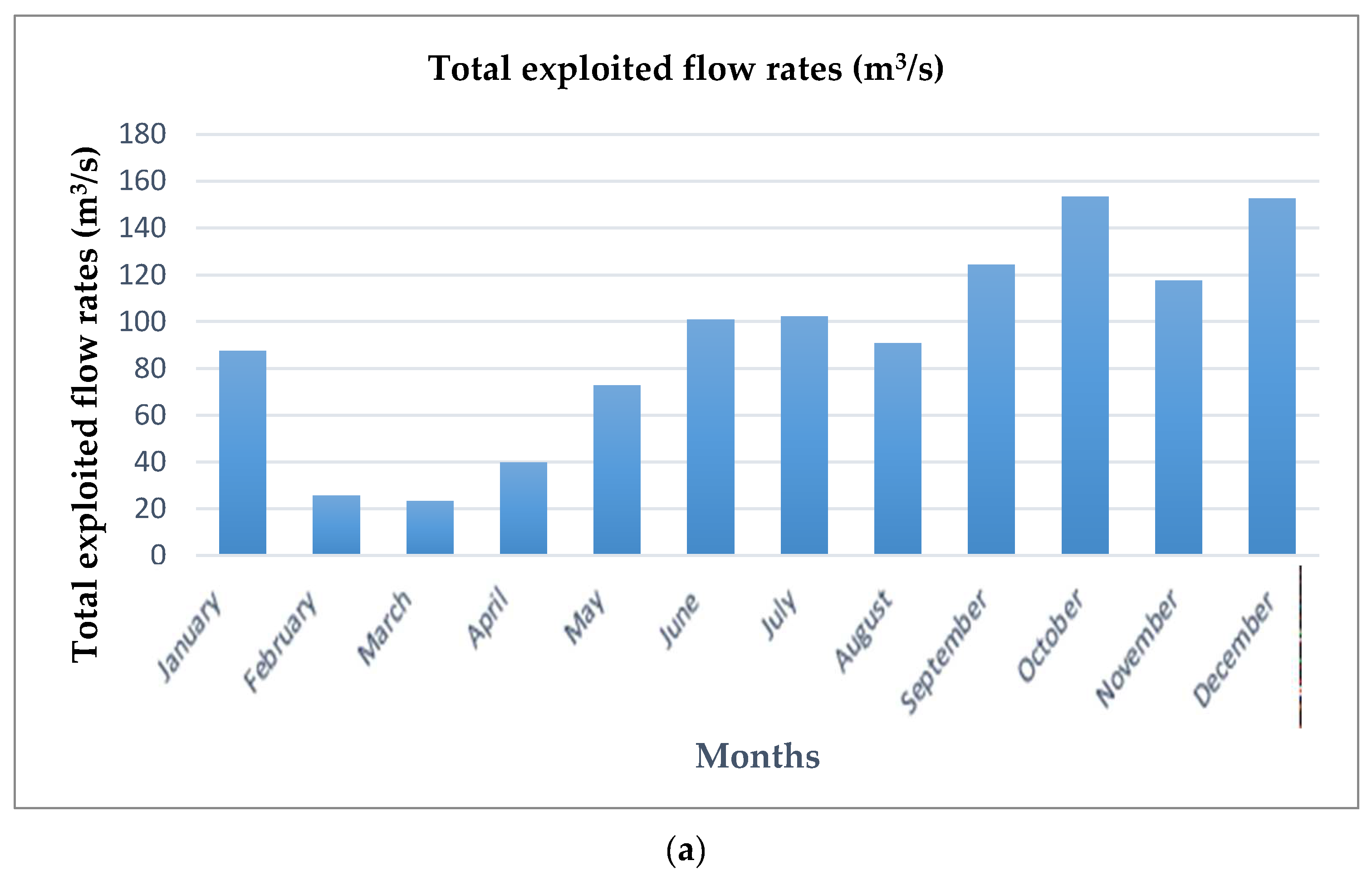
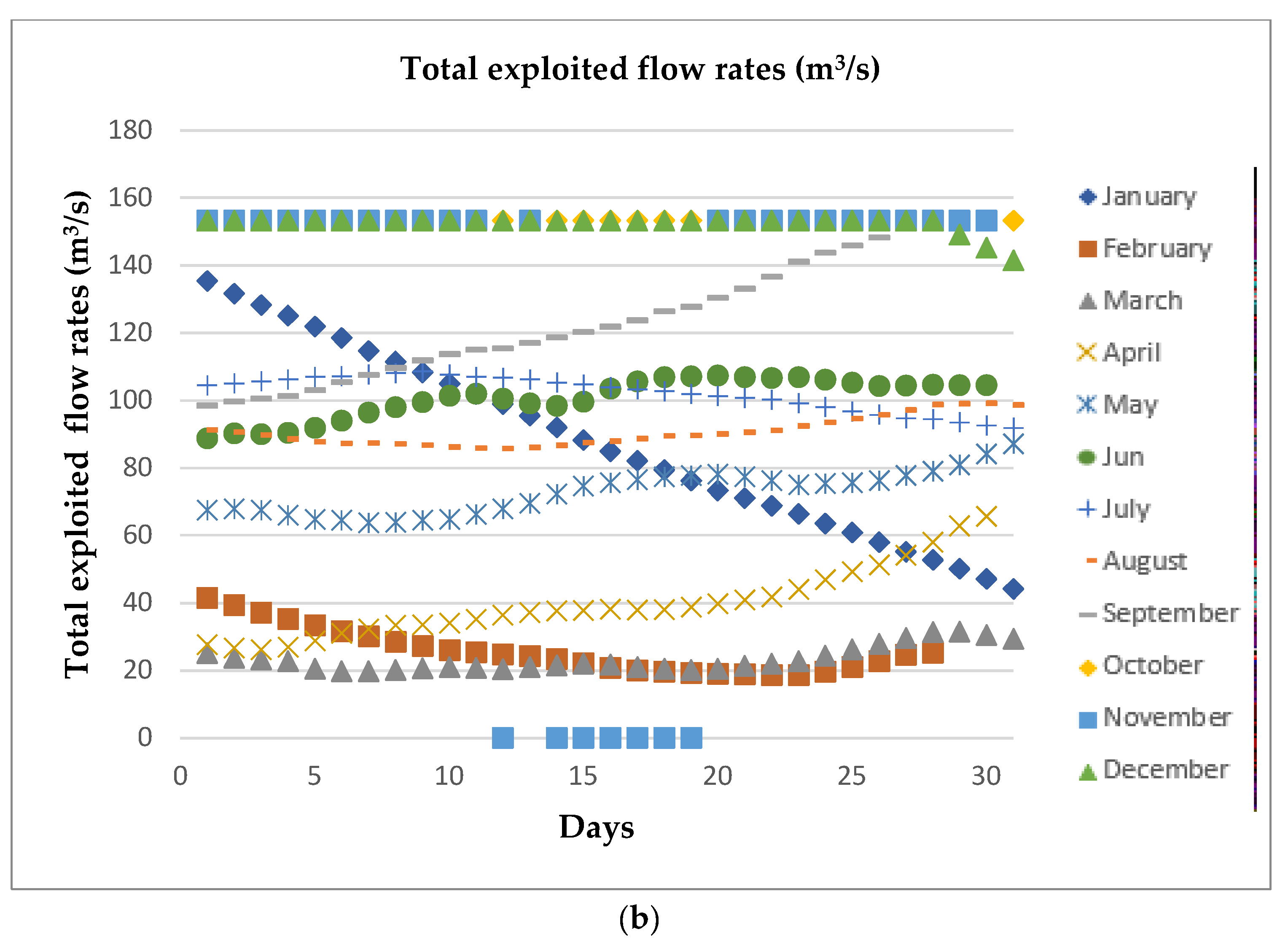
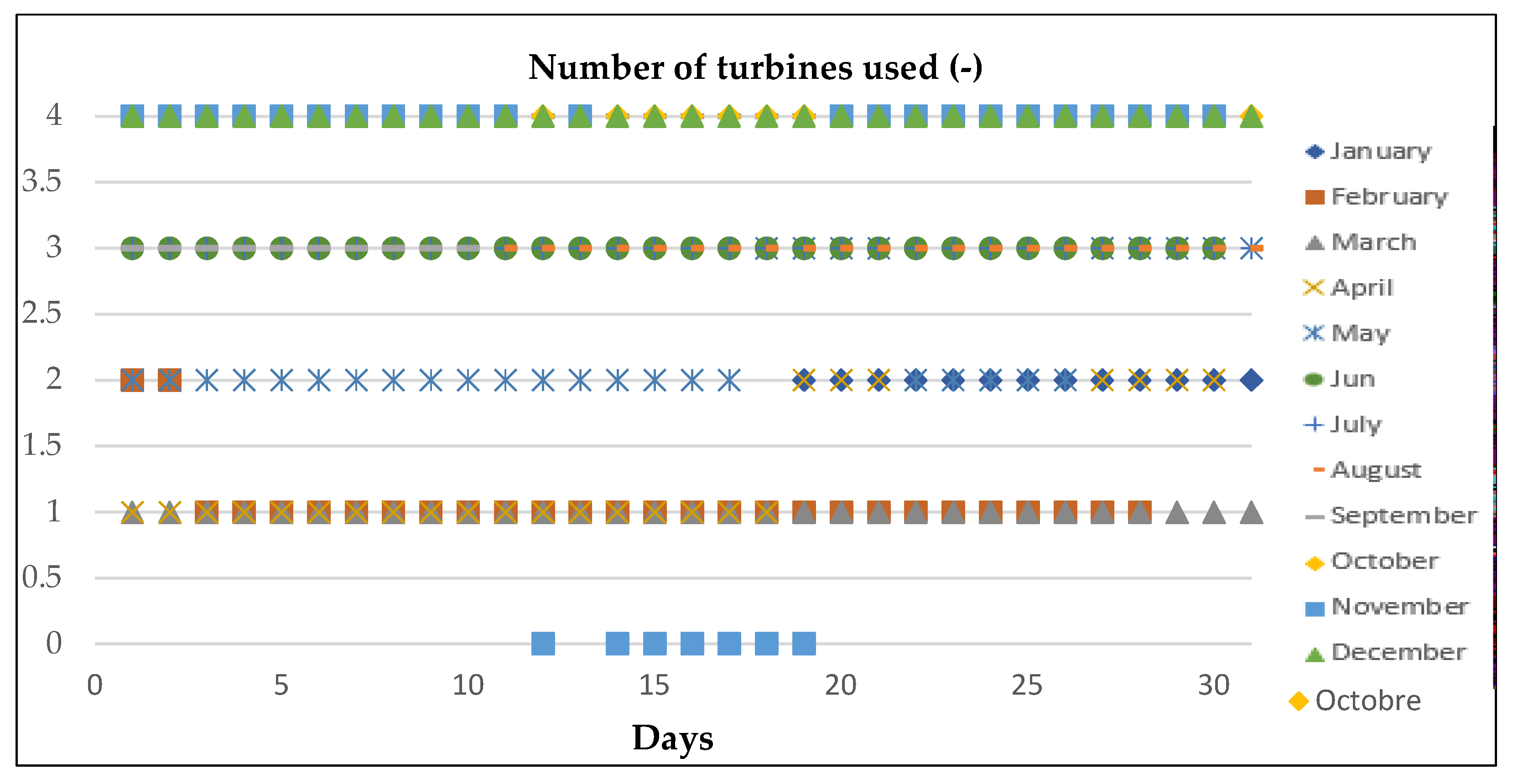
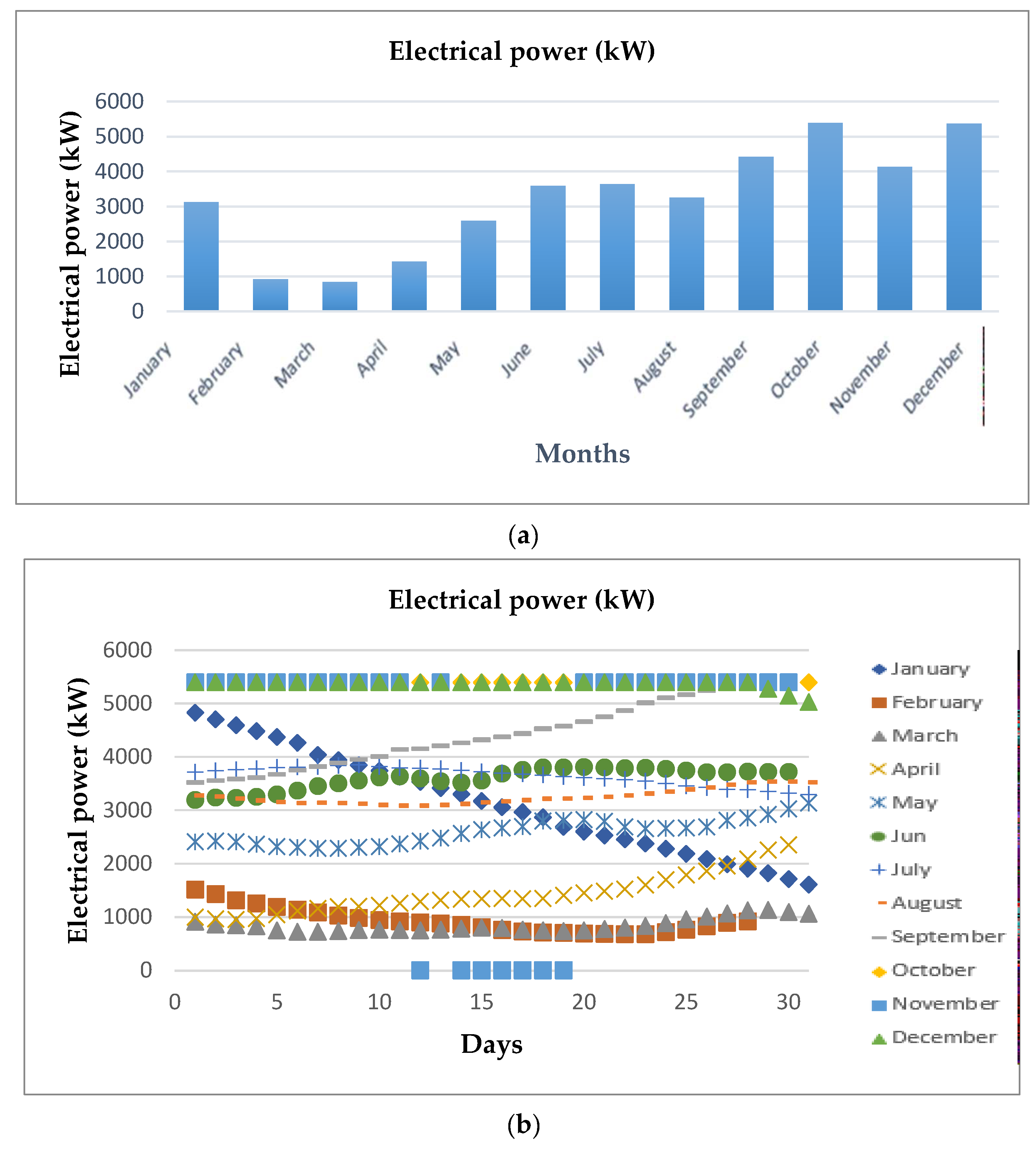
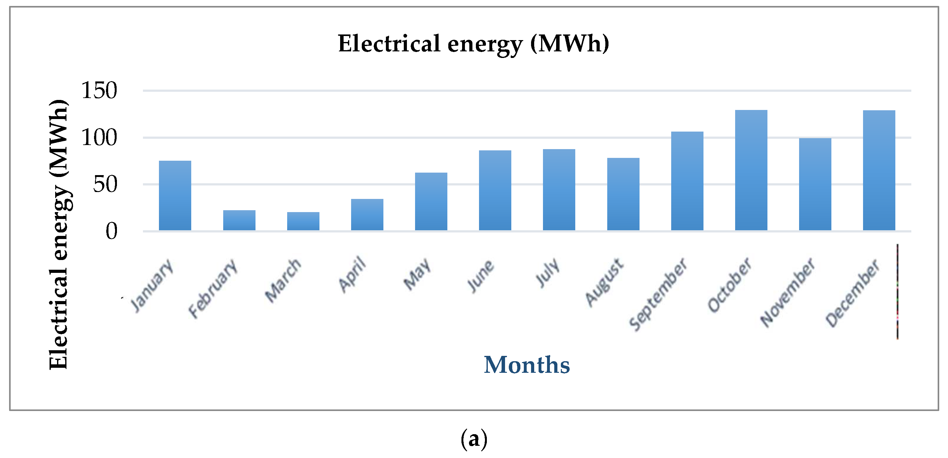
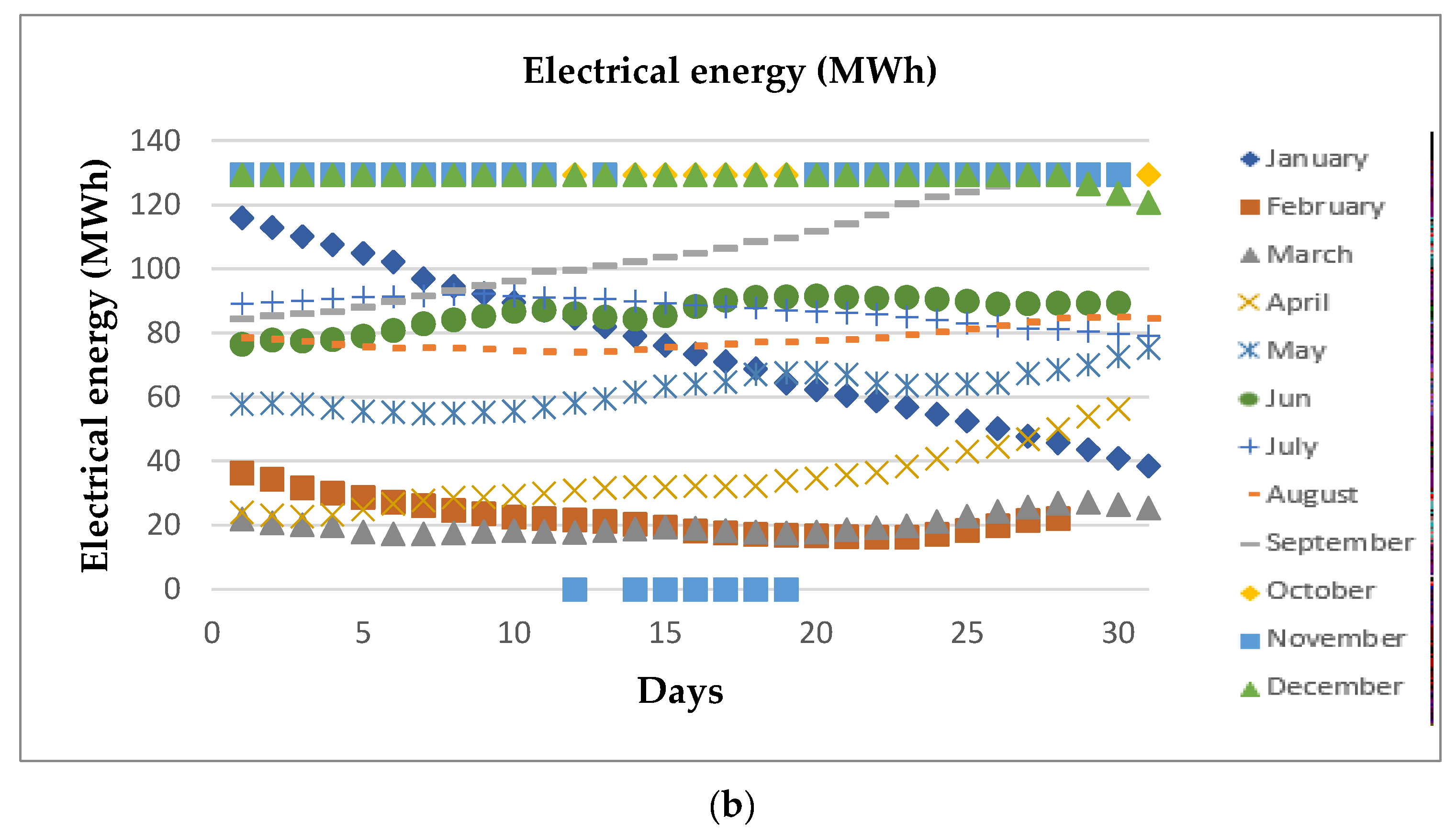
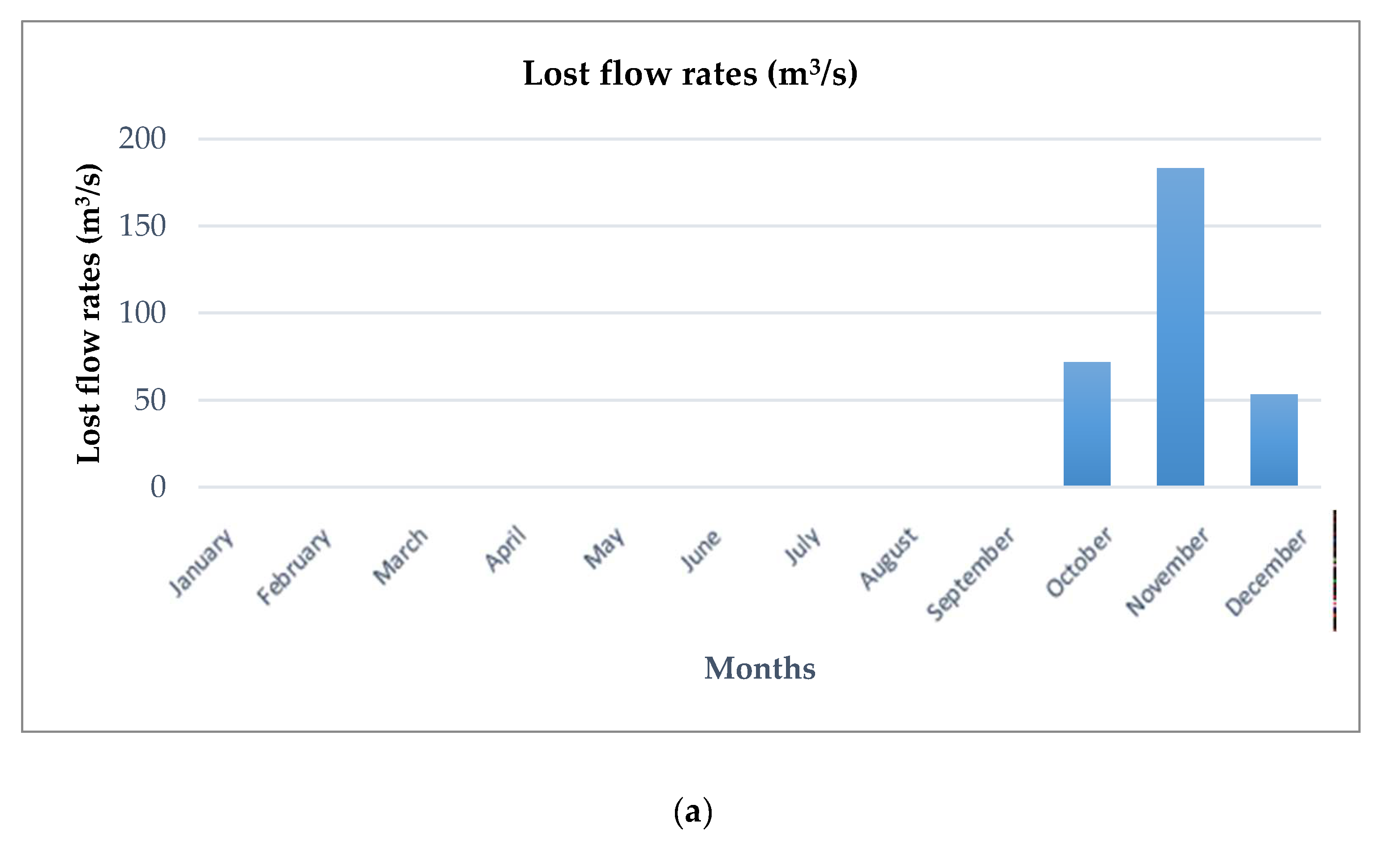
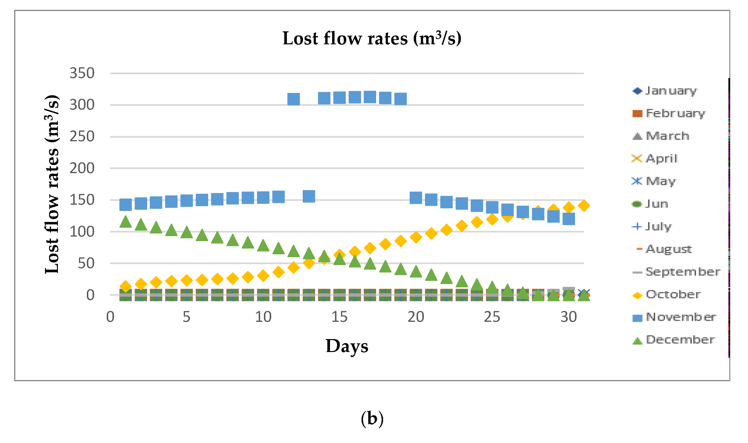
4.2. Optimal System Operation over the Year

Figure 8a,b show the flow rates that can be directly used by the power plant. That is to say, the flow rates remaining after subtracting from the available flow rates and the residual flow rate, which is the flow rate reserved for environmental reasons. As partially introduced, the exploitable flow rates during February to April are very low and almost always below 50 m³/s, thus making the exploitation of this watercourse particularly difficult during these months.

Figure 9 shows the exploited flow rates in the plant, which is to say the flows actually used. It can be seen in Figure 9b that only during the periods of November 13 and November 14 to 19 (only 7 days a year) the plant is shut down. The shutdown of the plant during these 7 days is due to the fact that the plant cannot exploit all the large flow rates in the month of November as, during these days, the daily exploitable flow rates, which are all greater than the safety flow rate (309.17 m³/s), is beyond which the safety of the plant is no longer guaranteed.

As for the other days of the year, the plant remains in operation by efficiently using the exploitable flow rates.

Therefore, the configuration proposed by the model makes it possible to not only to use large flow rates, of the order of the equipment flow rate when flow rates are strictly lower than the safety flow rate, but also to exploit very low flow rates such as those of the months of February, March, and April when the lowest exploitable flow rates of the year occur. With this configuration, the minimum and maximum flow rates that can be exploited by the power plant are 5.75 m³/s and 153.41 m³/s, respectively.

Figure 10 illustrates the optimal management of the system by showing the number of turbines that will operate each day of the year. Through this curve, it is noted that a maintenance schedule could be set up, thus reducing plant downtime, ensuring a more continuous production of electrical energy. In fact, according to the curve in Figure 10, for about 70% of the year, there are less than four turbines in operation in the plant.

Thus, as can be seen in Figure 11 and Figure 12, apart from the 7 days listed above, the plant is always in operation during the year, thus providing the grid with a large amount of electrical energy.

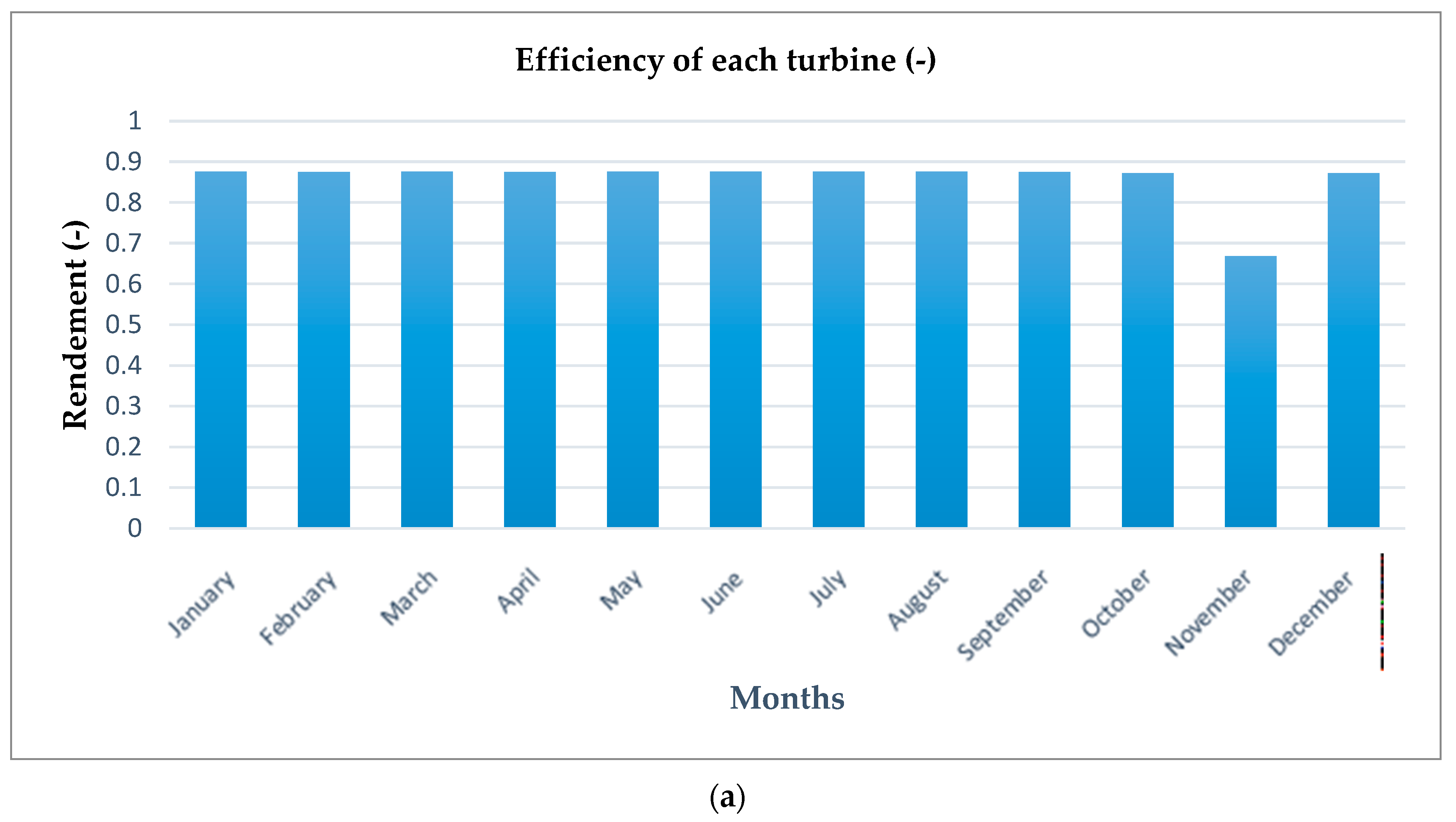
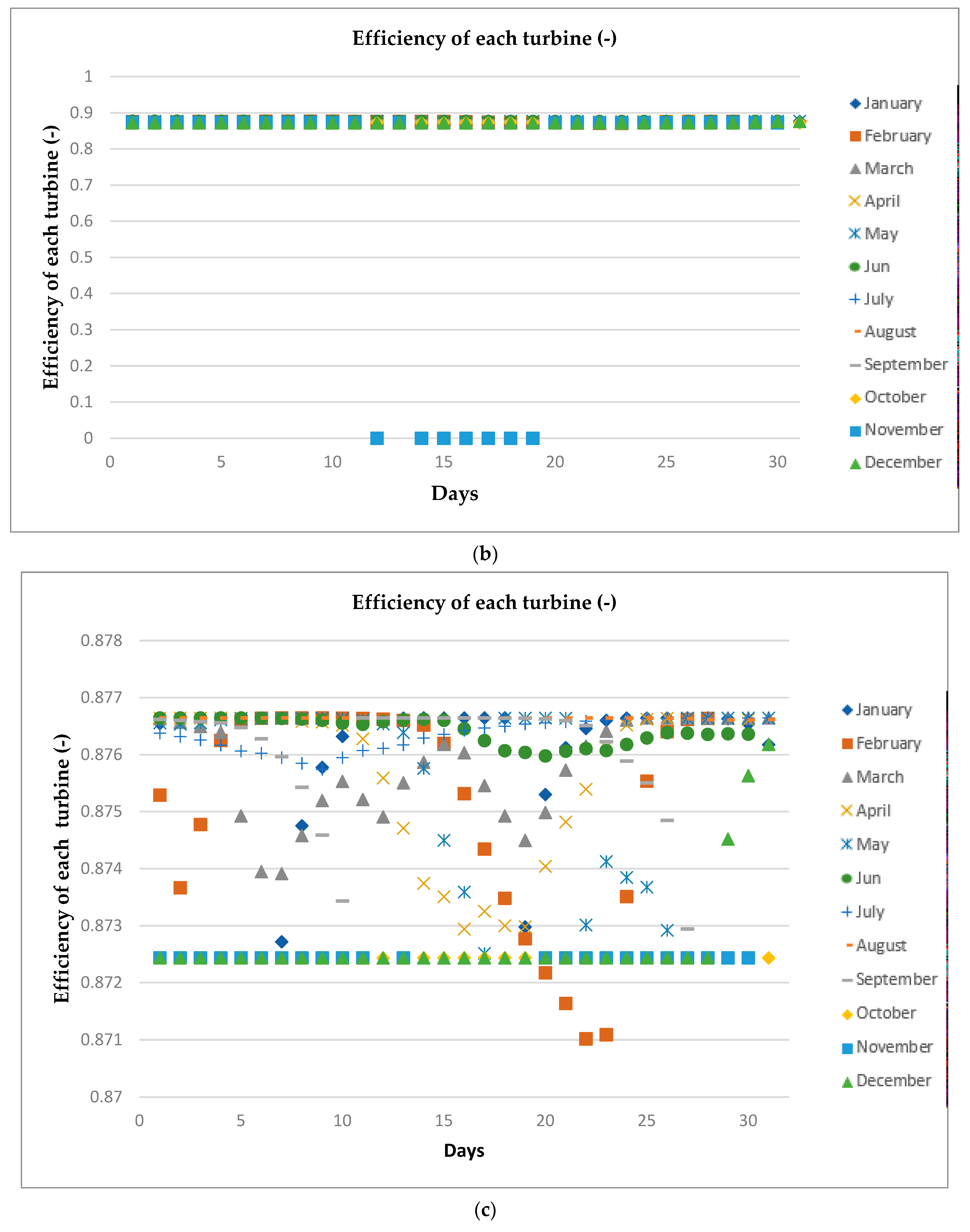
4.3. Analysis of the Energy Efficiency of the Optimal System

As shown again by the histogram and the curve in Figure 13, the exploitation of the hydraulic energy of the river Nyong, in Mbalmayo, is limited not only by the minimum and maximum operating flow rates of the turbines, but also by the safety flow rate beyond which the plant infrastructure could be damaged. November has the largest amount of flow rates that cannot be managed due to the danger they could represent for the plant. From 28 September to 27 December, for example, flow rates—hence hydraulic energy—decrease every day continuously either due to flow rates being higher than the maximum flow rates of the turbines, or due to the flow rates being greater than the safety flow rate. This is the case during the periods of the 13th and from 14 to 19 November, thus forcing the power plant to be shut down (here, all exploitable flow rates are lost). All the constraints presented above, therefore, prevents the exploitation of a total flow rate of 9386.41 m³/s per year (or hydraulic energy of about 11.05 GWh per year).

However, the histogram and the turbine efficiency curves in Figure 14 show that every time the plant is in operation, each turbine has an efficiency greater than or equal to 0.87.

We can also see through these results the interest of using several turbines in parallel to increase the energy efficiency of the plant. For example, let us pay attention to the period from 3 February to 18 April in which only one turbine is in operation. As such, if that plant were a single large turbine, the plant would have been shut down several times during these periods because, in some cases, exploitable flow rates would have been below the minimum starting flow rate of the large turbine. Another matter to emphasize is that even in cases where the flow rates would have been greater than the minimum starting flow rate of the large turbine, the large difference between these flow rates and the design flow rate of the large turbine (here equal to the equipment flow rate) would have brought the system to operate with very a poor performance or with low efficiency.

Anagnostopoulos and Papantonis [20] also suggested the use of three indices in order to assess the energy efficiency of a hydroelectric plant: the energy production index, obtained by dividing the total annual energy production by the total annual exploitable hydraulic energy; the water exploitation index, which is the fraction of the exploitable flow rates used; and the load index, which is the ratio of the average daily power produced over the year to the rated power of the plant. The values for the proposed case study are reported in

Table 14. Energy criteria.

Energy Criteria
Total installed capacity (MW)	6.32
Productible (GWh)	28.42
Water exploitation Index (%)	78.04
Energy production Index (%)	56.47
Average efficiency of the turbines over the year (-)	0.88
Load Index (%)	51.32

.

In general, the energy efficiency of the system is quite good, even if the values of certain energy criteria do not emphasize it sufficiently. The water exploitation index shows, for example, that the configuration proposed by our model exploits approximately 78.04% the available flow rates; the rest is lost due to the constraints linked due to not only to the maximum turbine operating flow rate, but also to the safety flow rate. The value of the energy production index is only 56.47% due to the large quantity of lost flow rates presented above and the head losses. The value of the load index is only 51.32% not only because there are periods during which the plant is shut down, but also because the plant uses its four turbines simultaneously only 111 days per year. During this period the plant operates at full capacity 85 days per year, due to the fact that on the rest of the days of the year either the exploitable flow rates are not high enough to trigger the startup of the four turbines, or they are greater than the safety flow rate.

4.4. Economic Analysis of the Optimal System

Table 15. Economic criteria.

Economic Criteria
LCC (MUSD)	11.37
LCOE (USD/kWh)	0.0502
Net Present Value (MUSD)	11.30
Payback period (years)	5 years 2 months
Cost of civil works (MUSD)	2.13
Cost of electromechanical equipment (MUSD)	3.13
Miscellaneous and indirect cost (MUSD)	1.09
Initial investment cost (MUSD)	5.94
Replacement cost over the lifetime project (MUSD)	3.54
Total investment cost over the lifetime project (MUSD)	9.48
Operation and Maintenance cost per year (MUSD)	0.237

details the different costs of the optimal run-of-river hydroelectric system proposed in this study. The minimum LCOE (0.05 USD/kWh) obtained here remains in the range (0.05–0.12 USD/kWh) as per

Table 16. General values of LCOE for hydropower projects [60].

No.	Investment Cost (IC) (USD2005/kW)	O&M Cost (% of IC)	Capacity Factor (%)	Lifetime (Years)	Discount Rate (%)	LCOE (cents/kWh)	Comments
1	˂500–6200 Median 1650 90% below 3250		41–61				2155 Projects in USA 43,000 MW in total Annual Capacity factor (except Rhode Island)
2	˂500–4500 Median 1000 90% below 1700		55–60				250 Projects for commissioning 2002–2020 Total Capacity 202,000 MW Worldwide but mostly Asia and Europe
3	1000–3500 700–8000		35–60 20–90			2–10 2–12	Large Hydro Small Hydro (˂10 MW) (Not explicitly stated as levelized cost in report)
4	2184	2.5	45	40	10	7.1
5	1000–5500 2500–7000	2.2–3			10 10	3–12 5.6–14	Large Hydro Small Hydro
6	2880 in 2010	4	45	40	10	10.4
7	2440				6	7.3	Study applies to Germany only
8	1000–5500	4	33	30		9.8	Indicative average LCOE year 2000
9	750–19,000 in 2010 (1278 average)		51	80 80		2.3–45.9 4.8	Range for 13 projects from 0.3 to 18,000 MW Weighted average for all projects
10						5–12 3–5 5–40	Small Hydro (˂10 MW) Large Hydro (˃10 MW) Off-Grid (˂1 MW)

of the LCOE for hydroelectric projects with a power of less than 10 MW as presented in the special report of the IPCC (Intergovernmental Panel on Climate Change) [60]. In the same way, according to IRENA [53], the small hydropower projects have an average LCOE of 0.05 USD/kWh. Therefore, the proposed configuration allows one to have robust LCOE estimations in alignment with other studies in the literature.

In addition, by taking an energy price of 0.1 USD/kWh (or about 55 F CFA/kWh), the payback period is about 5 years and 2 months for the project (assuming a lifetime of 50 years) with a Net Present Value of 11.3 MUSD (approximately 6.1 billion CFA Francs). As according to ESHA [42], a small hydro project should have a payback period of less than 7 years to be considered profitable; therefore, the proposed configuration makes the project sufficiently profitable.

5. Conclusions and Future Scope

The objective of this study is to provide a model for the optimal sizing and techno-economic optimization of a small run-of-river hydroelectric power plant connected to an existing electricity network. This work focuses on the optimal design of the diameter and thickness of the penstock; the selection and optimal location of a turbine; the estimation of the production of electrical energy; and the estimation of the costs of a small run-of-river hydroelectric power plant, without pondage, when connected to an existing electricity network.

The study applies the model on a case study of the river Nyong in Mbalmayo. The results show that the optimal system is energy efficient, with efficiency beyond 87%, and successfully converts about 78% of the exploitable flow rates of the stream into electricity; however, the flow rates fluctuate significantly, between 31.71 m³/s and 325.75 m³/s. Moreover, these results show that the proposed configuration is also very cost effective as its LCOE is around 0.05 USD/kWh (which is the lowest limit for the interval of LCOE for small hydropower plants as presented in the report of the IPCC). Its Net Present Value is USD 11.3 billion, or about 6.1 billion CFA Francs, assuming an energy price of 0.1 USD/kWh (or about 55 F CFA/ kWh), and its payback time is about 5 years 2 months—when it must be less than 7 years to be considered profitable according to ESHA— assuming a lifespan of 50 years.

This study is expected to provide a solid base for scholars and developers who are interested in developing preliminary feasibility studies for run-of-river hydropower plants in Sub-Saharan Africa, which are expected to be an important source of energy (especially for rural areas) with limited drawbacks. As for future works, it would be interesting to extend the analysis to estimate the hydropotential in the Central African context in order to propose a more reliable cost estimate model for small run-of-river hydroelectric plants. A second possible consideration for this work is to extend the analysis beyond a single hydropower plant, therefore combining multiple energy sources (e.g., a photovoltaic system) and/or a storage system, to meet the electrical energy needs of a population in isolated areas. In the end, the methodology developed in this study could lead to an optimal design tool for small hydro systems with a graphical user interface to ease its use by developers.

References

1. Safarian, S.; Unnborsson, R.; Ritcher, C. A review of biomass gasification modelling. Renew. Sustain. Energy Rev. 2019, 110, 378–391. [Google Scholar] [CrossRef]
2. Hydropower Status Report, Sector Trends and Insights 2019. Available online: www.hydropower.org (accessed on 15 March 2021).
3. Breeze, P. Power Generation Technologie; Elsevier: Amsterdam, The Netherlands, 2019. [Google Scholar]
4. Skoulikaris, C. Run-Of-River Small Hydropower Plants as Hydro-Resilience Assets against Climate change. Sustainability 2021, 13, 14001. [Google Scholar] [CrossRef]
5. Borkowski, D.; Cholewa, D.; Korzen, A. Run-of-the-River Hydro-PV Battery Hybrid System as an Energy Supplier for Local Loads. Energies 2021, 14, 5160. [Google Scholar] [CrossRef]
6. Kumar, D.; Katoch, S. Sustainability indicators for run of the river (RoR) hydropower projects in hydro rich regions of India. Renew. Sustain. Energy Rev. 2014, 35, 101–108. [Google Scholar] [CrossRef]
7. Goodland, R. Environmental sustainability and the power sector. Impact Assess. 2012, 12, 409–470. [Google Scholar] [CrossRef]
8. Korkovelos, A.; Mentis, D.; Siyal, H.; Arderne, C.; Rogner, H.; Bazilian, M.; Howells, M.; Beck, H.; Roo, D. A Geospatial Assessment of Small-Scale Hydropower Potential in Sub-Saharan Africa. Energies 2018, 11, 3100. [Google Scholar] [CrossRef] [Green Version]
9. Haddad, O.; Moradi-Jalal, M. Design–operation optimisation of run-of-river powerplants. Water Manag. 2011, 164, 463–475. [Google Scholar]
10. Vougioukli, A.; Didaskalou, E.; Georgakellos, D. Financial Appraisal of Small Hydro-Power Considering the Cradle-to-Grave Environmental Cost: A Case from Greece. Energies 2017, 10, 430. [Google Scholar] [CrossRef] [Green Version]
11. Okot, D. Review of small hydropower technology. Renew. Sustain. Energy Rev. 2013, 26, 515–520. [Google Scholar] [CrossRef]
12. Paish, O. Small hydro power: Technology and current status. Renew. Sustain. Energy Rev. 2002, 6, 537–556. [Google Scholar] [CrossRef]
13. Karlis, D.; Papadopoulos, P. A systematic assessment of the technical feasibility and economic viability of small hydroelectric system installations. Renew. Energy 2000, 20, 253–262. [Google Scholar] [CrossRef]
14. ONUDI Rapport Mondial sur le Développement de la Petite Hydraulique 2019. Available online: www.unido.org (accessed on 1 October 2021).
15. Jasper, A.; Veysel, Y. A toolbox for the optimal design of run-of-river hydropower plants. Environ. Model. Softw. 2019, 111, 134–152. [Google Scholar]
16. Tsuanyo, D.; Azoumah, Y.; Aussel, D.; Neveu, P. Modeling and optimization of batteryless hybrid PV (photovoltaic)/Diesel systems for off-grid applications. Energy 2015, 86, 152–163. [Google Scholar] [CrossRef]
17. Tapia, C.; Gutiérrez, R.; Millan, G. An Evolutionary Computational Approach for Designing Micro Hydro Power Plants. Energies 2019, 12, 878. [Google Scholar] [CrossRef] [Green Version]
18. Panagiotis, I.; Konstantinos, L. Optimizing Current and Future Hydroelectric Energy Production and Water Uses of Complex Multi-Reservoir System in the Aliakmon River, Greece. Energies 2020, 13, 6499. [Google Scholar]
19. Anagnostopoulos, J.; Papantonis, D. Application of evolutionary algorithms for the optimal design of a small hydroelectric power plant. In Proceedings of the HYDRO 2004: A New Era for Hydropower, Porto, Portugal, 18–21 October 2004; Available online: www.researchgate.net (accessed on 10 March 2021).
20. Anagnostopoulos, J.; Papantonis, D. Optimal sizing of a run-of-river small hydropower plant. Energy Convers. Manag. 2007, 48, 2663–2670. [Google Scholar] [CrossRef]
21. Getachew, E.; Miroslav, M.; Juan, C.; Franca, J. Optimization of Run-of-River Hydropower Plant Capacity. Water Power Dam Constr. 2018, 1–10. Available online: www.researchgate.net (accessed on 22 March 2020).
22. Ibrahim, M.; Imam, Y.; Ghanem, A. Optimal Planning and Design of Run-of-river Hydroelectric Power Projects. Renew. Energy 2019, 141, 858–873. [Google Scholar] [CrossRef]
23. Kumar, A.; Singhal, M. Optimum Design of Penstock for Hydro Projects. Int. J. Energy Power Eng. 2015, 4, 216–226. [Google Scholar]
24. Chinyere, A.; Obasih, R.; Ojo, E.; Okonkwo, C.; Mafiana, E. Technical Details for the Design of a Penstock for Kuchigoro Small Hydro Project. Am. J. Renew. Sustain. Energy 2017, 3, 27–35. [Google Scholar]
25. Alexander, K.; Giddens, E. Optimum penstocks for low head microhydro schemes. Renew. Energy 2008, 33, 507–519. [Google Scholar] [CrossRef]
26. Voros, N.; Kiranousdis, C.; Maroulis, Z. Short-cut design of small hydroelectric plants. Renew. Energy 2000, 19, 545–563. [Google Scholar] [CrossRef]
27. Munir, M.; Shakir, A.; Khan, M. Optimal Sizing of Low Head Hydropower Plant- A Case Study of Hydropower Project at Head of UCC (Lower) at Bambanwala. Pak. J. Engg. Appl. Sci. 2015, 16, 73–83. [Google Scholar]
28. Adejumobi, I.; Shobayo, D. Optimal selection of hydraulic turbines for small hydroelectric power generation—A case study of Opeki river, South Western Nigeria. Niger. J. Technol. 2015, 34, 530–537. [Google Scholar] [CrossRef]
29. Sangal, S.; Garg, A.; Kumar, D. Review of Optimal Selection of Turbines for Hydroelectric Projects. Int. J. Emerg. Technol. Adv. Eng. 2013, 3, 424–430. [Google Scholar]
30. Mishra, S.; Singal, K.; Khatod, D. A review on electromechanical equipment applicable to small hydropower plants. Int. J. Energy Res. 2012, 5, 553–571. [Google Scholar] [CrossRef]
31. Mishra, S.; Singal, K.; Khatod, D. Approach for Cost Determination of Electro-Mechanical Equipment in RoR Projects. Smart Grid Renew. Energy 2011, 2, 63–67. [Google Scholar] [CrossRef] [Green Version]
32. Mishra, S.; Singal, K.; Khatod, D. Cost Optimization of High Head Run of River Small Hydropower Projects. In Application of Geographical Information Systems and Soft Compuation Techniques in Water and Water Based Renewable Energy Problems; Springer: Singapore, 2018; pp. 141–166. [Google Scholar] [CrossRef]
33. Singal, K.; Saini, P.; Raghuvanshi, S. Analysis for cost estimation of low head run-of-river small hydropower schemes. Energy Sustain. Dev. 2010, 14, 117–126. [Google Scholar] [CrossRef]
34. Ogayar, B.; Vidal, P. Cost determination of the electro-mechanical equipment of a small hydro-power plant. Renew. Energy 2009, 34, 6–13. [Google Scholar] [CrossRef]
35. Singal, K.; Saini, P.; Raghuvanshi, S. Cost Optimisation Based on Electro-Mechanical Equipment of Canal Based Low Head Small Hydropower Scheme. Open Renew. Energy J. 2008, 1, 26–35. [Google Scholar]
36. Singal, K.; Saini, P. Analytical Approach for Cost Estimation of Low Head Small Hydropower Schemes. In Proceedings of the International Conference on Small Hydropower-Hydro Sri Lanka, New Delhi, India, 22–24 October 2007. [Google Scholar]
37. Aggidis, G.; Luchinskaya, E.; Rothschild, R.; Howard, D. The costs of small-scale hydro power production: Impact on the development of existing potential. Renew. Energy 2010, 35, 2632–2638. [Google Scholar] [CrossRef]
38. Najmaii, M.; Movaghar, A. Optimal Design of Run-of-River Power Plants. Water Resour. Res. 1992, 28, 991–997. [Google Scholar] [CrossRef]
39. Santolin, A.; Gavazzini, G.; Pavesi, G.; Rossetti, A. Techno-economical method for the capacity sizing of a small hydropower plant. Energy Convers. Manag. 2011, 52, 2533–2541. [Google Scholar] [CrossRef]
40. Patro, E.; Kishore, T.; Haghighi, A. Levelized Cost of Electricity Generation by Small Hydropower Projects under Clean Development Mechanism in India. Energies 2022, 15, 1473. [Google Scholar] [CrossRef]
41. ESHA Guide on How to Develop a Small Hydropower Plant. 2004. Available online: www.canyonhydro.org (accessed on 17 March 2019).
42. Pigueron, Y.; Dubas, M. Guide pour l’étude sommaire de petites centrales hydrauliques, Hes.so 2009. Available online: www.vs.ch (accessed on 17 March 2019).
43. Martin, J.; Tchouate, H. La Filière Hydroélectrique: Aspects Technologiques et Environnementaux; Université Catholique de Louvain-GEB: Louvain, Belgique, 2003. [Google Scholar]
44. Hänggi, P.; Weingartner, R. Variations in discharge volumes for hydropower generation in Switzerland. Water Resour. Manag. 2012, 26, 1231–1252. [Google Scholar] [CrossRef] [Green Version]
45. Ye, L.; Ding, W.; Zeng, X.; Xin, Z.; Wu, J.; Zhang, C. Inherent Relationship between Flow Duration Curves at Different Time Scales: A Perspective on Monthly Flow Data Utilization in Daily Flow Duration Curve Estimation. Water 2018, 10, 1008. [Google Scholar] [CrossRef] [Green Version]
46. Chen, J.; Yang, H.; Liu, C.; Lau, C.; Lo, M. A novel vertical axis water turbine for power generation from water pipelines. Energy 2013, 54, 184–193. [Google Scholar] [CrossRef]
47. Ramos, H. Guidelines for Design of Small Hydropower Plants, Belfast, North Ireland. WREAN (West. Reg. Energy Agency Netw.) DED (Dep. Econ. Dev.). 2000. Available online: www.civil.ist.utl.pt (accessed on 18 March 2020).
48. Parish, O.; Fraenkel, P.; Bokalders, V. Micro-Hydro Power A Guide for Development Workers; Practical Action Publishing: Rugby, UK, 1991. [Google Scholar]
49. Jantasuto, O. Review of small hydropower system. Int. J. Adv. Cult. Technol. 2015, 3, 101–112. [Google Scholar] [CrossRef]
50. RetScreen International Clean Energy Project Analysis, 2001–2004. Available online: www.ieahydro.org (accessed on 17 March 2019).
51. Kishore, T.S.; Patro, E.R.; Harish, V.S.K.V.; Haghighi, A.T. A Comprehensive Study on the Recent Progress and Trends in Development of Small Hydropower Projects. Energies 2021, 14, 2882. [Google Scholar] [CrossRef]
52. Tsuanyo, D.; Approches Technico-Economiques D’optimisation des Systèmes Energétiques Décentralisés: Cas des Systèmes Hybrides PV/Diesel. Ph.D. Thesis, Universite de Perpignan via Domitia, 2015. Available online: www.theses.fr (accessed on 15 April 2020).
53. Irena Renewable Power Generation Costs in 2014. Available online: www.irena.org (accessed on 25 October 2020).
54. Audry, S. Hydrological Data, Nyong, Cameroon [Data set]. Theia. 2012. Available online: https://mtropics.obs-mip.fr/products/?uuid=5dc044eb-b8a6-bce2-0e88-e3e97ec0ac87 (accessed on 2 October 2021).
55. Available online: www.infociments.fr (accessed on 2 October 2021).
56. Available online: www.4.ac-nancy-metz.fr (accessed on 2 October 2021).
57. The World’s Trusted Currency Authority. Available online: www.xe.com (accessed on 2 October 2021).
58. Kengne, S.; Hamandjoda, O.; Nganhou, J. Methodology of Feasibility Studies of Micro-Hydro power plants in Cameroon: Case of the Micro-hydro of KEMKEN. Energy Procedia 2017, 119, 17–28. [Google Scholar] [CrossRef]
59. Available online: www.process.free.fr (accessed on 2 October 2021).
60. Ahenkorah, A.; Caceres, R. Jean-Michel Hydropower. In IPCC Special Report on Renewable Energy Sources and Climate Change Mitigation; Cambridge University Press: Cambridge, UK; New York, NY, USA, 2011. [Google Scholar]
Figure 1. Site configuration of the model.
Energies 15 07507 g001
Figure 2. Turbine application chart [46].
Energies 15 07507 g002
Figure 3. Cross section of a Francis runner.
Energies 15 07507 g003
Figure 4. Cross section of a Kaplan turbine.
Energies 15 07507 g004
Figure 5. Schematic plant layout and parameters for optimization.
Energies 15 07507 g005
Figure 6. Optimization process minimizing LCOE.
Energies 15 07507 g006
Figure 7. (a) Average monthly available flow rates histogram, (b) average daily available flow rates curve, and (c) flow duration curve of the river Nyong (1998–2013).
Energies 15 07507 g007
Figure 8. (a) Average monthly exploitable flow rates histogram and (b) average daily exploitable flow rates curve.
Energies 15 07507 g008
Figure 9. (a) Average monthly exploited flow rates histogram and (b) average daily exploited flow rates curve.
Energies 15 07507 g009aEnergies 15 07507 g009b
Figure 10. Curve of the number of turbines used.
Energies 15 07507 g010
Figure 11. (a) Average monthly electrical power histogram and (b) average daily electrical power curve.
Energies 15 07507 g011
Figure 12. (a) Average monthly electrical energy histogram and (b) average daily electrical energy curve.
Energies 15 07507 g012aEnergies 15 07507 g012b
Figure 13. (a) Average monthly lost flow rates histogram and (b) average daily lost flow rates curve.
Energies 15 07507 g013aEnergies 15 07507 g013b
Figure 14. (a) Average monthly turbine efficiency histogram and (b,c) average daily turbine efficiency curve.
Energies 15 07507 g014aEnergies 15 07507 g014b