Shape Optimization of Oscillating Buoy Wave Energy Converter Based on the Mean Annual Power Prediction Model

Abstract

In order to improve the energy capture efficiency of an oscillating buoy wave energy converter (WEC), a buoy-shape optimization design method based on the mean annual power prediction model is proposed. According to the statistical data of long-term wave characteristics in the Chinese sea area, the optimal design space is determined. Sixty-three sample points were randomly selected in the optimized space. Based on simulation, the mean annual power corresponding to each sample point is calculated to quantitatively describe the energy capture ability. The response surface method (RSM), radial basis function neural network (RBFNN), and elliptical basis functions neural network (EBFNN) are used to establish the mean annual power prediction models, respectively. By combining the prediction model with the multi-island genetic algorithm (MIGA), the optimal solution in the design space is easily obtained. The reliability of the optimal solution is further proved by quantitative analysis about the influence of optimization parameters on the mean annual captured power. Compared with the common RSM and RBFNN methods, the prediction model established by the EBFNN method has a higher prediction accuracy. In the optimization process, the simulation calculation is replaced by a prediction model, which can effectively solve the problem of high simulation calculation cost.

1. Introduction

In recent years, the energy crisis and environmental problems have become increasingly serious. Vigorously developing and utilizing renewable energy has become a universal consensus of the international community [1,2]. Wave energy is a kind of clean and renewable energy. The theoretical reserve of the global wave energy resource is 3 TW, and further development can effectively alleviate the pressure of the global energy shortage [3]. Therefore, various wave energy converters (WECs) have been developed after decades of research and exploration. The WEC has gradually developed from the original concept of various and different types into five of the most typical device forms, namely, oscillating, raft, wave crossing, pendulum and oscillating water column [4,5,6]. The oscillating WEC has the characteristics of a simple structure, high power generation efficiency, and is not limited by water depth. It has received extensive attention, and many prototypes of oscillating WECs have been developed, such as the Archimedes Wave Swing, Power Buoy, Aqua Buoy, and Wavebob [7,8,9,10].

However, these prototypes have not been implemented into commercial operation, because of the low power generation efficiency and poor stability of WECs. In order to achieve the goal of high efficiency and stable output, researchers have carried out a lot of work, such as buoy optimization, power take-off (PTO) improvement, control strategy, and so on. Optimizing the buoy shape is one of the important ways to improve the wave power generation efficiency [11]. Therefore, many scholars have carried out related research. Some scholars have studied the hydrodynamic characteristics of the oscillating buoy, and analyzed the influence of buoy-shape parameters on energy capture efficiency to optimize the buoy shape. In order to efficiently extract the energy, Goggins et al. [12] established the optimal structural geometry and analyzed the optimal configuration for devices with a different radius. Shi et al. [13] numerically simulated the heave motion of conical bottom buoys with different masses and cross-sectional surfaces, and analyzed the effects of mass and cross-sectional surfaces on the energy capture. In order to analyze the effect of shape change on wave energy capture efficiency, Berenjkoob et al. [14] constructed 10 different geometric models under the same conditions. The results show that the proper shape was more efficient in capturing wave energy. Shadman et al. [15] took the cylindrical buoy as the research object and used the design of experiments (DOE) method to optimize the design parameters. Under the condition of mooring, Wu [16] obtained the optimal design parameters of the buoy by limiting the maximum displacement of the buoy and changing the draft ratio of the buoy radius. Some scholars also have used the heuristic algorithm to optimize buoy shape, such as genetic algorithm (GA), particle swarm optimization (PSO) et al. McCabe et al. [17] used a B-spline surface to parameterize the buoy geometry, and automatically optimized shapes based on GA. After 50,436 simulation calculations, a better design scheme was obtained. Garcia-Teruel et al. [18] further analyzed the adaptation of different algorithms such as GA and PSO, and used the non-dominated sorting genetic algorithm (NSGA-II) algorithm for multi-objective optimization design. Neshat et al. [19] optimized buoy shape and PTO based on bio-inspired swarm-evolutionary optimization algorithms. In general, the optimal buoy is mainly attained by analyzing the response relationship between the buoy parameters and the captured power, or by searching the design space through the heuristic optimization algorithm. Whether analyzing the response relationship or searching in the design space, enough sampling points are required. The hydrodynamic parameters of each sampling point are obtained by simulation to calculate the buoy captured power. Obviously, the hydrodynamic calculations take the majority of time during the buoy optimization. The significant time cost is considered a challenge for engineering design.

Therefore, reducing the simulation calculation times can effectively improve the optimization efficiency and reduce the optimization time cost. The prediction model is one of the best choices because it requires only a small number of simulation calculations. Prediction models have been used to solve the WEC optimization problems in engineering design and have been proven to be useful. Ji et al. [20] applied the response surface method (RSM) to build a hydrodynamic coefficients prediction model, which was used to calculate the captured power. Koh et al. [21] used the RSM prediction model to replace the simulation calculation, which determined the WEC geometric parameters. Colby et al. [22] developed a neural network function approximator and combined it with an evolutionary algorithm to optimize the WEC ballast configuration. The power output was maximized under a specific wave climate. Avila et al. [23] have predicted the energy generated from different WECs in the Canary Islands by using the Monte Carlo method. Avila et al. [24] proposed two mathematical models to forecast the wave energy based on fuzzy inference systems (FIS) and artificial neural networks (ANN), respectively. Wang et al. [25] proposed a prediction model of WEC buoy energy absorption power based on a back-propagation neural network (BPNN). Liu et al. [26] trained a radial basis function neural network (RBFNN) prediction model, which took the combination of design parameters as input and the capture factor as output. The prediction model was used with the genetic algorithm to optimize the converters, and the high-performance converter was obtained. Commonly, the prediction model indicates the mapping relations between the input (e.g., design parameter combinations of the buoy) and the output (e.g., capture factors, capture power, etc.), which is established by means of mathematical models. Combining the prediction model with the optimization algorithm to find the optimal solution in the design space becomes an optimization method that can quickly obtain the optimization results. So the accuracy of the prediction model is directly related to the reliability of the optimization results.

In recent years, methods such as RSM, BPNN, and RBFNN have been applied to WECs optimization design, but there are some shortcomings. The RSM cannot guarantee that the response surface passes through all the sample points, and the prediction effect of the highly complex functional relationship is not as good as that of the RBFNN. The BPNN has a slow convergence speed and might fall into local optimal solutions. The RBFNN has strong fault tolerance, but the modeling time is much longer than the RSM. Compared with the above methods, the elliptical basis functions neural network (EBFNN) has the advantages of a fast training speed and high prediction accuracy. Therefore, in order to improve the optimization efficiency, this paper proposes a mean annual power prediction model based on EBFNN. Compared with RSM and RBFNN, this method can establish a more accurate prediction model. Combining the mean annual power prediction model with MIGA can effectively reduce the simulation calculation time and improve the optimization design efficiency that an oscillating buoy with high performance can be easily designed. In this study, the optimization method not only optimizes the oscillating buoy, but also has the potential to solve other types of WECs optimization problems.

The remainder of this paper is organized as follows. Section 2 introduces the optimization method, including the geometric model, mathematical models, and optimization procedures. Section 3 is based on the wave statistics of the ocean near Chengshantou, Weihai City, Shandong Province, China; the mean annual power of the sample points is calculated. The prediction models with optimized parameters as input and mean annual power as output are established, respectively, by using RSM, RBFNN and EBFNN. Section 4 introduces the optimization results and discussion. Section 5 presents the conclusions.

2. Methodology

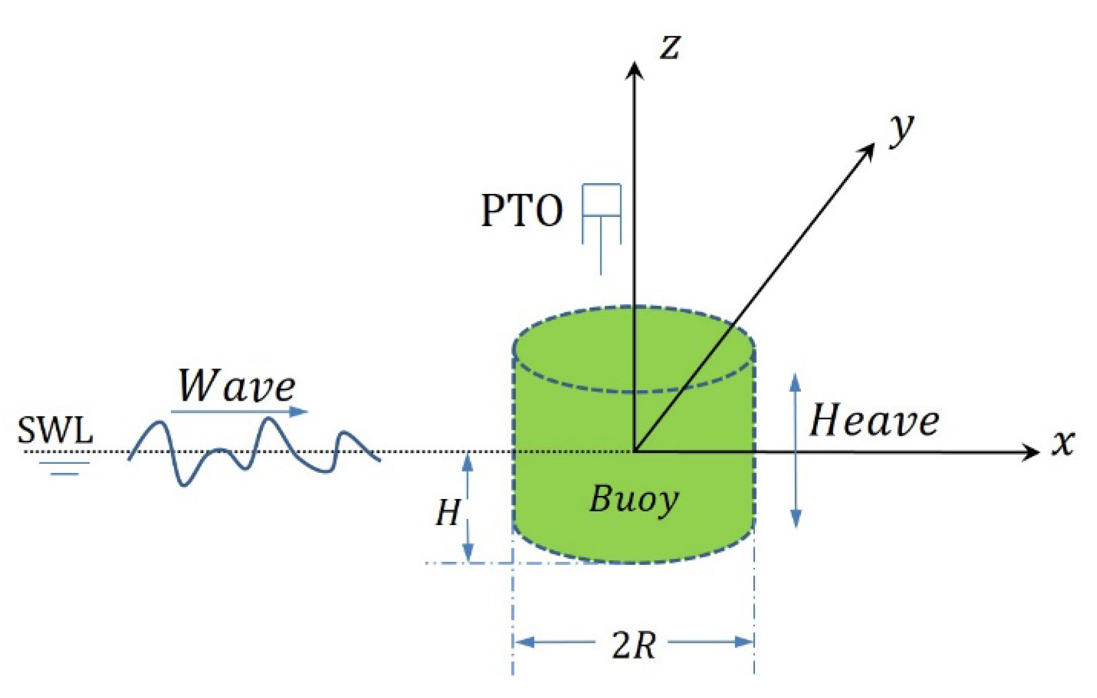
2.1. Geometric Model

The schematic diagram of the oscillating buoy WEC is shown in Figure 1. In this study, a generalized WEC is considered, which is a single buoy with an ideal linear damper as the PTO system. The buoy only does heave motion under wave excitation. In the case of slack mooring, the mooring force has little effect on the wave energy capture by the buoy [20,21]. Therefore, this paper ignores the mooring force acting on the buoy. The origin of the Cartesian coordinate system is at the calm waterline. The x-axis points to the direction of wave propagation. The z-axis passes vertically upward through the center of gravity of the buoy. The y-axis is perpendicular to the former according to the right-hand rule.

2.2. Mean Annual Power

The modified Pierson–Moskowitz (P–M) spectrum is used to describe the distribution of wave energy relative to each component wave [27]. The spectrum can be expressed as:

$$S_{\eta }\left(\omega \right)=\frac{173H_s^2{T}_{av}^{-4}}{{\omega }^5}\exp \left(-691T_{av}^{-4}{\omega }^{-4}\right)$$

(1)

where $H_s$ is the significant wave height, $T_{av}$ is the average wave period, $\omega$ is the wave angular frequency.

Divide the wave spectrum into 200 parts, the frequency ${\omega }_i$ is from 0.02 to 4 rad/s, then the frequency interval is 0.02 rad/s [28]. The energy per unit area of an irregular wave is given by:

$$\mathrm{E}=\mathsf{\rho }\mathrm{g}{\displaystyle \sum }_{i=1}^N{S}_{\eta }\left({\omega }_i\right)\Delta {\omega }_i=\frac{1}{2}\mathsf{\rho }\mathrm{g}{\displaystyle \sum }_{i=1}^N\alpha {\left({\omega }_i\right)}^2$$

(2)

where $\mathsf{\rho }$ is the density of the fluid, $\mathrm{g}$ is the acceleration due to gravity, $\Delta {\omega }_i$ is the frequency interval, $N$ is the number of component angular frequencies (200), and $\alpha \left({\omega }_i\right)$ are the component wave amplitudes. Hence, the component wave amplitudes can be expressed as:

$$\alpha \left({\omega }_i\right)=\sqrt{2S_{\eta }\left({\omega }_i\right)\Delta {\omega }_i}$$

(3)

Each sea state is assigned a set of proprietary random number generator seeds, from which repeatable normal distribution phase sets can be generated. The wave surface function of the i-th regular wave can be expressed as:

$${\eta }_{i,j}\left(t\right)=\alpha \left({\omega }_i\right)cos\left({\omega }_{i}t+{\epsilon }_{i,j}\right) j=1,2,\cdots ,10$$

(4)

where ${\epsilon }_{i,j}$ is the initial phase uniformly random distributed between 0 and 2 π, and is associated with angular frequency ${\omega }_i$. $j$ is the number of sea states. The corresponding incident wave is then synthesized by the linear superposition of all frequency components, as:

$${\eta }_j\left(t\right)={\displaystyle \sum }_{i=1}^N{\eta }_{i,j}\left(t\right)$$

(5)

Assuming an irrotational, non-viscous, and incompressible flow in the fluid domain, the waves are of small amplitude. Potential flow theory and three-dimensional radiation/diffraction theory are applied in the analysis. The velocity potential of the flow motion can be expressed as:

$$\varphi =\left(\overrightarrow{X},t\right)=\phi \left(\overrightarrow{X}\right)e^{-i\omega t}$$

(6)

where $t$ is the time, $\phi \left(\overrightarrow{X}\right)$ is the spatial velocity potential function, $\omega$ is the wave frequency.

$$\phi \left(\overrightarrow{X}\right)={\phi }_I+{\phi }_D+{\displaystyle \sum }_{j=1}^6{\phi }_{rj}{x}_j$$

(7)

where ${\phi }_I$ is the incident wave potential, ${\phi }_D$ is the diffracted wave potential, ${\phi }_{rj}$ is the radiation wave potential. $\phi \left(\overrightarrow{X}\right)$ satisfies the Laplace equation that can be expressed as:

$${\nabla }^2\mathsf{\phi }=0$$

(8)

The radiation force acting on the buoy can be expressed as follows:

$$F_R=\rho \iint {\phi }_{rj}·\mathit{n}ds=-{\omega }^2{A}_m-i\omega B_C$$

(9)

where n is the direction vector, $A_m$ is the added mass, $B_C$ is the radiation damping. The complex amplitude of the exciting force acting on the buoy can be expressed as:

$$F_{ex}=-\mathrm{i}\omega \rho \iint \left({\phi }_I+{\phi }_D\right)·\mathit{n}ds$$

(10)

Based on the linear potential flow theory and Newton’s second law, the heave response in the frequency domain is:

$$\left(-{\omega }^2\left(M+A_m\right)-i\omega \left(B_C+C_{PTO}\right)+K\right)Z\left(\omega \right)=F_{ex}\left(\omega \right)$$

(11)

where $M$ is the mass of the buoy, $A_m$ is the added mass, $B_C$ is the radiation damping, $C_{PTO}$ is damping coefficient of the PTO system, $K$ is the restoring force coefficient, $Z\left(\omega \right)$ is the buoy displacement, $F_{ex}\left(\omega \right)$ is the excitation force.

$$Z\left(\omega \right)=\frac{F_{ex}\left(\omega \right)}{\left(-{\omega }^2\left(M+A_m\right)+i\omega \left(B_C+C_{PTO}\right)+K\right)}$$

(12)

In irregular waves, the buoy heave displacement can be expressed as:

$${\eta }_j\left(t\right)={\displaystyle \sum }_{i=1}^{N}Z\left({\omega }_i\right){\eta }_{i,j}\left(t\right) j=1,2,\cdots 10$$

(13)

The instantaneous power can be expressed as:

$$P_j\left(t\right)=C_{PTO}{\left\{{\dot{\eta }}_j\left(t\right)\right\}}^2$$

(14)

With a spectral frequency interval of 0.02 rad/s, the maximum duration of any nonrepeating time series derived from this spectrum is $t=2\pi /0.02\approx 314 \mathrm{s}$. Then, the mean power over time series can be expressed as:

$$\overline{P}\left(H_s,T_{av},j\right)=\frac{1}{t}\underset{0}{\overset{t}{{\displaystyle \int }}}{P}_j\left(t\right)dt$$

(15)

Considering the random nature of waves, the mean power value for each sea state is the average of ten values, which can be expressed as:

$$\overline{P}\left(H_s, T_{av}\right)=\frac{1}{10}{\displaystyle \sum }_{j=1}^{10}\overline{P}\left(H_s,T_{av},j\right)$$

(16)

The mean annual power is obtained by taking the weighted average of the mean power values for all the sea states.

$$\overline{P}={\displaystyle \sum }_{}^{H_s}{\displaystyle \sum }_{}^{T_{av}}H\left(H_s,T_{av}\right)\times \overline{P}\left(H_s,T_{av}\right)$$

(17)

where $H\left(H_s, T_{av}\right)$ is the probability that each sea state occurs within a year.

2.3. Prediction Model Method

2.3.1. Response Surface Method

RSM has a wide range of applications in the field of optimization design, and also has successful experience in the optimization of the WEC buoy shape [20]. RSM uses the knowledge of mathematics and statistics to analyze the response of a series of sample points in the design variable space, and usually uses the least square method to establish a prediction function, which is generally a low-order polynomial. Commonly, the relationship between the response value $y\left(x\right)$ and the design variable $x$ can be expressed as:

$$\mathrm{y}\left(x\right)=\tilde{y}\left(x\right)+\epsilon$$

(18)

where $\tilde{y}\left(x\right)$ is the response function of the input parameter $x$, $\epsilon$ is the observation error. The second-order RSM is the most commonly used and is expressed as:

$$\tilde{y}\left(x\right)={\alpha }_0+{\displaystyle \sum }_{i=1}^k{\alpha }_i{x}_i+{\displaystyle \sum }_{i=1}^k{\alpha }_{ii}{x}_i^2+\sum {\displaystyle \sum }_{i<j}^k{\alpha }_{ij}{x}_i{x}_j$$

(19)

where $k$ is the total number of design variables, and $x_i$ is an input design variable, ${\alpha }_0$, ${\alpha }_i$, ${\alpha }_{ii}$, and ${\alpha }_{ij}$ are the unknown regression coefficients of the constant, linear, quadratic and interaction terms, respectively. The least square method is employed to estimate the unknown coefficients α, which is expressed as:

$$\alpha ={\left(X^{T}X\right)}^{-1}\left(X^{T}y\right)$$

(20)

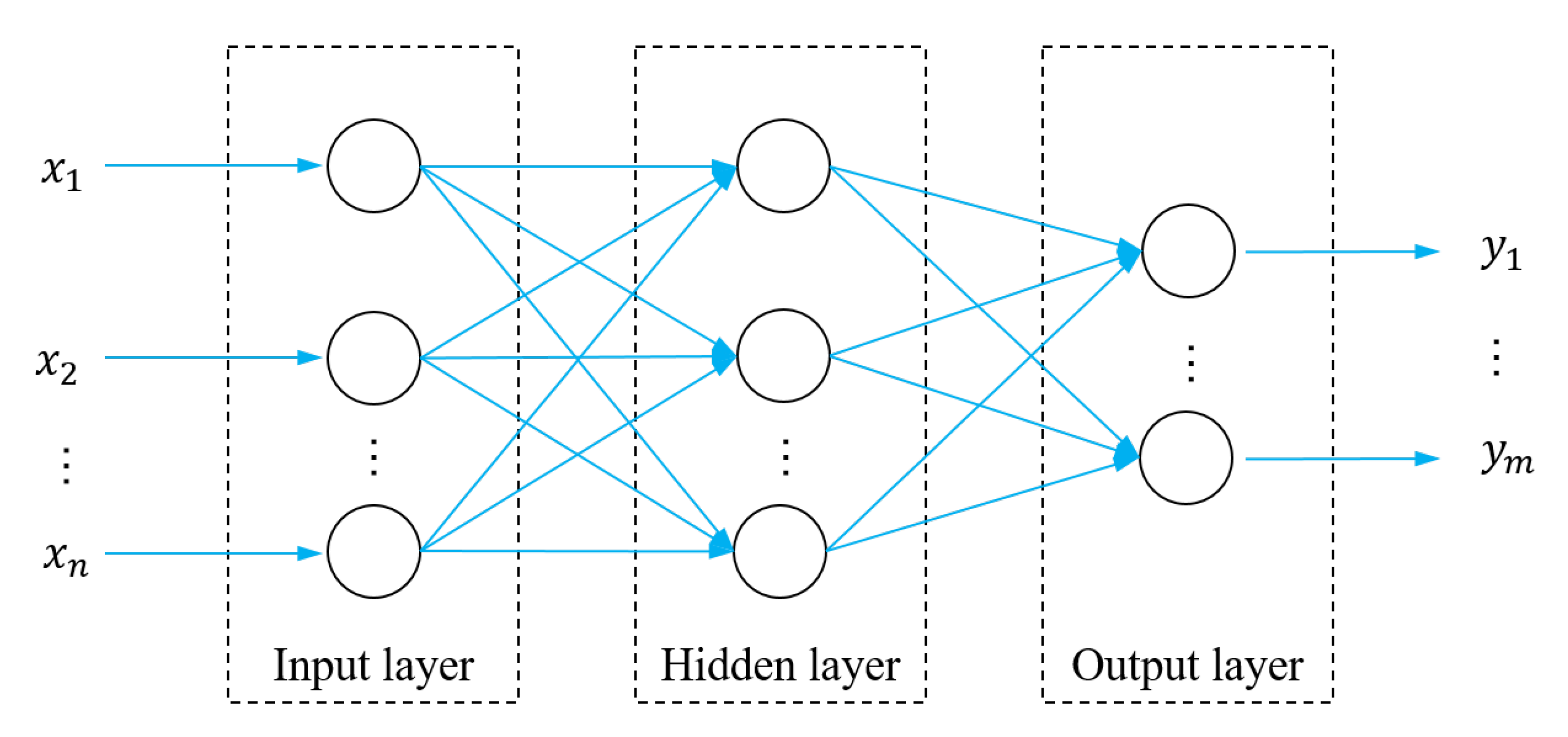
2.3.2. Radial Basis Functions Neural Network

RBFNN is a feedforward network model which consists of input layer, hidden layer and output layer, and its basic structure is shown in Figure 2. From the input layer to the hidden layer is a fixed non-linear transformation that maps the input vector directly into a new space. The mapping from the hidden layer space to the output layer space is linear, and the output layer implements a linear weighted combination in the new linear space, where the weight is the network adjustable parameter. The RBFNN does not need any mathematical assumptions and has the characteristics of a black box. It has a fast learning speed, a strong ability to predict complex nonlinear functions and excellent generalization ability.

For n dimensional input variables $x_1,x_2,\cdots ,x_n\in R$, the RBFNN can be expressed as:

$$y\left(x\right)={\displaystyle \sum }_{p=1}^p{\lambda }_p{\phi }_p\left(x\right)={\displaystyle \sum }_{p=1}^p{\lambda }_p{\phi }_p\left(\parallel x-x_j\parallel \right)$$

(21)

where $p$ is the number of neurons in the hidden layer, ${\lambda }_p$ is the weight factor, ${\phi }_p\left(x\right)$ is the p-th basis function of the hidden layer, and $\parallel x-x_j\parallel$ is the euclidean distance between the test point and the sample point.

The Gaussian basis function is used as the radial basis function of the neural network, which is expressed as:

$${\phi }_p\left(x\right)=\exp \left(-\frac{\parallel x-x_j\parallel {}^2}{2{\sigma }_p^2}\right)$$

(22)

2.3.3. Elliptical Basis Functions Neural Network

Kavuri et al. [29] have constructed the EBFNN based on the study of pattern recognition. The EBFNN uses hyperellipse to divide the design variable space, and the hidden layer neurons use the ellipse function as the basis function. The EBFNN is the same as the structure of the RBFNN. The EBFNN takes the Mahalanobis distance between the point to be measured and the sample point as the independent variable. For n dimensional input variables $x_1,x_2,\cdots ,x_n\in R$, the basis function can be expressed as:

$${\mathrm{g}}_i=\mathrm{g}\left(\parallel x-x_j\parallel {}_m\right)$$

(23)

$$\parallel x-x_j\parallel {}_m={\left(x-x_j\right)}^T{\mathit{S}}^{-1}\left(x-x_j\right) j=1,2,\cdots n$$

(24)

where $\mathit{S}$ is the covariance matrix. The EBFNN prediction model is constructed by linear superposition, and the input and output layers can be expressed as:

$$f_j^{in}\left(x\right)=1-{\displaystyle \sum }_{i=1}^n\frac{{\left(x_i-c_{ji}\right)}^2}{b_{ji}^2}$$

(25)

$$f_j^{out}\left(x\right)=\frac{e^{\beta }+1}{e^{\beta }}·\frac{1}{1+\exp \left(-\beta f_j^{in}\left(x\right)\right)}$$

(26)

where ${\mathrm{c}}_{ji}$, $b_{ji}$, respectively, represent the center value and semi-axis length of the ellipse element 𝑗 on the 𝑖-th dimension. $\beta$ is the adjustment parameter for the slope of the sigmoid curve. The larger the value of $\beta$, the faster the output value of the elliptic basis function tends to zero.

2.3.4. Error Analysis

The complex correlation coefficient R² is used to evaluate the consistency between the estimated value of the prediction model and the real value. It can be expressed as:

$$R^2=1-\frac{{{\displaystyle \sum }}_{i=1}^n{\left(y_i-{\widehat{y}}_i\right)}^2}{{{\displaystyle \sum }}_{i=1}^n{\left(y_i-\overline{y}\right)}^2}$$

(27)

where n is the number of sample points, $y_i$ is the actual value of the response, ${\widehat{y}}_i$ is the model estimated value, $\overline{y}$ is the average value of the actual value. When R² is closer to 1, the model accuracy is higher. It is generally considered that when the R² is above 0.9, the accuracy of the prediction model can meet the engineering needs [30].

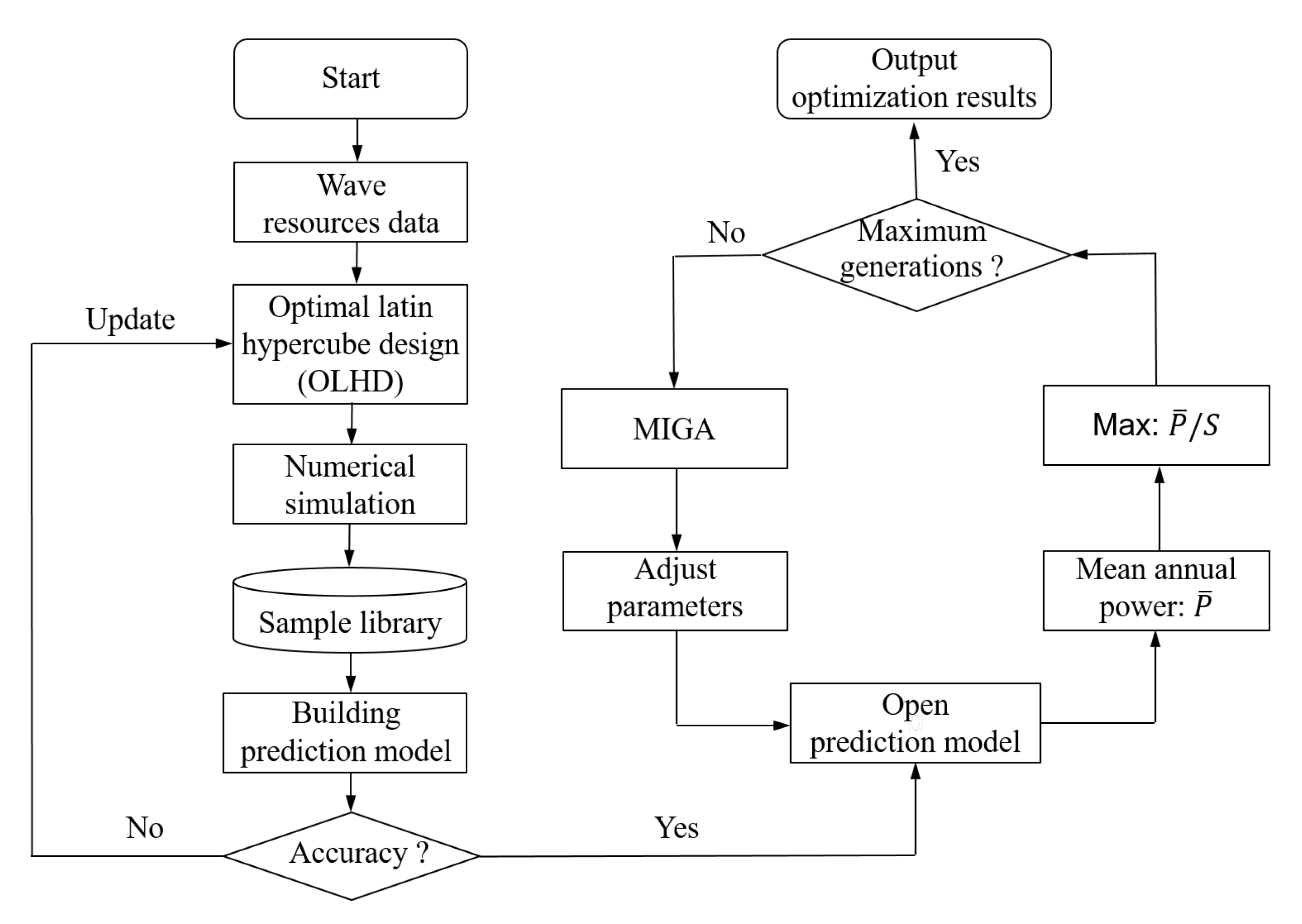
2.4. Optimization Algorithms and Processes

The origins of GA can be traced back to the early 1960s. The algorithm is designed and proposed according to the evolution law of organisms in nature. The GA imitates the genetic reproduction mechanism in the process of biological evolution, encodes the individuals in the solution space of the optimization problem, and then carries out genetic operations on the encoded individual population (such as selection, crossover, variation, etc.), and finds the combination containing the optimal solution or better solution from the new species population through iteration. GA is explained in detail in the works of Eiben and Smith [31].

The MIGA is an improvement of the parallel distributed genetic algorithm by Hiroyasu [32]. It divides a large population into several subpopulations, which are called “islands” vividly, and uses traditional GA algorithms to perform subpopulation evolution on each island. The schematic diagram is shown in Figure 3. The genetic evolution among the subpopulations does not interfere with each other. Every certain number of generations, some individuals are randomly selected to transfer to other islands, which helps complete the exchange of individuals between populations, and increase the diversity of individuals. Compared with GA, it can effectively suppress the occurrence of precocious phenomenon, which is beneficial to obtain the global optimal result [33].

The optimization process is illustrated in Figure 4. Some sample points are randomly selected in the design space by the optimal Latin hypercube design (OLHD). Calculating the hydrodynamic parameters (i.e., the wave excitation force, the additional mass, the radiation damping), the mean annual power for each sample point is calculated. The prediction model is established by analyzing the input and output variables of the sample library. When the prediction model meets the accuracy requirements, it is loaded into the optimization process. Then, the simulation calculation is replaced by the prediction model in the next optimization process. After initialization, according to the results of the previous generation, the parameters of the next-generation population individuals are obtained by genetic evolution. The individual parameters are input into the prediction model to obtain the energy capture power of the individual. The above process is repeated until the maximum generations and the population will contain the best individual after the maximum generations.

3. Building and Testing Prediction Models

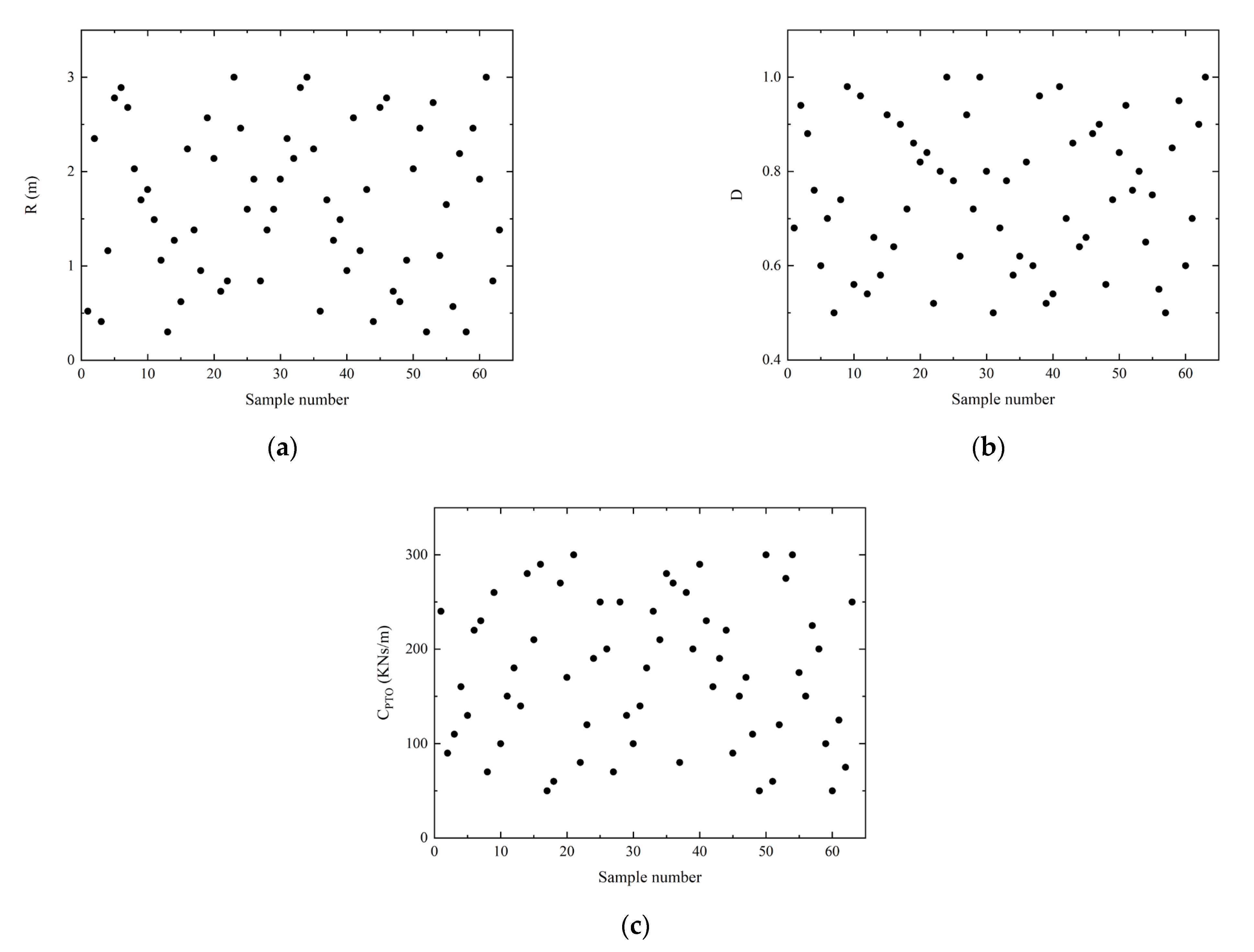
3.1. Sample Library

3.1.1. Determining the Design Space

In this paper, the WEC will be deployed in the sea near Chengshantou, Weihai, Shandong, China (123° E, 37.5° N). The wave resource statistics data were obtained from 2011 to 2020 by ERA5 reanalysis data [34]. The probability of occurrences of significant wave height and average wave period is shown in

Table 1. The average probability of occurrences of significant wave height and average wave period from 2011 to 2020.

Hs (m)	Tav (s)										Total
	2.5	3.5	4.5	5.5	6.5	7.5	8.5	9.5	10.5	11.5
0.25	3.25	14.00	7.37	2.64	0.77	0.16	0.07	0.03	0.01	0.00	28.30%
0.75	0.10	15.56	18.28	5.19	1.63	0.67	0.32	0.19	0.04	0.02	42.00%
1.25	0.00	0.54	10.88	3.37	0.46	0.14	0.08	0.02	0.02	0.02	15.53%
1.75	0.00	0.00	1.64	5.24	0.31	0.07	0.00	0.00	0.00	0.01	7.27%
2.25	0.00	0.00	0.02	2.76	0.89	0.03	0.00	0.00	0.00	0.00	3.70%
2.75	0.00	0.00	0.00	0.39	1.62	0.03	0.00	0.00	0.00	0.00	2.04%
3.25	0.00	0.00	0.00	0.01	0.79	0.08	0.00	0.00	0.00	0.00	0.88%
3.75	0.00	0.00	0.00	0.00	0.11	0.11	0.01	0.00	0.00	0.00	0.23%
4.25	0.00	0.00	0.00	0.00	0.00	0.05	0.00	0.00	0.00	0.00	0.05%
4.75	0.00	0.00	0.00	0.00	0.00	0.00	0.00	0.00	0.00	0.00	0.00%
Total	3.35%	30.10%	38.19%	19.60%	6.58%	1.34%	0.48%	0.24%	0.07%	0.05%	100%

. According to the statistics data, the average wave period concentrates in 3–6 s. the significant wave height mostly is less than 2 m.

The WEC captures wave energy through the movement of the buoy with the wave. Energy capture efficiency mainly depends on the shape of the buoy and the response of the PTO system [35,36]. Therefore, the radius R and the ratio of draft radius D and the damping coefficient C_PTO are selected as the optimization parameters.

(1)

The diameter of buoy is preferably 5–10% of the main wavelength [37]. Therefore, the value range of the buoy diameter can be expressed as follows:

$$0.6 \mathrm{m}<2R<6 \mathrm{m}$$

(28)

(2)

In order to ensure the rationality of the buoy shape, the draft of the buoy is normalized, which is expressed as D = H/R. The value range of D can be expressed as follows:

$$0.5<D<1$$

(29)

(3)

The traditional design method for the PTO system damping is based on the spectral peak frequency resonance, which leads to low energy capturing efficiency [20]. Therefore, the global search method is used to find the optimal PTO system damping which matches the wave resources. The value range of C_PTO can be expressed as follows:

$$50 \mathrm{KNs}/\mathrm{m}<C_{PTO}<300 \mathrm{KNs}/\mathrm{m}$$

(30)

According to the wave resources in the target sea area and considering the cost, the goal of this paper is to maximize the mean annual power per unit submerged surface area of the buoy [38]. Constraints and objective functions are as follows:

$$\begin{array}{cc}\max & \overline{P}/S\\ \begin{array}{c}s.t.\\ \\ \end{array}& \begin{array}{c}0.6 \mathrm{m}\le 2R\le 6 \mathrm{m}\\ 0.5\le D\le 1\\ 50 \mathrm{KNs}/\mathrm{m}\le C_{PTO}\le 300 \mathrm{KNs}/\mathrm{m}\end{array}\end{array}$$

(31)

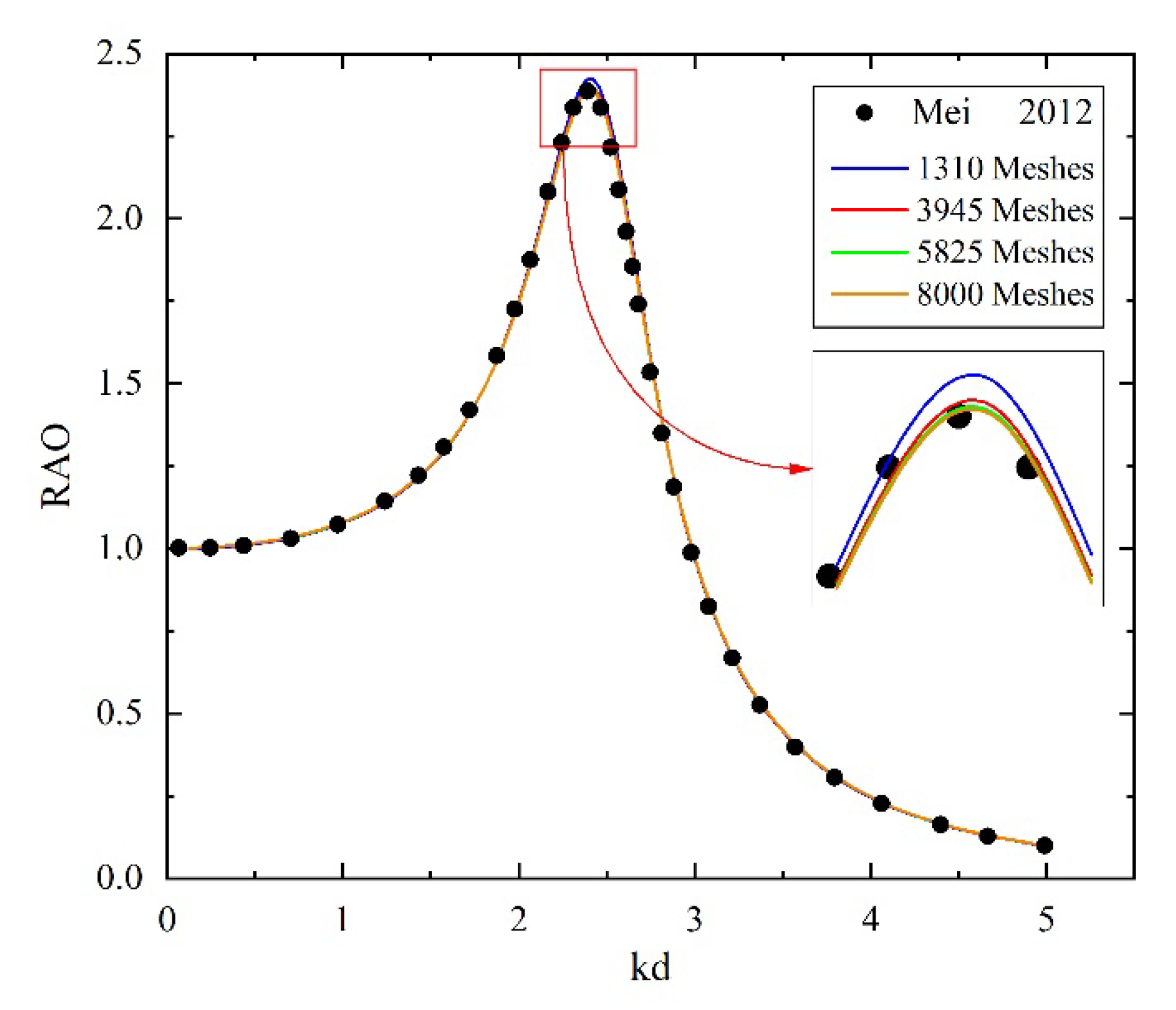
3.1.2. Hydrodynamic Calculation Verification

In order to verify the accuracy of simulation calculations and avoid the influence of the number of meshes on the simulation results, the numerical calculation results are compared with the results published in this paper by Mei [39]. The radius of the cylinder buoy is 4.05 m, the draft is 4.05 m. The wave frequency varies from 0.1 to 1.9 rad/s with an interval of 0.1 rad/s. k is the corresponding wave number. The water depth d is 15 m. The calculation meshes are 1310, 3945, 5825 and 8000, respectively. The calculated results are shown in Figure 5. When the total number of meshes are 1310, the response amplitude operator (RAO) peak calculation error is larger and the root mean square error (RMSE) is 0.021. When the number of meshes are 3945, 5825 and 8000, the RMSE is 0.017, 0.016 and 0.016, respectively. The calculation results tend to be consistent, and continuous refinement of the mesh has little effect on the simulation results. Therefore, in order to ensure high numerical simulation accuracy, the same mesh density is used.

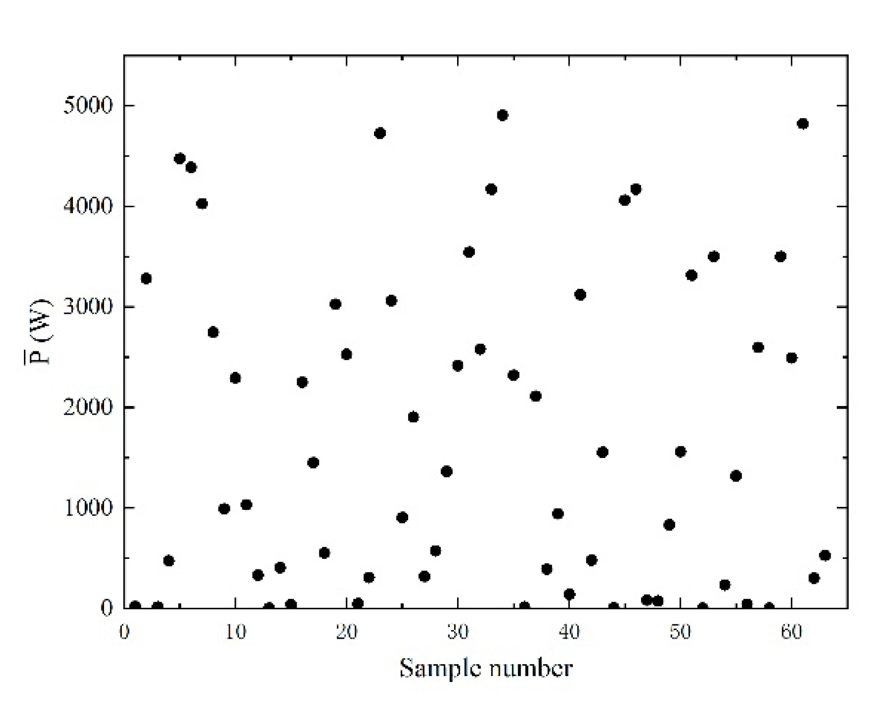
3.1.3. Calculating the Sample Points

The OLHD makes all test points as evenly distributed in the design space as possible, and has very good space filling and balance. The sample library is randomly selected in the design space by using OLHD, which covers 63 sample points [40]. The sample points are shown in

Table 2. Sample library.

Run#	R	D	CPTO	Run#	R	D	CPTO
1	0.52	0.68	240	33	2.89	0.78	240
2	2.35	0.94	90	34	3	0.58	210
3	0.41	0.88	110	35	2.24	0.62	280
4	1.16	0.76	160	36	0.52	0.82	270
5	2.78	0.6	130	37	1.7	0.6	80
6	2.89	0.7	220	38	1.27	0.96	260
7	2.68	0.5	230	39	1.49	0.52	200
8	2.03	0.74	70	40	0.95	0.54	290
9	1.7	0.98	260	41	2.57	0.98	230
10	1.81	0.56	100	42	1.16	0.7	160
11	1.49	0.96	150	43	1.81	0.86	190
12	1.06	0.54	180	44	0.41	0.64	220
13	0.3	0.66	140	45	2.68	0.66	90
14	1.27	0.58	280	46	2.78	0.88	150
15	0.62	0.92	210	47	0.73	0.9	170
16	2.24	0.64	290	48	0.62	0.56	110
17	1.38	0.9	50	49	1.06	0.74	50
18	0.95	0.72	60	50	2.03	0.84	300
19	2.57	0.86	270	51	2.46	0.94	60
20	2.14	0.82	170	52	0.3	0.76	120
21	0.73	0.84	300	53	2.73	0.8	275
22	0.84	0.52	80	54	1.11	0.65	300
23	3	0.8	120	55	1.65	0.75	175
24	2.46	1	190	56	0.57	0.55	150
25	1.6	0.78	250	57	2.19	0.5	225
26	1.92	0.62	200	58	0.3	0.85	200
27	0.84	0.92	70	59	2.46	0.95	100
28	1.38	0.72	250	60	1.92	0.6	50
29	1.6	1	130	61	3	0.7	125
30	1.92	0.8	100	62	0.84	0.9	75
31	2.35	0.5	140	63	1.38	1	250
32	2.14	0.68	180

, and the scatter diagrams of these samples are shown in Figure 6.

According to the sample points parameters, the simulation models are established. The wave excitation force, additional mass and radiation damping are calculated for each sample point based on ANSYS-AQWA. According to Equation (17), the mean annual power of each sample point was calculated, and the scatter diagrams are shown in Figure 7.

3.2. Training and Testing of the Prediction Model

The sample library is divided into two groups, respectively named as the training set and the validation set. The first 52 groups of sample points are used as the training set, and the last 11 groups of sample points are used as the verification set. The prediction models are trained based on RSM, RBFNN and EBFNN, respectively. When the buoy radius is constant, the mapping relationship between the PTO system damping, draft-to-radius ratio and mean annual power is shown in Figure 8.

The verification set is used to test the prediction performance of the three prediction models. The predicted value is compared with the numerical simulation calculation, and the results are shown in Figure 9. It can be seen intuitively from Figure 9 that the predicted values of the three prediction models are in good agreement with the actual values, and each point is distributed around the line $y=x$. Among the three prediction models, the EBF prediction model has the smallest error, and the RSM prediction model has the largest error. In addition to the use of test set verification, other evaluation methods are used. By Equation (27), the complex correlation coefficient R² of the training set is calculated. The R² of RSM prediction model is 0.99269. The R² of BFNN prediction model is 0.99913. The R² of EBFNN prediction model is 0.99963. The test results show that the obtained model could be used to predict the mean annual power.

4. Optimization Results and Discussion

Based on three prediction models, the MIGA is used to optimize the shape of the buoy. The population size is 60, the subpopulation size is 20, the number of subpopulations are 3, the number of generations are 100, the rate of crossover is 0.85, the rate of mutation is 0.01, the rate of migration is 0.01, and the interval generation of migration is 5. The optimization results are shown in Figure 10.

During the optimization process, the mean annual power is calculated by the prediction model. According to the calculation results of the previous generation, the optimization variables are continuously updated to form new generations, and the iterations are repeated until the maximum number of generations is reached. After 100 generations of evolution, the optimization results are shown in

Table 3. Optimization results.

Prediction Model	R (m)	D (m/m)	CPTO (KNs/m)	$\overline{\mathrm{P}}$/S (W/m2)	Simulation Result	Error
RSM	0.91	0.5	50	120.18	109.80	9.45%
RBFNN	1.56	0.5	50	119.10	126.08	5.54%
EBFNN	1.34	0.5	50	131.46	131.63	0.13%

.

As can be seen from Table 3, the comparison between optimization results and simulation results shows that the RSM prediction model has the lowest accuracy between the predicted value and the actual value, with an error of 9.45%. The RBFNN prediction model has the better accuracy by comparing the predicted value with the actual value, with an error of 5.54%. The EBFNN prediction model has the highest accuracy by comparing the predicted value with the actual value, with an error of 0.13%. The accuracy comparison of the three prediction models is the same as that of the corresponding complex correlation coefficient R². The accuracy of the prediction model established by the EBFNN method is the best, while the accuracy of the prediction model established by the RSM method is the worst.

In order to further verify the accuracy of the optimization results, the three design parameters are qualitatively analyzed respectively. The influence of these three parameters on $\overline{\mathrm{P}}$/S is analyzed by some simulation calculations. Figure 11 illustrates the response of $\overline{\mathrm{P}}$/S with buoy-shape parameters under optimal C_PTO. In Figure 11a, when the D is same, the $\overline{\mathrm{P}}$/S first increases and then decreases with the increase of the buoy radius. The $\overline{\mathrm{P}}$/S reaches peak when the radius is around 1.33 m. In Figure 11b, when the R is the same, the $\overline{\mathrm{P}}$/S decreases with the increase of the D. According to the change trend in Figure 11, it can be judged that the optimal parameters of the buoy are about when the R is 1.33 m and the draft is 0.665 m.

When the buoy is determined, the effect of C_PTO on the capture power of WEC is analyzed, as shown in Figure 12. In Figure 12a, when D is the same, the optimal C_PTO increases with the increase of R, and the smaller D, the faster the optimal C_PTO increases with the radius. In Figure 12b, when the R is the same, the optimal C_PTO decreases with the increase of the D, and the larger the radius, the faster the optimal C_PTO decreases with the increase of D. Since the wave energy is mainly distributed on the sea surface, wave force decays rapidly with increasing water depth. In Figure 12c, the $\overline{\mathrm{P}}$/S first increases and then decreases with the increase of C_PTO. In the design space, each set of shape parameters has an optimal C_PTO. According to the change trend in Figure 12, it can be judged that the optimal C_PTO is 50 KNs/m.

According to the comparison between the quantitative analysis results and the optimization results, it is found that the error of the optimization results of the RSM prediction model and the RBFNN prediction model is relatively large, and the error of the optimization results of the EBFNN prediction model is small, which further proves the reliability of the optimization results of the EBFNN prediction model.

The comparison of optimization results, numerical simulation results and qualitative analysis results shows that the EBFNN prediction model can reflect the function characteristics of input parameters and mean annual power most effectively. Combining the EBFNN prediction model with the MIGA to perform global optimization in the design space, it is easy to obtain high-performance buoy design parameters. When the prediction model method is adopted, only the sample points need to be calculated. After the prediction model meets the accuracy, the prediction model is used to replace the simulation calculation in the optimization process, and a total of 63 simulation calculations are required. When the direct optimization design method is adopted, it is necessary to perform simulation calculations on the newly generated population individuals, and then the genetic variation generates the next-generation population. This iteration is repeated until the optimization generations are reached, which requires a total of 6300 simulation calculations. Obviously, the number of repeated modeling and simulation calculations required by the prediction model method is only 1% of the direct optimization design, and correspondingly, 99% of the original workload can be saved. The comparison between the prediction model optimization design method and the direct optimization design shows that the prediction model replacing the simulation calculation method can effectively reduce the number of repeated simulation calculations in the optimization process, effectively shortening the optimization design cycle, and improving the optimization design efficiency.

5. Conclusions

In order to further improve the capture efficiency of WEC, this paper focuses on the optimization design of the buoy shape. In view of the shortcomings of traditional optimization methods such as long-time consumption and low optimization efficiency, this paper discusses the feasibility of using prediction models to replace simulation calculations. The method uses a small number of experimental samples to build a prediction model. In the optimization process, it replaces the actual model, which greatly reduces the evaluation and computation of the objective function and constraint function. Aiming at the shortcomings of RSM and RBFNN to establish the prediction model, the EBFNN is proposed to train the prediction model. The prediction models obtained by the three methods are combined with MIGA to conduct global optimization in the design space. The obtained optimization results are compared with the simulation calculation results and qualitative analysis results, and the following conclusions can be obtained:

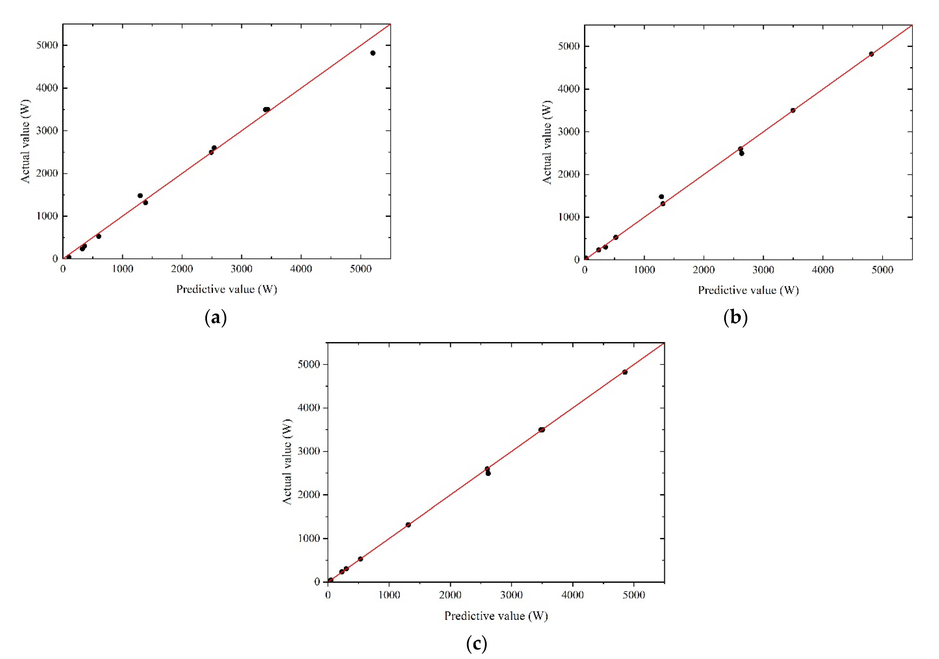
(1)

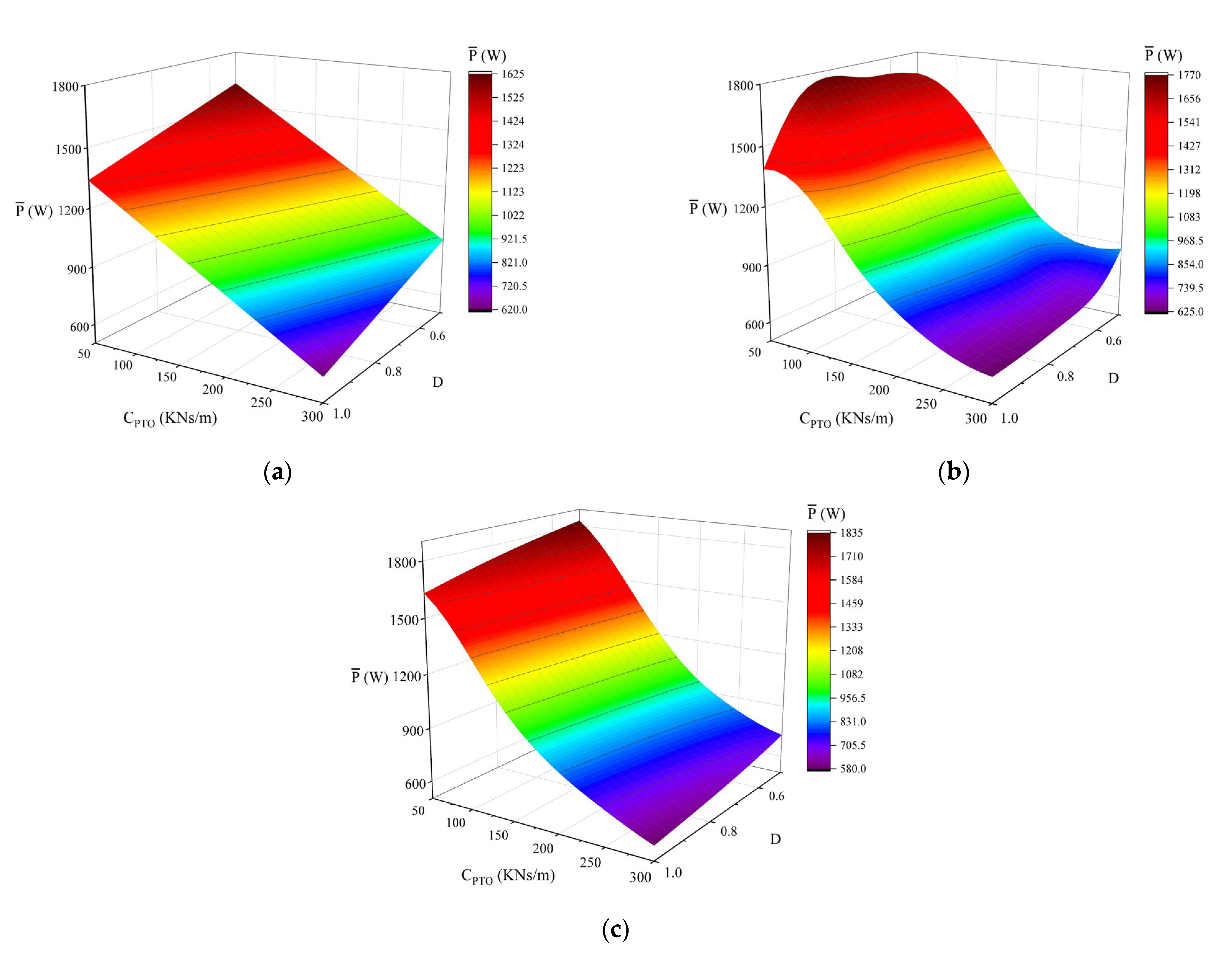
The comparison shows that the prediction model established by the RSM method has the worst accuracy, the prediction model trained by the RBFNN method has better accuracy, and the prediction model trained by the EBFNN method has the best accuracy. The mean annual power prediction model trained by the EBFNN method can more accurately reflect the mapping relationship between the input and output. According to the shape parameters of the buoy, the mean annual power can be accurately predicted.

(2)

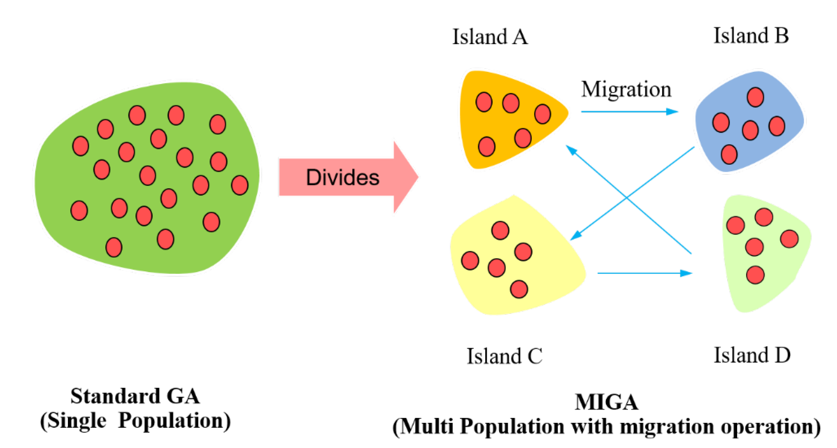
Taking the wave statistics data of the Chengshantou sea area near Weihai City, Shandong Province, China, as an example, the method of combining MIGA and the mean annual prediction model is adopted to obtain a high-performance design scheme, which provides a reference for engineering design. In the optimization process, the mean annual power prediction model replaces the simulation calculation, which can reduce a lot of workload (i.e., repeated modeling, simulation, and calculation). Compared with optimization design based on simulation results, this method can save considerable time and cost, effectively shorten the optimization design cycle, and improve the optimization efficiency. This optimization method can also be extended to the optimal design of other sea areas or types of WECs. In the future, we will continue to explore WEC array optimization methods. In order to promote the development of WEC commercialization, WEC array optimization methods will be investigated in the future.

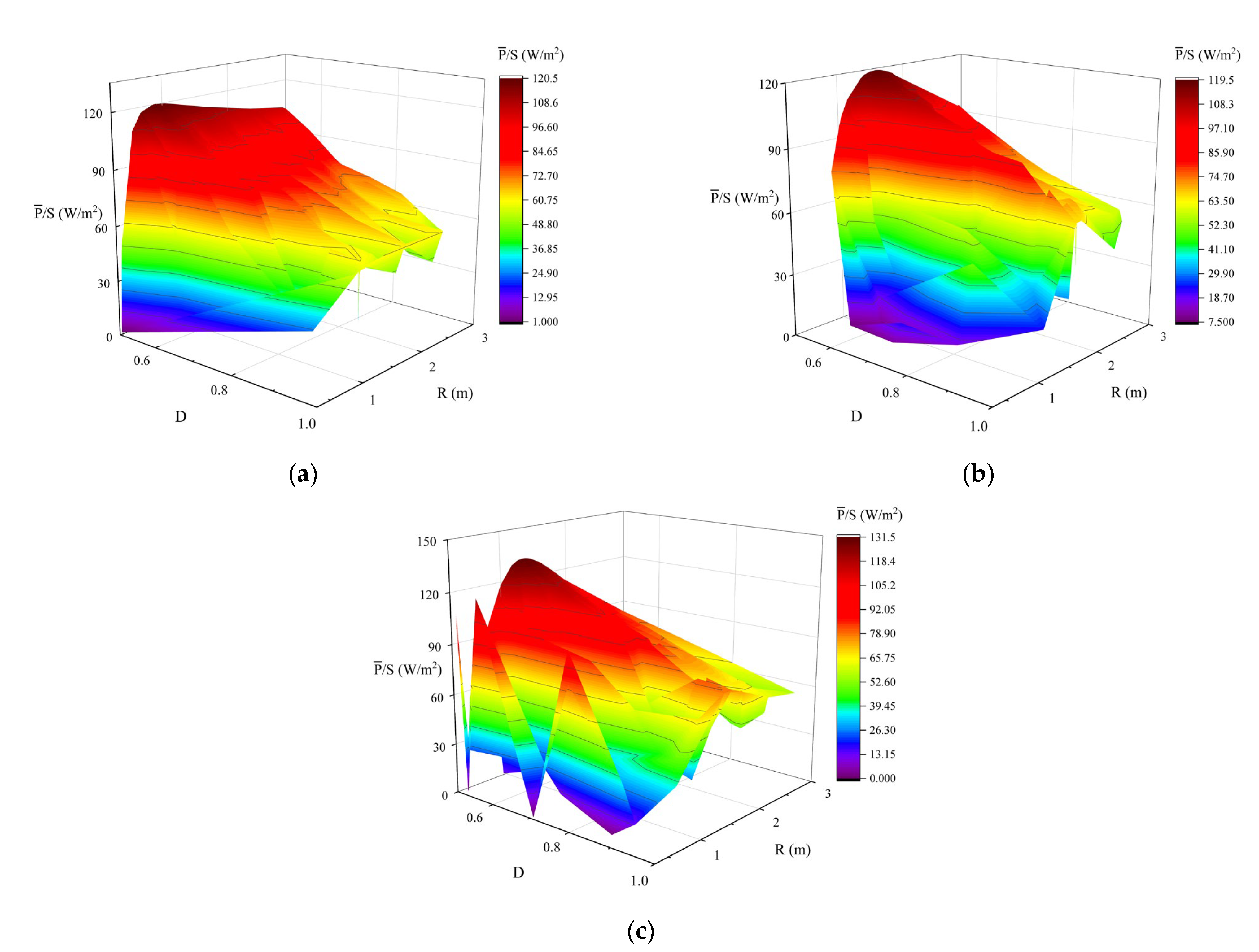
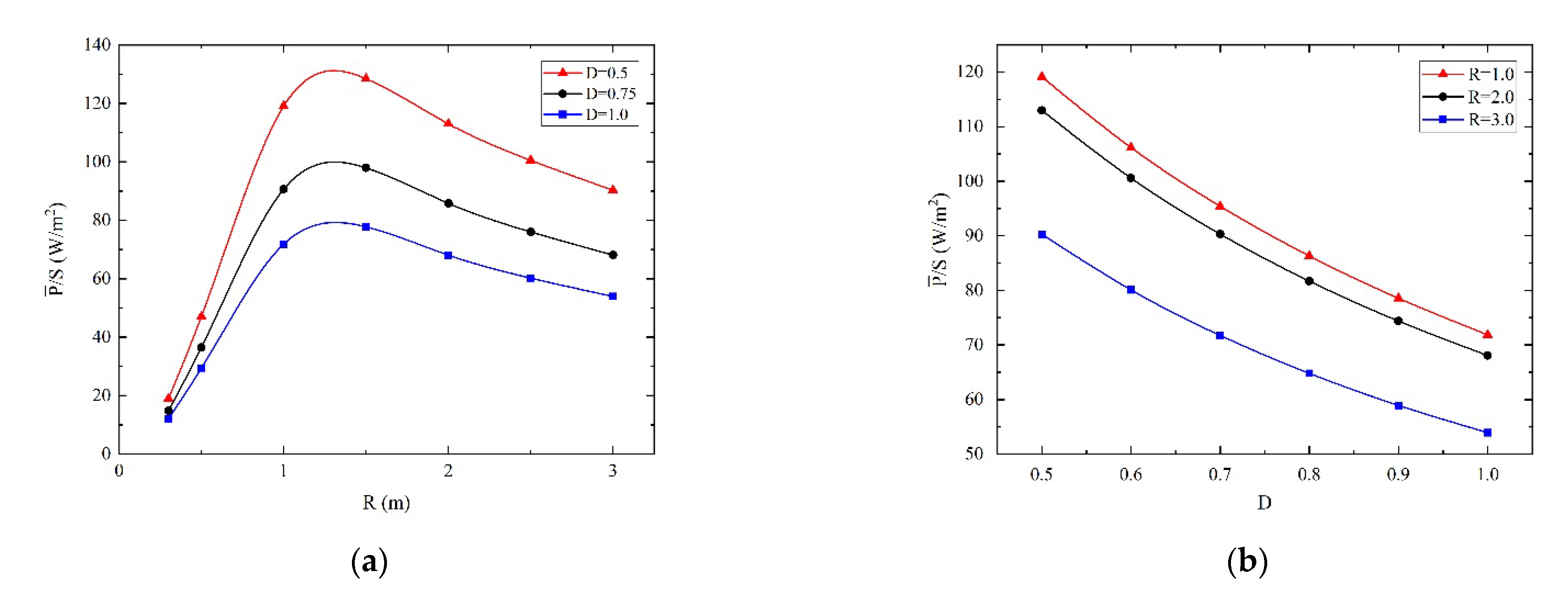
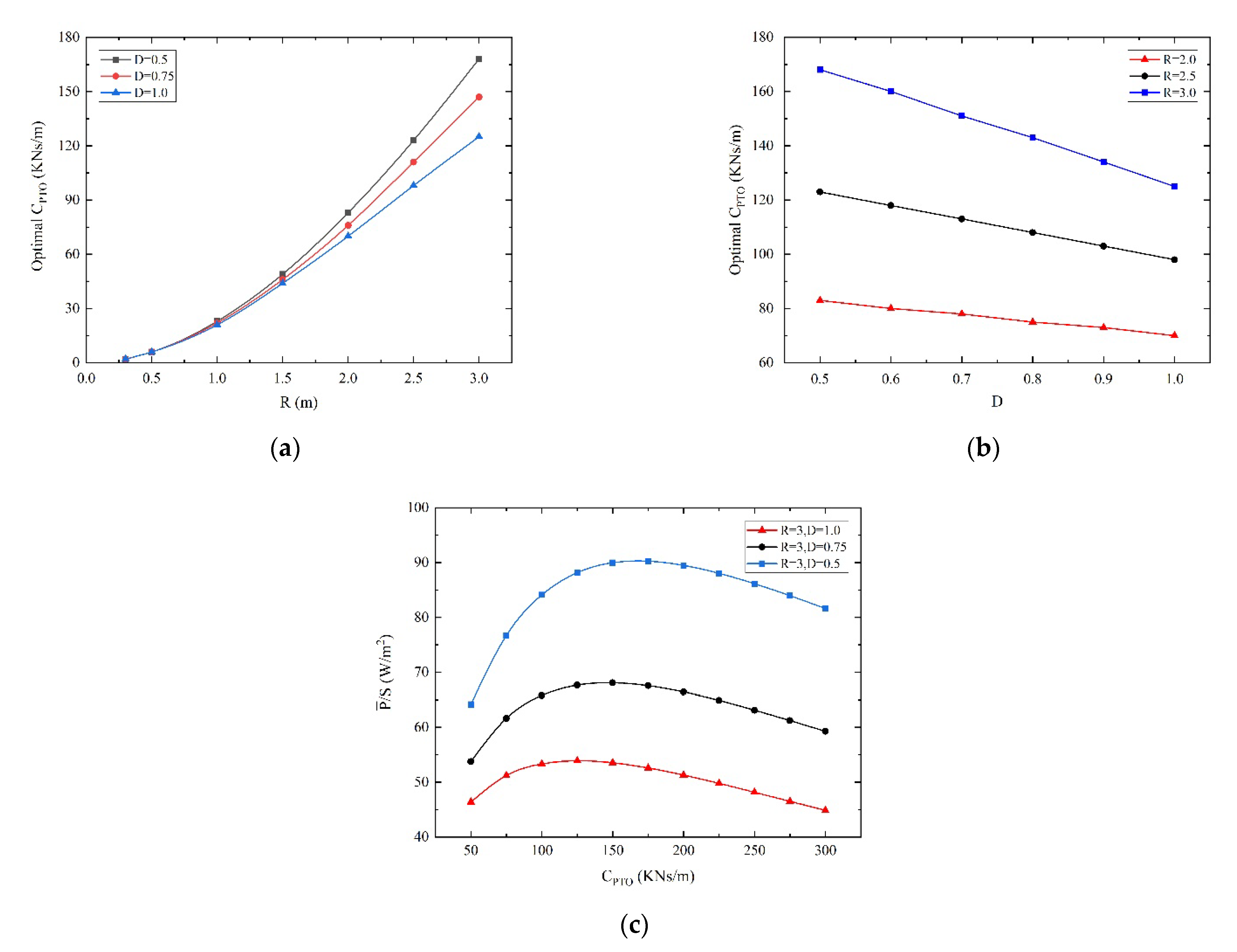
(3)

The three optimization parameters have a significant impact on the energy capture performance. When the buoy shape is determined, the $\overline{\mathrm{P}}$/S first increases and then decreases with the increase of damping, and there is an optimal C_PTO. The optimal C_PTO is significantly affected by buoy radius and draft, which is positively correlated with the buoy radius and negatively correlated with the buoy draft. When C_PTO is the optimal damping, the $\overline{\mathrm{P}}$/S increases first and then decreases with the increase of radius and the $\overline{\mathrm{P}}$/S decreases with the increase of draft.

References

- Mathiesen, B.V.; Lund, H.; Karlsson, K. 100% Renewable energy systems, climate mitigation and economic growth. Appl. Energy 2011, 88, 488–501. [Google Scholar] [CrossRef]
- Panwar, N.L.; Kaushik, S.C.; Kothari, S. Role of renewable energy sources in environmental protection: A review. Renew. Sustain. Energy Rev. 2011, 15, 1513–1524. [Google Scholar] [CrossRef]
- Pecher, A.; Kofoed, J.P. Handbook of Ocean Wave Energy, 1st ed.; Springer Nature: Cham, Switzerland, 2017; pp. 19–34. [Google Scholar]
- Nguyen, H.P.; Wang, C.M.; Tay, Z.Y.; Luong, V.H. Wave Energy Converter and Large Floating Platform Integration: A Review. Ocean Eng. 2020, 213, 107768. [Google Scholar] [CrossRef]
- Zhao, C.Y.; Cao, F.F.; Shi, H.D. Optimisation of heaving buoy wave energy converter using a combined numerical model. Appl. Ocean Res. 2020, 102, 102208. [Google Scholar] [CrossRef]
- Hantoro, R.; Septyaningrum, E.; Hudaya, Y.R.; Utama, I. Stability analysis for trimaran pontoon array in wave energy converter–pendulum system (WEC-PS). Brodogradnja 2022, 73, 59–68. [Google Scholar] [CrossRef]
- Legaz, M.J.; Soares, C.G. Evaluation of various wave energy converters in the bay of Cádiz. Brodogradnja 2022, 73, 57–88. [Google Scholar] [CrossRef]
- Jin, S.; Greaves, D. Wave energy in the UK: Status review and future perspectives. Renew. Sustain. Energy Rev. 2021, 143, 110932. [Google Scholar] [CrossRef]
- Farkas, A.; Degiuli, N.; Martić, I. Assessment of Offshore Wave Energy Potential in the Croatian Part of the Adriatic Sea and Comparison with Wind Energy Potential. Energies 2019, 12, 2357. [Google Scholar] [CrossRef] [Green Version]
- Weber, J.; Mouwen, F.; Parish, A.; Robertson, D. Wavebob-Research & Development Network and Tools in the Context of Systems Engineering. In Proceedings of the 8th European Wave Tidal Energy Conference, London, UK, 15–16 November 2009; pp. 416–420. [Google Scholar]
- Falcão, A.F.O. Wave energy utilization: A review of the technologies. Renew. Sustain. Energy Rev. 2010, 14, 899–918. [Google Scholar] [CrossRef]
- Goggins, J.; Finnegan, W. Shape optimisation of floating wave energy converters for a specified wave energy spectrum. Renew. Energy 2014, 71, 208–220. [Google Scholar] [CrossRef]
- Shi, H.D.; Han, Z.H.; Zhao, C.Y. Numerical study on the optimization design of the conical bottom heaving buoy convertor. Ocean Eng. 2019, 173, 235–243. [Google Scholar] [CrossRef]
- Berenjkoob, M.N.; Ghiasi, M.; Soares, C.G. Influence of the shape of a buoy on the efficiency of its dual-motion wave energy conversion. Energy 2021, 214, 118998. [Google Scholar] [CrossRef]
- Shadman, M.; Estefen, S.F.; Rodriguez, C.A.; Nogueira, I.C.M. A geometrical optimization method applied to a heaving point absorber wave energy converter. Renew. Energy 2018, 115, 533–546. [Google Scholar] [CrossRef]
- Wu, J.M. Geometry Optimization of Heaving Axisymmetric Point Absorbers under Parametrical Constraints in Irregular Waves. J. Mar. Sci. Eng. 2021, 9, 1136. [Google Scholar] [CrossRef]
- McCabe, A.P.; Aggidis, G.A.; Widden, M.B. Optimizing the shape of a surge-and-pitch wave energy collector using a genetic algorithm. Renew. Energy 2010, 35, 2767–2775. [Google Scholar] [CrossRef]
- Garcia-Teruel, A.; DuPont, B.; Forehand, D.I.M. Hull geometry optimisation of wave energy converters: On the choice of the objective functions and the optimisation formulation. Appl. Energy 2021, 298, 117153. [Google Scholar] [CrossRef]
- Neshat, M.; Sergiienko, N.; Mirjalili, S.; Nezhad, M.M.; Piras, G.; Garcia, D.A. Multi-Mode Wave Energy Converter Design Optimisation Using an Improved Moth Flame Optimisation Algorithm. Energies 2021, 14, 3737. [Google Scholar] [CrossRef]
- Ji, T.; Cao, F.F.; Dong, X.C.; Li, D.M.; Shi, H.D. Optimized design of 3-DOF buoy wave energy converters under a specified wave energy spectrum. Appl. Ocean Res. 2021, 116, 102885. [Google Scholar] [CrossRef]
- Koh, H.J.; Ruy, W.S.; Cho, I.H.; Kweon, H.M. Multi-objective optimum design of a buoy for the resonant-type wave energy converter. J. Mar. Sci. Technol. 2015, 20, 53–63. [Google Scholar] [CrossRef]
- Colby, M.K.; Nasroullahi, E.M.; Tumer, K. Optimizing Ballast Design of Wave Energy Converters Using Evolutionary Algorithms. In Proceedings of the 13th Annual Conference on Genetic and Evolutionary Computation, Dublin, Ireland, 12–16 July 2011; pp. 1739–1746. [Google Scholar]
- Avila, D.; Marichal, G.N.; Quiza, R.; Luis, F.S. Prediction of Wave Energy Transformation Capability in Isolated Islands by Using the Monte Carlo Method. J. Marine Sci. Eng. 2021, 9, 980. [Google Scholar] [CrossRef]
- Avila, D.; Marichal, G.N.; Padrón, I.; Quiza, R.; Hernández, A. Forecasting of wave energy in Canary Islands based on artificial intelligence. Appl. Ocean Res. 2020, 101, 102–189. [Google Scholar] [CrossRef]
- Wang, W.; Liu, Y.J.; Bai, F.G.; Xue, G. Capture Power Prediction of the Frustum of a Cone Shaped Floating Body Based on BP Neural Network. J. Marine Sci. Eng. 2021, 9, 656. [Google Scholar] [CrossRef]
- Liu, Z.; Wang, Y.; Hua, X. Prediction and optimization of oscillating wave surge converter using machine learning techniques. Energy Convers. Manag. 2020, 210, 112677. [Google Scholar] [CrossRef]
- Perez, T. Ship Motion Control: Course Keeping and Roll Stabilisation Using Rudder and Fins; Springer: Berlin/Heidelberg, Germany, 2006. [Google Scholar]
- McCabe, A. Constrained optimization of the shape of a wave energy collector by genetic algorithm. Renew. Energy 2013, 51, 274–284. [Google Scholar] [CrossRef]
- Kavuri, S.N.; Venkatasubramanian, V. Using fuzzy clustering with ellipsoidal units in neural networks for robust fault classification. Comput. Chem. Eng. 1993, 17, 765–784. [Google Scholar] [CrossRef]
- Wang, J.; Pang, Y.J.; Cheng, Y.X.; Yang, Z.Y.; Liu, W. Application of prediction models to optimize the design of the non-uniform ring-frames pressure shell. J. Ship Mech. 2014, 18, 1331–1338. [Google Scholar] [CrossRef]
- Eiben, A.E.; Smith, J.E. Introduction to Evolutionary Computing, 1st ed.; Springer: Berlin/Heidelberg, Germany, 2003; pp. 37–69. [Google Scholar]
- Miki, M.; Hiroyasu, T.; Kaneko, M.; Hatanaka, K. A Parallel Genetic Algorithm with Distributed Environment Scheme. In Proceedings of the 1999 IEEE International Conference on Systems, Man, and Cybernetics, Tokyo, Japan, 12–15 October 1999; pp. 695–700. [Google Scholar]
- Zhang, W.W.; Qi, H.; Yu, Z.Q.; He, M.J.; Ren, Y.T.; Li, Y. Optimization configuration of selective solar absorber using multi-island genetic algorithm. Sol. Energy 2021, 224, 947–955. [Google Scholar] [CrossRef]
- ECMWF. Available online: https://www.ecmwf.int/en/forecasts/datasets/reanalysis-datasets/era5 (accessed on 13 December 2021).
- Bhatta, D.D.; Rahman, M. On scattering and radiation problem for a cylinder in water of finite depth. Int. J. Eng. Sci. 2003, 41, 931–967. [Google Scholar] [CrossRef]
- Chen, Z.F.; Zhou, B.Z.; Zhang, L.; Sun, L.; Zhang, X.W. Performance evaluation of a dual resonance wave-energy convertor in irregular waves. Appl. Ocean Res. 2018, 77, 77–88. [Google Scholar] [CrossRef]
- Falnes, J.; Perlin, M. Ocean waves and oscillating systems: Linear interactions including wave-energy extraction. Appl. Mech. Rev. 2003, 56, B3. [Google Scholar] [CrossRef]
- Garcia-Teruel, A.; Forehand, D.I.M. A review of geometry optimisation of wave energy converters. Renew. Sustain. Energy Rev. 2021, 139, 110593. [Google Scholar] [CrossRef]
- Mei, C.C. Hydrodynamic principles of wave power extraction. Phil. Trans. R. Soc. A 2012, 370, 208–234. [Google Scholar] [CrossRef]
- Chen, W.; Jin, R.C.; Sudjianto, A. Analytical Global Sensitivity Analysis and Uncertainty Propagation for Robust Design. J. Qual. Technol. 2006, 38, 333–348. [Google Scholar] [CrossRef]