Elliptical-Shaped Fresnel Lens Design through Gaussian Source Distribution

Abstract

A novel three-dimensional elliptical-shaped Fresnel lens (ESFL) analytical model is presented to evaluate and maximize the solar energy concentration of Fresnel-lens-based solar concentrators. AutoCAD, Zemax and Ansys software were used for the ESFL design, performance evaluation and temperature calculation, respectively. Contrary to the previous modeling processes, based on the edge-ray principle with an acceptance half-angle of ±0.27° as the key defining parameter, the present model uses, instead, a Gaussian distribution to define the solar source in Zemax. The results were validated through the numerical analysis of published experimental data from a flat Fresnel lens. An in-depth study of the influence of several ESFL factors, such as focal length, arch height and aspect ratio, on its output performance is carried out. Moreover, the evaluation of the ESFL output performance as a function of the number/size of the grooves is also analyzed. Compared to the typical 1–16 grooves per millimeter reported in the previous literature, this mathematical parametric modeling allowed a substantial reduction in grooves/mm to 0.3–0.4, which may enable an easy mass production of ESFL. The concentrated solar distribution of the optimal ESFL configuration was then compared to that of the best flat Fresnel lens configuration, under the same focusing conditions. Due to the elliptical shape of the lens, the chromatic aberration effect was largely reduced, resulting in higher concentrated solar flux and temperature. Over 2360 K and 1360 K maximum temperatures were found for ESFL and flat Fresnel lenses, respectively, demonstrating the great potential of the three-dimensional curved-shaped Fresnel lens on renewable solar energy applications that require high concentrations of solar fluxes and temperatures.

1. Introduction

Optical concentration provides strong cost leverage for photovoltaic cells [1]. High concentrated photovoltaic technology uses relatively inexpensive optics, such as mirrors and lenses, to concentrate sunlight from a broad area into a much smaller area of active semiconductor cell and converts sunlight directly to electricity [2,3]. The Fresnel lens has been widely used in the concentrated photovoltaic field, with the advantages of simple structure, light weight, low cost, easy processing, etc. [4]. However, it has a limited concentration ratio due to its strong chromatic aberration.

To overcome this issue, non-flat Fresnel lenses have been widely studied by many researchers, proposing new modeling methods and configurations with the aim of increasing the solar energy concentration. The shaped Fresnel lens conception was initiated in 1977 by Cosby [5]. One year later, a patent was filed by O’Neill [6], while Kritchman published his finding [7]. Since then, many other researchers throughout the world have been proposing their own non-flat Fresnel lens models and modeling processes [8,9,10,11,12,13]. Currently, the most notable work in this field is a published book by Leutz et al. [14], who presented an in-depth study of the non-flat shaped Fresnel lens.

The modeling process of the shaped Fresnel lens follows Snell’s law (or law of refraction). The half-angle subtended by the Sun is the key parameter to set the size of the refractive prism facets by using the edge-ray principle, which adjusts the number of grooves required for the concentrator. It dictates the absolute angle at which the solar rays arrive at the surface of the Earth globe. The Sun–Earth subtended acceptance half-angle of 0.27° can be determined by the mathematical relationship between the radial size of the Sun and its distance to the Earth [15,16,17]. It stands valid from a theoretical and mathematical perspective, being considered by many researchers in the field of solar energy concentration [7,8,9,10,11,12,14,15,16,17,18,19,20,21,22,23]. However, this angle could only be accepted if the Earth had no atmosphere. The sudden change from vacuum to Earth’s atmosphere significantly alters the trajectory of solar rays due to the law of refraction. The solar rays pass through various atmospheric layers, such as the thermosphere, mesosphere, stratosphere, and troposphere. Each individual layer’s gaseous composition has its own refractive index, influencing the refraction angle. Moreover, the half-angle subtended by the Sun can be different depending on geographical location, time zone, and local atmospheric conditions, such as the presence of clouds, humidity, sand particles and pollution in the troposphere. Therefore, within the Earth’s atmosphere, the acceptance half-angle should be larger than 0.27°. These complex systems that influence the refraction of sunlight on Earth were neglected by most researchers in this field, who had adopted the half-angle of 0.27° as a standard for their works [7,8,9,10,11,12,14,15,16,17,18,19,20,21,22,23,24]. This oversimplification in the acceptance half-angle calculation paired with the edge-ray principle has set and cemented the number and size of grooves in the production of Fresnel lenses in the market [25].

There are two categories of simulation methods for evaluation of the concentration systems: one by ray tracing and the other by analytical approach [26,27]. The ray-tracing method simulates a vast number of discrete and well-defined rays of different wavelength, energy and traveling trajectory. Each ray has its own trajectory, which is influenced by the transmission, reflection, or refraction in a medium within its path. It is only numerically completed when the ray hits an absorbing detector or reaches an annihilation condition. This category has an accurate prediction of the flux distribution, but with the cost of high computing complexity, power and time. Several pre-existing reputable ray-tracing tools are available in the market, such as Zemax [28,29,30], LightTools [19,31,32,33] and Soltrace [34]. These software are reliable, robust, user friendly, easy to learn and allow repeatability, making them great tools to expand new fields of research.

The analytical method describes the flux density distribution through self-written complex computational codes and programs. This undoubtedly decreases significantly the computing time and has been widely adopted [8,9,10,12,21,22]. However, each research group has its own source code, which could be vastly different from that of another. In addition, there are no guarantees that the written code has been implemented correctly or that all the essential parameters and functions have been included. Due to all these uncertainties, the results could also be significantly different from each other.

The detailed description and analysis of the focusing image is the backbone of solar concentration research. The maximum attainable concentration and the flux distribution at the focal zone are some of the few characteristics that should be thoroughly explored and meticulously presented. To ensure the validity of the numerical or analytical results, it should be experimentally verified or compared to an existing experiment.

In this work, a parametric modeling procedure of a three-dimensional elliptical-shaped Fresnel lens (ESFL) is presented, using Snell’s law. The ESFL is designed in AutoCAD, and then imported into Zemax nonsequential ray-tracing software for numerical evaluation of the ESFL output performance. In this evaluation, a Gaussian distribution based on measured data from the literature [35] is considered to define the solar source, instead of the classical edge-ray principle method with a solar acceptance half-angle of 0.27°. To validate the analytical model, this was applied in the performance evaluation of a flat Fresnel lens with published experimental data [36], whose results were in accordance with those obtained through the proposed model. An in-depth study of the influence of the ESFL parameters, such as focal length, arch height and aspect ratio on its output performance, in terms of concentrated solar flux, optical efficiency and full width at half maximum (FWHM), is also carried out. Furthermore, to the best of our knowledge, this is the first time that the ESFL concentration efficacy is evaluated as a function of the number of grooves, with optimal 0.4–0.3 groove numbers per millimeter being found. This study reveals that the number of grooves necessary to maximize the concentrated solar flux could be significantly reduced in relation to that reported by the literature and market, which may enhance the cost efficiency of the manufacturing process of Fresnel lens solar concentrators. From the abovementioned studies, the best ESFL design is found. The optimal concentrated solar flux value within its focal cone is then analyzed and compared to that of a flat Fresnel lens, which proved the effectiveness of the ESFL in substantially reducing the chromatic aberration and, consequently, on maximizing the solar flux. The temperature analysis of both concentrators is also performed by Ansys. The maximum temperatures of 2360 K and 1360 K are attained from the ESFL and the flat Fresnel lens, respectively, demonstrating once more the potential of the ESFL in many solar energy research and applications that require high solar flux and temperature.

2. Modeling of an Elliptical-Shaped Fresnel Lens

The ESFL model has an elliptical-shaped arch with a smooth surface facing the Sun and grooves on the opposite side, as shown in Figure 1. This guarantees the easier cleaning of the lens in case of dirt, without damaging the grooves.

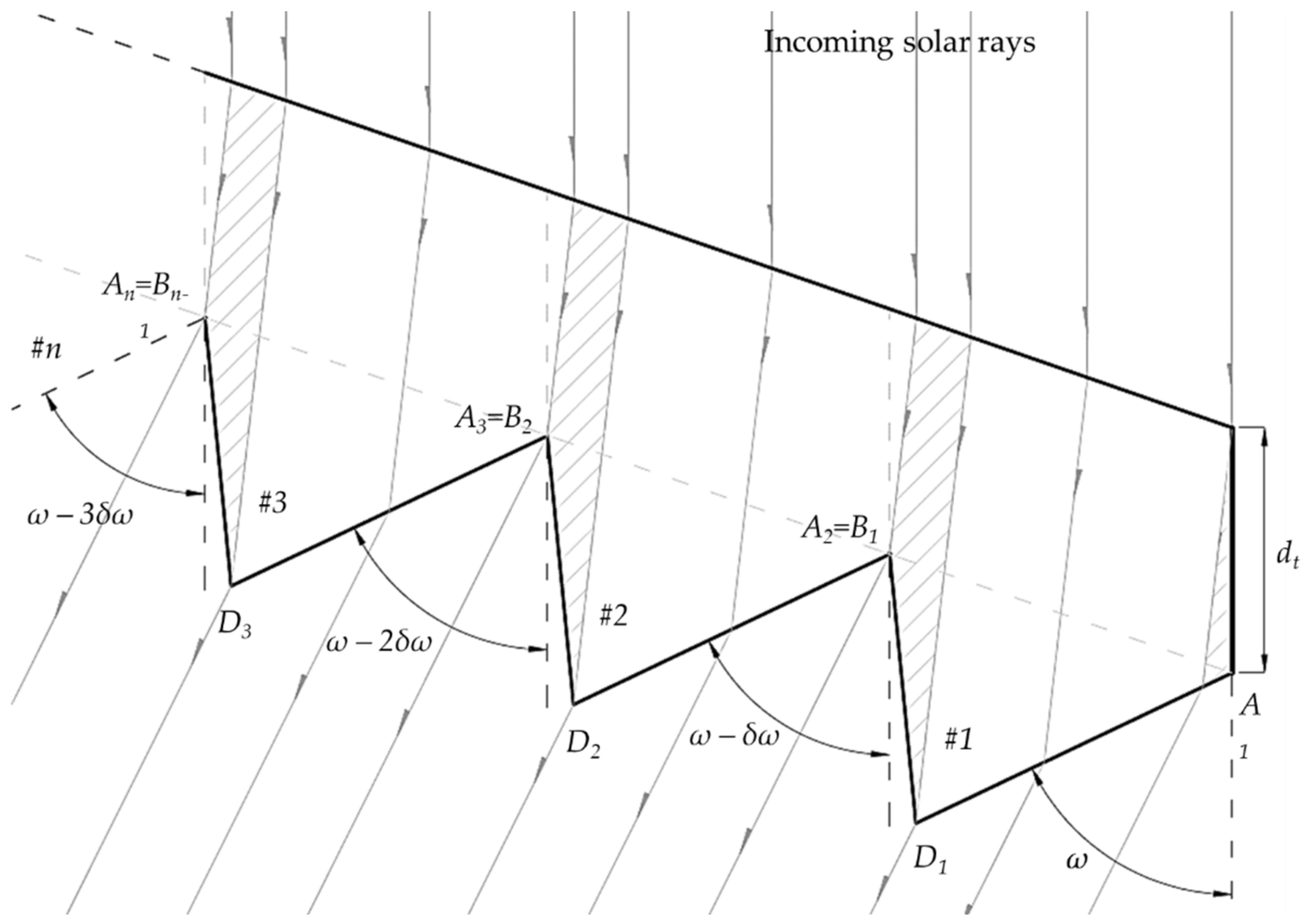
2.1. Analytical Method

The design of the ESFL followed a generic ellipse Equation (1), represented in Figure 2.

$$\frac{x^2}{a^2}+\frac{y^2}{b^2}=1,$$

(1)

As shown in Figure 2, the conception of the elliptical arch depends on the radius or aperture of the concentrator (r), its focal height (h_f) and the height of the arch (h_l). The angle ω is the aperture angle or rim angle of the concentrator, with h_f and r defining its size. The ellipse’s major axis “a” and minor axis “b” can be both calculated with those variables through Equation (2). The minor axis “b” is the combination of h_f and h_l and, once it is found, the major axis “a” can be acquired.

$$\left\{\begin{array}{c}a=\frac{b\times r}{\sqrt{b^2-h_f{}^2}}\\ b=h_f+h_l\end{array}\right.,$$

(2)

The ESFL can be considered as a set of well-defined and positioned prisms, as shown in Figure 3.

The prisms were modeled through Equation (3), based on Snell’s law, starting with the outmost one, as indicated in Figure 3a. Each prism is defined by three facets: the input, output and back facets, represented in Figure 3b. The input facet is defined by the segment between point A and point B. α represents the angle between the vertical line (solar ray path), with the normal line of the input facet AB. The solar ray is refracted as it hits AB. Depending on the refractive index of the medium (n_λ), the ray is deviated by an angle γ. It is then shifted further as its leaves the output facet of the prism, making an angle of ω in relation to the vertical axis. The output facet is either defined by the segment AC or AD depending on the pitch angle. In this paper, the refractive index n_λ of poly (methyl methacrylate) (PMMA) material (n_λ = 1.492) was considered.

$$\left\{\begin{array}{c}\sin \left(\alpha \right)=n_{\lambda }\sin \left(\alpha -\gamma \right)\\ n_{\lambda }\sin \left(\beta +\gamma \right)=\sin \left(\beta +\omega \right)\end{array}\right.,$$

(3)

The number of prisms/grooves (N) was calculated through Equation (4), where δω is the groove division angle, which represents a small angular segment of the elliptical Fresnel lens.

$$N=\frac{\omega }{\delta \omega },$$

(4)

Equations (5) and (6) give the distances of point A and B to the focal point (O, as the origin point), respectively, as shown in Figure 3a. The size of the input facet AB depends on δω. A larger δω means a larger input facet, thus a larger prism. n is the current groove number.

$$A{O}_n=\frac{a\times b}{\sqrt{a^2\cos {\left(\omega -\left(n-1\right)\delta \omega \right)}^2+b^2\sin {\left(\omega -\left(n-1\right)\delta \omega \right)}^2}},$$

(5)

$$B{O}_n=\frac{a\times b}{\sqrt{a^2\cos {\left(\omega -\left(n\right)\delta \omega \right)}^2+b^2\sin {\left(\omega -\left(n\right)\delta \omega \right)}^2}}$$

(6)

Knowing the distances AO_n and BO_n and the angle $\omega$, then all coordinates can be found with basic trigonometry. The Cartesian coordinates of points A and B are then obtained through Equations (7) and (8), respectively.

$$\left\{\begin{array}{c}{x}_{A, n}=A{O}_n\sin \left(\omega -\left(n-1\right) \delta \omega \right)\\ y_{A, n}=A{O}_n\cos \left(\omega -\left(n-1\right) \delta \omega \right)\end{array}\right.,$$

(7)

$$\left\{\begin{array}{c}{x}_{B, n}=B{O}_n\sin \left(\omega -\left(n\right) \delta \omega \right)\\ y_{B,n}=B{O}_n\cos \left(\omega -\left(n\right) \delta \omega \right)\end{array}\right.,$$

(8)

The length of the facet AB at any given prism number is calculated by Equation (9):

$$A{B}_n=\sqrt{{\left(x_{B,n}-x_{A,n}\right)}^2+{\left(y_{B,n}-y_{A,n}\right)}^2},$$

(9)

The input angle α at any given prism number is given by Equation (10):

$${\alpha }_n={\tan }^{-1}\left(\frac{y_{A, n}-y_{B,n}}{x_{A,n}-x_{B,n}}\right),$$

(10)

The angle γ is obtained by isolating it from the remaining parameters of Snell’s Equation (3), as shown in Equation (11):

$${\gamma }_n={\alpha }_n-{\sin }^{-1}\left(\frac{\sin \left({\alpha }_n\right)}{n_{\lambda }}\right),$$

(11)

The calculation of angle β_n is acquired by directly applying Snell’s law into Equation (10), resulting in Equation (12):

$${\beta }_n={\tan }^{-1}\left(\frac{n_{\lambda } \sin \left(\left|{\gamma }_n\right|\right)-\sin \left({\omega }_n\right)}{\cos \left({\omega }_n\right)-n_{\lambda } \cos \left(\left|{\gamma }_n\right|\right)}\right),$$

(12)

The exiting angle ω_n on the nth prism can be calculated through Equation (13):

$${\omega }_n=\omega -\left(n-1\right)\delta \omega ,$$

(13)

The inclusion of the pitch angle (θ_p) changes the length of the output facet from AC to AD. Equation (14) represents the calculation of the coordinates of point D considering an isolated prism, where point A is defined as the origin. This facilitates the calculation of the real coordinates of point D. The output facet length (AD) is then found by Equation (15).

$$\left\{\begin{array}{c}{x}_{D,n}^{\prime }=\frac{\tan \left(90°-{\theta }_P-\left|{\alpha }_n\right|+\left|{\gamma }_n\right|\right) A{B}_n}{\tan \left(\left|{\alpha }_n\right|+\left|{\beta }_n\right|\right)+\tan \left(90°-{\theta }_P-\left|{\alpha }_n\right|+\left|{\gamma }_n\right|\right)}\\ \\ y_{D,n}^{\prime }=\tan \left(\left|{\alpha }_n\right|+\left|{\beta }_n\right|\right) x_{D,n}^{\prime }\end{array}\right.,$$

(14)

$$A{D}_n=\sqrt{x_{D,n}^{\prime }{}^2+y_{D,n}^{\prime }{}^2},$$

(15)

The coordinates of the reduced output facet AD due to the pitch angle is represented in Equation (16).

$$\left\{\begin{array}{c}{x}_{D,n}=x_{A,n}-A{D}_n\cos \left({\beta }_n\right)\\ y_{D,n}=y_{A,n}-A{D}_n\sin \left({\beta }_n\right)\end{array}\right.,$$

(16)

Finally, a single prism can be drafted with Equations (7), (8) and (16), forming a triangle of points ABD. The grooves of the ESFL’s output surface were the first components to be modeled by drawing all the facets from coordinates A_n and D_n, starting from the outmost prism (n = 1) to the innermost prism N. This chaining process followed a sequence of A₁D₁A₂D₂ … A_ND_N. The input surface of the ESFL was then drawn from the last prism (Nth prism) to the first one, i.e., N to n = 1, with the Y coordinate offset by an increment of d_t, the thickness of the concentrator from point A_N. Hence, the coordinates of point A_N take the form of (x_A,N, y_A,N + d_t). The output drawing is shown in Figure 4, and the procedural chaining process is summarized in a flowchart, as presented in Figure 5.

2.2. Numerical Simulation Method

Figure 6 shows the sequence of the numerical simulation process. The sequence was the same for each ESFL configuration, but each output was unique in terms of concentrated solar flux, optical efficiency and focal size at FWHM.

2.2.1. ESFL Modeling

Each individual coordinate of the ESFL was calculated with the Mathematica programming language. Then, the coordinates of all the relevant Cartesian points were exported into AutoCAD and linked as straight lines by the “polyline” command. The enclosed object was then revolved into a solid with the highest polygon count possible by adjusting the “facetres” command to its maximum. The object was then exported to Zemax as an IGES file. Both AutoCAD and Zemax shared the same coordinates, as shown in Figure 7.

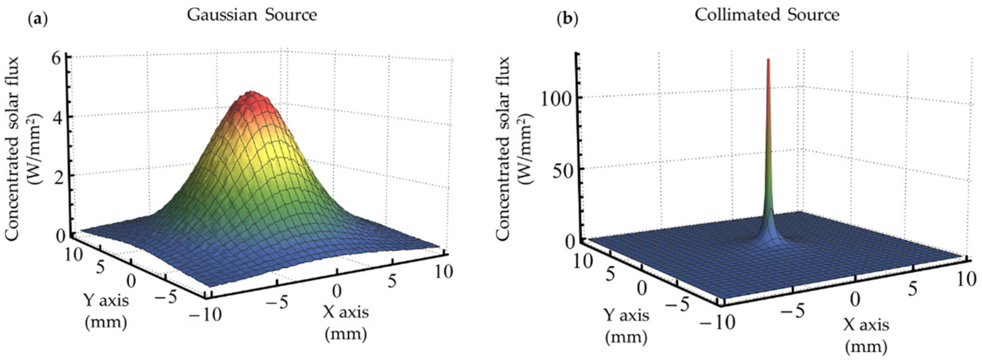
2.2.2. Solar Source Modeling

An “ellipse source” with the same size of the concentrator was used to simulate the solar rays. The total power attributed is given by the product of the concentrator’s collection area and the irradiance, i.e., a 1 m diameter concentrator would have a source power of about 785 W at 1000 W/m² irradiance. Figure 8 shows both the global and the direct reference spectra ASTM (American Society for Testing and Materials) G173 at Air Mass 1.5 (AM1.5) [37]. In Zemax, 21 wavelengths were selected as the solar spectrum data, each normalized as a function of its weight. The weight determines the intensity/power of each solar ray, which is dependent on the power attributed to the emitting source.

The Gaussian distribution of the solar source was defined by Zemax through the G_x and G_y parameters, i.e., the Gaussian distribution parameters in X and Y axes, respectively. These parameters are based on the solar irradiance measured by Vittitoe and Biggs [35].

The root-mean-square width (δ_RMS) adopted by Vittitoe and Biggs, as shown in Equation (17), describes the Sun shape as a function of the irradiance (I).

$${\delta }_{RMS}\times {10}^3\approx 3.7648-0.0038413\left(I-1000\right)+1.5923\times {10}^{-5}{\left(I-1000\right)}^2,$$

(17)

Equation (18) represents the Gaussian distribution of the solar rays from the object “elliptical source” in Zemax. At 1000 W/m² solar irradiance, the Gaussian source would have a value of 35,276.6 at both G_x and G_y axes.

$$G_x=G_y=\frac{1}{2\times {\delta }_{RMS}^2},$$

(18)

Alternatively, the Gaussian distribution of G_x and G_y can be manually adjusted in Zemax based on experimental measurements. For example, in a numerical study of a three-dimensional ring-array concentrator [28], where its output performance was compared to that of the medium sized solar furnace (MSSF) concentrator of PROMES-CNRS (Procédés Matériaux et Energie Solaire—Centre National de la Recherche Scientifique) [38], G_x = G_y = 36,000 was considered [28]. In this case, the solar distribution at the focal zone of the MSSF concentrator had the same characteristics as those described by [38,39,40].

The terrestrial solar half-angle (θ_E) can be calculated by determining the effective size of the solar–terrestrial image (d_E) at a distance (L), as represented in Equation (19).

$${\theta }_E={\tan }^{-1}\left(\frac{0.5 d_E}{L}\right),$$

(19)

θ_E can also be found in Zemax by using a detector at a certain distance from a small solar light source, as shown in Figure 9a. The length L is set as 10 m from the source of 0.002 mm diameter, and the size of the detector (d) as 150 × 150 mm² with a precision of 1001 × 1001 pixels. The calculation of θ_E is independent of the distance L since d_E is adjusted by the inverse-square law.

Figure 9b shows the solar distribution of the solar source obtained from both Equations (17) and (18), considering an irradiance of 1000 W/m² with G_x = G_y = 35,276. For an accurate calculation of the terrestrial solar angle, 95% of the total d_E distribution was considered and θ_E = 0.52° was calculated. It is important to note that the acceptance half-angle (θ_a) of 0.27° can be found at the effective size (d_a) by considering 56% of the focal Gaussian distribution.

2.2.3. Output Solar Distribution at the Focal Zone of the ESFL

To analyze the solar distribution at the focal zone of each ESFL configuration, over 60 million rays were employed per simulation. The output data were obtained from an absorbing detector with dimensions 20 × 20 mm² and resolution 150 × 150 pixels, positioned at the mathematical origin. The obtained data contained the solar distribution characteristics in terms of concentrated solar flux, optical efficiency (the total number of rays that strike the detector over the total emitted rays from the source) and FWHM.

Figure 10 shows the comparison of the three-dimensional focal distributions from a Gaussian source with G_x = G_y = 35,276 and a collimated source with G_x = G_y = 0 (or infinite). In this case, an arbitrary ESFL model with 1 m diameter (D), h_f = 400 mm, h_l = 400 mm, d_t = 3 mm, and δω = 0.20° (256 grooves), with θ_p = 12°, was used. The focal shape formed by the Gaussian source (Figure 9a) has a wide normal distribution with 10.8 mm FWHM and a concentrated solar flux of 5.0 W/mm², while the collimated source (Figure 9b) has a needle-shaped distribution with 0.3 mm FWHM, resulting in a peak concentrated solar flux of more than 100 W/mm². The collimated source offers the highest concentration intensity and its FWHM is nearly as tight as a laser beam. However, this is not possible to obtain with incoherent light provided from the Sun.

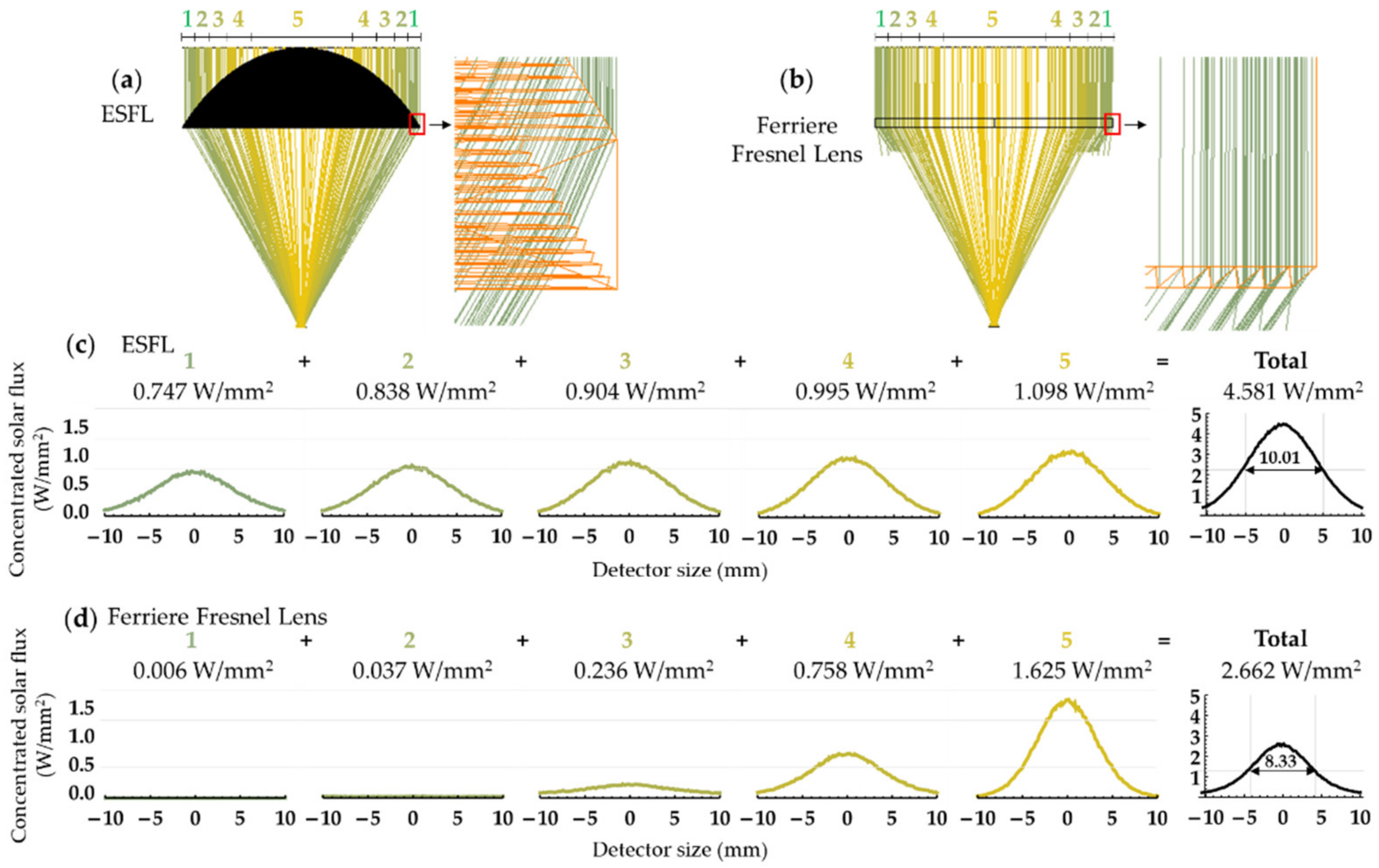
2.2.4. Comparative Study of the ESFL Output Performance with the Measured Output Performance of a Fresnel Lens

Figure 11 shows the simulated layout and the focal output of the ESFL and a flat Fresnel lens [36] at the same focusing conditions. Ferriere et al. used a flat Fresnel lens of 900 mm diameter with 757 mm focal length, 20 grooves/cm (1800 grooves), and 31.7 mm thickness [36]. The measurement was conducted in PROMES-CNRS, where the irradiance can reach 1000 W/m² [36,38,41]. The remaining Fresnel lens parameters were adjusted to achieve the same output performance of the publication, by assuming a conic constant of −1.95 and a modest pitch angle of 2°. By using the solar source Gaussian distribution from [35], the simulated focal output of the flat Fresnel lens in Zemax matched well with the measured data [36]. An ESFL with same collection size and focal length, and h_l = 300 mm, δω = 0.0017° (1807 grooves), d_t = 3 mm and θ_p = 12°, was numerically simulated and compared. Figure 11a,b present the cross-sectional view of the light rays from five concentric annulus solar sources (with same area and power) passing through the ESFL and the Ferriere Fresnel lens, respectively. Area 1 represents the solar rays from the outmost concentric annulus source, while Area 5 corresponds to the solar rays of the innermost circular source. Figure 11c,d show the contribution of each source on the concentrated solar flux of the ESFL and Ferriere Fresnel lens, respectively, as well as the combined concentrated solar fluxes distribution. As shown in Figure 11b, it is noticeable that the solar rays at the external annulus area of the flat Fresnel lens (Area 1 and 2) are barely detected, leading to solar fluxes close to zero (Figure 11d). The curved shaped of the ESFL overcomes this problem, allowing the solar rays from the external annulus area to be more efficiently focused, as demonstrated in Figure 11a,c. Since the external annulus areas collect a majority of the incoming solar power, the advantage of the ESFL concentrator in attaining higher solar flux becomes evident. Chromatic aberration is also significantly reduced, leading finally to a higher concentrated solar flux of 4.5 W/mm² (Figure 11c) compared to that of the flat Fresnel lens with 2.6 W/mm² (Figure 11d) [36]. In addition to the elliptical shape of the Fresnel lens, there are also important factors that can contribute to the better performance of this concentrator, such as the aspect ratio and the number/size of grooves. The influence of these factors on the ESFL output performance is addressed in Section 3.

2.2.5. Comparative Study of the ESFL Output Performance with Other Concentrators

Table 1 shows a summary of some predominant and documented analytical and measured data of other types of concentrators. It is important to note that the experimental data from the existing concentrators should be used as reference in the design and simulation of other concentrators, in order to obtain an accurate and fair evaluation of their performances.

The parabolic mirror of the MSSF had a measured peak concentration of 16 W/mm² with 2000 mm diameter, 850 mm focal length and a focal size of 10 mm FWHM [39]. This parabolic concentrator has currently the highest known concentrated solar flux. However, based on analytical predictions, some authors have claimed higher concentrations with focal width similar to that presented in Figure 10b [12,18,32,42], which is not possible with the incoherent solar light. The focal distribution measurements of linear-shaped Fresnel lenses by O’Neill and McDanal [6] and Leutz et al. [43] had both resulted in much lower concentration solar fluxes of 0.065 W/mm² and 0.045 W/mm², respectively, with the corresponding focal widths of 30 mm and 20 mm. It is common to find much lower concentrations from linear Fresnel lenses. The measured output performance of the flat Fresnel lens presented by Ferriere et al. had a concentrated solar flux of 2.6 W/mm² and a focal size of 8.3 mm at FWHM with a solar irradiance of 1000 W/m² [36]. The present ESFL, at the same conditions of the flat Fresnel lens from [36], had a better focal solar flux of 4.5 W/mm².

Table 1. Focal concentration and size from various concentrator types found in some publications.

Publications	Concentrator Type	Concentration	Focal Width (mm)	Lens Width (mm)	Focal Length(mm)	Grooves Per mm	Method
Nelson et al., 1975 [44]	Fresnel lens	4.3–5.0 (ratio)	~30	137	140	~0.1	Analytical
Cosby, 1977 [5]	Shaped Fresnel lens (linear)	~70 (ratio)	~20	~914	~509	~1.0	Analytical
Kritchman et al., 1979 [7]	Shaped Fresnel lens (linear)	172 (ratio)	N/A	vary	vary	Infinitely small grooves	Analytical
O’Neill et al., 1993 [6]	Shaped Fresnel lens (linear)	0.065 (W/mm2)	~30	850	726	N/A	Experimental
Flamant et al., 1999 [39]	Parabolic mirror	16.0 (W/mm2)	~16 ~10 (FWHM)	2000	850	N/A	Experimental
Leutz et al., 2000 [43]	Shaped Fresnel lens (linear)	0.045 (W/mm2)	~20 ~5–6 (FWHM)	~300	~150	N/A	Experimental
Ferriere et al., 2004 [36]	Flat Fresnel lens	2.644 (W/mm2)	~20 ~8.3 (FWHM)	900	757	2.0	Experimental
Yeh, 2009, [24]	Shaped Fresnel lens (linear)	0.060 (W/mm2)	~5–6 (FWHM)	300	446	1.0	Analytical
Pan et al., 2011 [32]	Fresnel lens	1,367,704,600 (W/mm2)	<0.25	189	189	N/A	Analytical
Akisawa et al., 2012 [10]	Shaped Fresnel lens	0.506 (W/mm2)	<1	45	60	4.0	Analytical
Cheng et al., 2013b [18]	Fresnel lens	N/A	<0.1	88	50	0.22	Analytical
Languy et al., 2013 [12]	Shaped Fresnel lens	8500 (ratio)	<1	N/A	N/A	N/A	Analytical
Yeh, 2016 [21]	Shaped Fresnel lens (linear)	0.070 (W/mm2) (at 1135 nm)	~20 ~4 (FWHM)	300	223	2.0	Analytical
Yeh et al., 2016 [22]	Shaped Fresnel lens	~5.0 (W/mm2)	~20 ~4 (FWHM)	460	280	4.3	Analytical
Zhao et al., 2018 [33]	Shaped Fresnel lens (linear)	40.6 (ratio)	16	650	950	N/A	Experimental
Garcia et al., 2019 [28]	RAC 1	16.0 (W/mm2)	~20 ~10 (FWHM)	2000	500	N/A	Analytical
Liang et al., 2021 [42]	AFSCFL 2	46.7 (W/mm2)	<1	734	593	N/A	Analytical
Present work	Shaped Fresnel lens	4.5 (W/mm2)	~10.0 (FWHM)	900	757	0.34	Analytical

¹ Ring array concentrator. ² Annular Fresnel solar concentrator coupled with a circular Fresnel lens.

Table 1. Focal concentration and size from various concentrator types found in some publications.

Publications	Concentrator Type	Concentration	Focal Width (mm)	Lens Width (mm)	Focal Length(mm)	Grooves Per mm	Method
Nelson et al., 1975 [44]	Fresnel lens	4.3–5.0 (ratio)	~30	137	140	~0.1	Analytical
Cosby, 1977 [5]	Shaped Fresnel lens (linear)	~70 (ratio)	~20	~914	~509	~1.0	Analytical
Kritchman et al., 1979 [7]	Shaped Fresnel lens (linear)	172 (ratio)	N/A	vary	vary	Infinitely small grooves	Analytical
O’Neill et al., 1993 [6]	Shaped Fresnel lens (linear)	0.065 (W/mm2)	~30	850	726	N/A	Experimental
Flamant et al., 1999 [39]	Parabolic mirror	16.0 (W/mm2)	~16 ~10 (FWHM)	2000	850	N/A	Experimental
Leutz et al., 2000 [43]	Shaped Fresnel lens (linear)	0.045 (W/mm2)	~20 ~5–6 (FWHM)	~300	~150	N/A	Experimental
Ferriere et al., 2004 [36]	Flat Fresnel lens	2.644 (W/mm2)	~20 ~8.3 (FWHM)	900	757	2.0	Experimental
Yeh, 2009, [24]	Shaped Fresnel lens (linear)	0.060 (W/mm2)	~5–6 (FWHM)	300	446	1.0	Analytical
Pan et al., 2011 [32]	Fresnel lens	1,367,704,600 (W/mm2)	<0.25	189	189	N/A	Analytical
Akisawa et al., 2012 [10]	Shaped Fresnel lens	0.506 (W/mm2)	<1	45	60	4.0	Analytical
Cheng et al., 2013b [18]	Fresnel lens	N/A	<0.1	88	50	0.22	Analytical
Languy et al., 2013 [12]	Shaped Fresnel lens	8500 (ratio)	<1	N/A	N/A	N/A	Analytical
Yeh, 2016 [21]	Shaped Fresnel lens (linear)	0.070 (W/mm2) (at 1135 nm)	~20 ~4 (FWHM)	300	223	2.0	Analytical
Yeh et al., 2016 [22]	Shaped Fresnel lens	~5.0 (W/mm2)	~20 ~4 (FWHM)	460	280	4.3	Analytical
Zhao et al., 2018 [33]	Shaped Fresnel lens (linear)	40.6 (ratio)	16	650	950	N/A	Experimental
Garcia et al., 2019 [28]	RAC 1	16.0 (W/mm2)	~20 ~10 (FWHM)	2000	500	N/A	Analytical
Liang et al., 2021 [42]	AFSCFL 2	46.7 (W/mm2)	<1	734	593	N/A	Analytical
Present work	Shaped Fresnel lens	4.5 (W/mm2)	~10.0 (FWHM)	900	757	0.34	Analytical

¹ Ring array concentrator. ² Annular Fresnel solar concentrator coupled with a circular Fresnel lens.

3. Output Performance of the ESFL Regarding the Concentrated Solar Flux, the Optical Efficiency and the FWHM

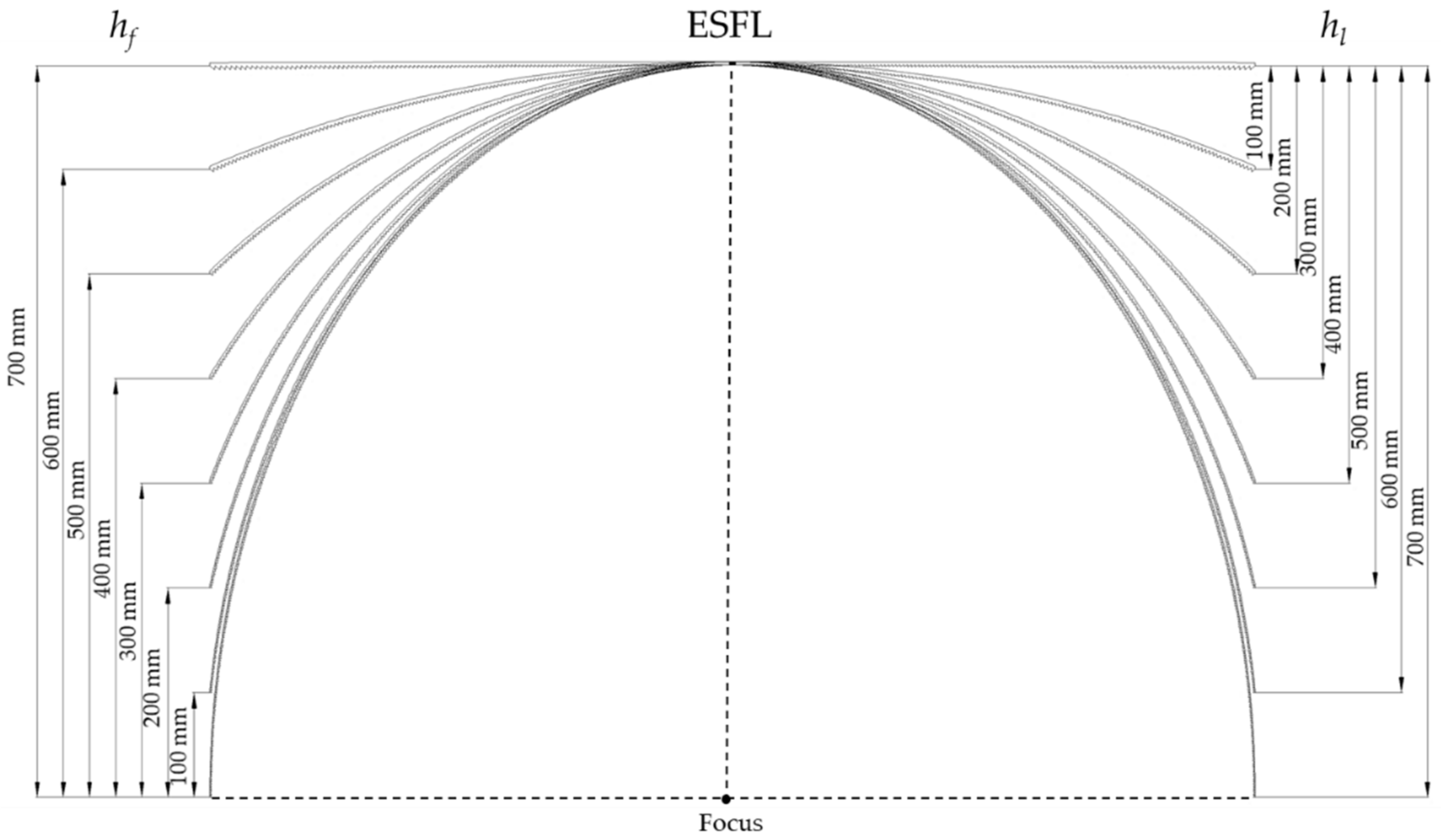
3.1. ESFL Configurations with Fixed Total Height of 700 mm

As any lens, the shape of the ESFL concentrator has direct influence on its output performance. Figure 12 shows some of the possible configurations of the ESFL with a combined h_f and h_l of 700 mm total height.

The ESFL has a similar configuration of a flat Fresnel lens at h_f = 700 mm, h_l = 0 mm. As h_l increases, the lens becomes more curved, and the aspect ratio becomes larger. The aspect ratio (AR) of the ESFL is given by the quotient of h_l and D (diameter of the lens):

$$AR=\frac{h_l}{D},$$

(20)

Figure 13 shows the variation of the concentrated solar flux as a function of the aspect ratio of ESFL and h_l, with 700 mm total height. All the ESFL configurations had D = 1 m, δ_ω = 0.28°, θ_p = 12° and d_t = 3 mm. The concentrated solar flux starts with 3.9 W/m² at h_l = 0 mm, which closely resembles that of a flat Fresnel lens. It gradually increases with h_l, at which point the Fresnel lens is shaped into a parabola. The concentrated solar flux is maintained over 5.2 W/mm² from h_l of 500 mm to 700 mm, i.e., with aspect ratio from 0.603 to 0.702.

3.2. Concentrated Solar Flux, Optical Efficiency and FWHM as a Function of the Aspect Ratio and Several Combinations of h_f + h_l

Figure 14 shows the concentrated solar flux, optical efficiency and FWHM at various combinations of h_f and h_l with ESFLs of D = 1 m, δ_ω = 0.28°, θ_p = 12° and d_t = 3 mm. h_f ranges from 200 mm to 600 mm and h_l ranges from 50 mm to at least 500 mm.

Each h_f has its own peak concentrated solar flux at different h_l (Figure 14a). For example, in the ESFL configuration with h_f = 200 mm, the concentrated solar flux varies from 4.2 W/mm² at h_l = 50 mm to 5.2 W/mm² at h_l = 500 mm, above which it starts to decrease. The highest concentrated solar flux was attained by the lowest h_f = 200 mm at h_l = 500 mm (aspect ratio of 0.603). The increase in h_f resulted in a lower concentrated solar flux, whose peak value shifted to a lower h_l, decreasing the aspect ratio of the concentrator. For example, the ESFL with h_f = 600 mm has an aspect ratio of 0.500 with h_l = 350 mm and a concentrated solar flux of 4.4 W/mm².

The optical efficiency tends to stagnate at larger h_l, as shown in Figure 14b. The highest optical efficiency of about 60% was attained at the higher h_f of 600 mm. The FWHM enlarges in a near linear fashion with the increase in h_l, and it also expands with the increase in h_f, as shown in Figure 14c.

3.3. Influence of Size/Number of Grooves on the ESFL Output Performance

The influence of different sizes of δω on the ESFL output performance was analyzed for the most favorable combinations of h_f and h_l that achieved the highest concentrated solar fluxes (Figure 14a). The variation of δω changes the size of each groove/prism within the ESFL concentrator, mainly changing the size of the input (A_nB_n) and the output (A_nD_n) facets, as calculated in Equations (9) and (15). A range of δω, from 0.05° to 1°, was used for the conception of the ESFL model. Figure 15a shows the number of grooves per δω at different h_f. The number of grooves drops exponentially independently of the h_f with the increase in δω. A gap in the number of grooves between h_f is observed at a smaller δω, while it converges closer into the same number of grooves at a larger δω.

Figure 15b shows the concentrated solar flux as a function of δω. Regardless of h_f, the maximum concentrated solar flux was found at δω = 0.3°, which is equivalent to 210 to 132 grooves for h_f 200 mm to 600 mm, respectively. As shown in Figure 15c, the increase in δω lowers the optical efficiency from 66% to 56% and 53% to 50% at h_f of 600 mm and 200 mm, respectively. The FWHM shows a minimum within a certain δω range, as shown in Figure 15d. For example, at h_f = 600 mm, more than 10.7 mm FWHM was found at δω = 0.35°, while at h_f = 200 mm, the minimum FWHM of about 8 mm was found at δω = 0.2°. In all cases, the largest FWHM is located at δω = 1°.

The number of grooves has a direct influence on the focal characteristics of the concentrator, as demonstrated in Figure 16. On the one hand, with the increasing number of grooves (lower δω), each prism becomes smaller, which reduces the refraction space within the prism. Consequently, above a certain number of grooves, the number of effective rays that could be refracted onto the targeted focal position is diminished, causing the decrease in the concentrated solar flux, as illustrated in Figure 16b. On the other hand, the reduction in the number of grooves (higher δω) leads to an increment in the size of the prism, hence broadening the final output focal shape, as shown in Figure 16d. Therefore, the concentration solar flux also diminishes with the decrease in the number of grooves (Figure 16b). Maximum concentrated solar flux was numerically found at δω = 0.30° for all the ESFLs, regardless the h_f, as demonstrated in both Figure 15b and Figure 16b. However, the optimum number of grooves varies with h_f. Consequently, for δω = 0.30°, the optimum number of grooves varied from 227 grooves with h_f = 200 mm to 132 grooves with h_f = 600 mm, corresponding to 0.42 grooves/mm and 0.26 grooves/mm, respectively. This variation is even more pronounced with smaller δω (higher number of grooves). The optimum groove number per size is by far lower than that of other Fresnel lenses (Table 1), such as the shaped Fresnel lens with 4.3 groove/mm at D = 460 mm [22], flat Fresnel lens with 2 grooves/mm at D = 900 mm [36], 2 grooves/mm at D = 889 mm [45], and a range of 15.7 grooves/mm to 1 grooves/mm at various sizes of Fresnel lenses found at the market, such as the Fresneltech [25]. The higher performance of the ESFL with larger prisms and, consequently, lower number of grooves is attributed to the fact that the design process was not under the influence of the common modeling processes based on the edge-ray principle, but based on the solar Gaussian distribution. The reduction in the number of grooves and subsequent increase in the prism size could be favorable for the manufacturer in neglecting the limit losses due to manufacturing inaccuracies, such as blunt tips and deformed grooves forming.

4. Comparison between ESFL and a Flat Fresnel Lens

4.1. Optimal Focal Position Analysis of Both the ESFL and a Flat Fresnel Lens

Figure 17 and Figure 18 show the three-dimensional light distribution along the focal zone of the ESFL and a flat Fresnel lens with the same collection size, respectively. The ESFL had D = 1 m, δ_ω = 0.28° (171 grooves), θ_p = 12°, d_t = 3 mm, h_f = 300 mm, and h_l = 450 mm. The flat Fresnel lens with the highest concentration flux configuration was chosen, with D = 1 m, h_f = 400 mm, 0.3 grooves per mm (150 grooves) and θ_p = 12°. The focal cones, as shown in Figure 17a and Figure 18a, were represented by a detector volume with 100 × 100 × 100 voxels in vacuum, where each voxel accumulates and stores the energy data from each ray that passes through it, with the associated wavelength and power. Figure 17b shows the top view focal distribution of the ESFL in the detector positioned at the origin (Z = 0 mm), with a concentrated solar flux of 5.08 W/mm², while Figure 17c shows the focal distribution at Z = −5 mm in relation to the origin, with a maximum concentrated solar flux of 5.48 W/mm². Figure 18b shows the focal distribution of the flat Fresnel lens at Z = 0 mm, with a concentrated solar flux of 0.75 W/mm². At Z = +30 mm in relation to the origin, the maximum concentrated solar flux of only 1.86 W/mm² was reached, as shown in Figure 18c.

For both the ESFL and the flat Fresnel lens, the focal distributions at the origin (Z = 0 mm) do not correspond to the positions where the concentrated solar flux is maximum, as shown in Figure 17a and Figure 18a. This phenomenon occurs due to the chromatic aberration, which is more abundant in the flat Fresnel lens. It is important to note that a parabolic concentrator (a concentrator with no chromatic aberration effect) has its maximum concentration exactly at the origin point [28].

4.2. Temperature Analysis of Both the ESFL and the Flat Fresnel Lens

Zemax non-sequential ray-tracing and Ansys finite element analyses were both used to evaluate the temperature of both the ESFL and the flat Fresnel lens at the Z position with the highest concentration solar flux found in Section 4.1. Ansys allows thermo-optical calculations that deal with complex geometric shape and boundary conditions, enabling the approximation of variables in a volume or surface element that changes across the matrix [46,47,48].

In Zemax, a square absorbing black body (emissivity ε = 1 [49]) detector of 20 × 20 mm² and 150 × 150 pixels was used to calculate the concentrated solar flux at the optimal focal positions of the ESFL and the flat Fresnel lens. The matrixial data were then exported to the Ansys workbench through the “External data” component and loaded as a heat flux source.

In Ansys 2021 finite element analysis, a graphite disk receiver of 20 mm diameter and 5 mm thickness was used to obtain the temperature of both concentrators. The graphite of 2250 kg/m³ constant density, 24 W/m K thermal conductivity and 709 J/Kg K specific heat were chosen from the Ansys internal material library. The disk receiver was divided by the tetrahedrons meshing method with a sizing element of 0.4 mm. It contained approximately 1600 elements, which were enough for FEA calculations, with good approximation. The boundary conditions set for the convection applied onto the disk were the same as the natural stagnant air convection, representing a heat transfer coefficient of 5 × 10⁻⁶ W/mm²/K. The radiation exchange between surfaces was restricted by a gray-diffused surface and the emissivity for the graphite disk surface was confined to ε = 0.85. A room temperature of 295.15 K was considered.

The respective temperatures of the ESFL and the flat Fresnel lens are shown in Figure 19. Both temperatures were generated from the focal distributions of Figure 17c and Figure 18b, respectively. The ESFL attained maximum and minimum temperatures of 2362 K and 1945 K, respectively, which were 1.73 and 1.60 times more than that of the Fresnel lens with the maximum temperature of 1363 K and minimum temperature of 1217 K, respectively.

5. Conclusions

To overcome the aberration chromatic issue of Fresnel lens concentrators, a novel parametric model of a three-dimensional elliptical-shaped Fresnel lens was provided and analyzed. The modeling process took into account the solar Gaussian distribution based on the measured parameters by Vittitoe and Biggs [35], instead of the classical edge-ray principle method and the solar acceptance half-angle of 0.27°. The design was performed by CAD software and then imported into Zemax for numerical calculations. The accuracy of this model was confirmed by the numerical analysis of the output performance of a flat Fresnel, whose results matched well with the experimental data [36]. The ESFL output performance was compared to these results, under the same focusing conditions, revealing the advantage of the ESFL in focusing more efficiently the solar rays from the external annulus area, at the external annulus collection area, where a significant part of the incoming solar power is collected, resulting in a significant increase in the concentrated solar flux.

The study of different combinations of ESFL focal length and arch height, and their influence on the output performance was carried out. The highest peak solar flux of about 5.2 W/m² was attained for the ESFL with a shorter focal length of h_f = 200 mm and high arch height of h_l = 500 mm, resulting in a large aspect ratio of 0.603. As h_f increased, the solar concentration decreased, but maximum solar fluxes were attained with a smaller h_l, hence lowering the aspect ratio.

The optimal concentrated solar flux value within the focal cone of the best ESFL was then studied and compared to that of a flat Fresnel lens at its best output performance configuration. This study demonstrated the effectiveness of the ESFL in reducing the chromatic aberration, leading to a significant enhancement of the concentrated solar flux and temperature, as compared to that of the flat Fresnel lens.

In addition, the present work also provided a comprehensive study of the influence of the number of grooves and size on the ESFL performance. It was found that the optimal number of groves per millimeter could be substantially reduced in relation to that reported by the previous literature and market. This could greatly facilitate the manufacturing process of Fresnel lens concentrators while increasing its solar concentration capacity, revealing the promising potential of ESFL in many solar energy research and applications.

References

1. Price, J.S.; Sheng, X.; Meulblok, B.M.; Rogers, J.A.; Giebink, N.C. Wide-angle planar microtracking for quasi-static microcell concentrating photovoltaics. Nat. Commun. 2015, 6, 6223. [Google Scholar] [CrossRef] [PubMed]
2. Coughenour, B.M.; Stalcup, T.; Wheelwright, B.; Geary, A.; Hammer, K.; Angel, R. Dish-based high concentration PV system with Köhler optics. Opt. Express 2014, 22, A211–A224. [Google Scholar] [CrossRef] [PubMed]
3. El Majid, B.; Motahhir, S.; El Ghzizal, A. Parabolic bifacial solar panel with the cooling system: Concept and challenges. SN Appl. Sci. 2019, 1, 1176. [Google Scholar] [CrossRef] [Green Version]
4. Xie, W.T.; Dai, Y.J.; Wang, R.Z.; Sumathy, K. Concentrated solar energy applications using Fresnel lenses: A review. Renew. Sustain. Energy Rev. 2011, 15, 2588–2606. [Google Scholar] [CrossRef]
5. Cosby, R.M. Solar Concentration by Curved-Base Fresnel Lenses; Ball State University: Muncie, IN, USA, 1977. [Google Scholar]
6. Neill, M.J.O.; McDanal, A.J. Manufacturing Technology Improvements for a Line-Focus Concentrator Module. In Proceedings of the Twenty Third IEEE Photovoltaic Specialists Conference—1993, Conference Record (Cat. No.93CH3283-9). Louisville, KY, USA, 10–14 May 1993; pp. 1082–1089. [Google Scholar]
7. Kritchman, E.M.; Friesem, A.A.; Yekutieli, G. Highly Concentrating Fresnel Lenses. Appl. Opt. 1979, 18, 2688–2695. [Google Scholar] [CrossRef]
8. Leutz, R.; Suzuki, A.; Akisawa, A.; Kashiwagi, T. Design of a nonimaging Fresnel lens for solar concentrators. Sol. Energy 1999, 65, 379–387. [Google Scholar] [CrossRef]
9. Yeh, N. Analysis of spectrum distribution and optical losses under Fresnel lenses. Renew. Sustain. Energy Rev. 2010, 14, 2926–2935. [Google Scholar] [CrossRef]
10. Akisawa, A.; Hiramatsu, M.; Ozaki, K. Design of dome-shaped non-imaging Fresnel lenses taking chromatic aberration into account. Sol. Energy 2012, 86, 877–885. [Google Scholar] [CrossRef]
11. Romero, M.; Steinfeld, A. Concentrating solar thermal power and thermochemical fuels. Energy Environ. Sci. 2012, 5, 9234–9245. [Google Scholar] [CrossRef]
12. Languy, F.; Habraken, S. Nonimaging achromatic shaped Fresnel lenses for ultrahigh solar concentration. Opt. Lett. 2013, 38, 1730–1732. [Google Scholar] [CrossRef]
13. Ma, X.; Zheng, H.; Tian, M. Optimize the shape of curved-Fresnel lens to maximize its transmittance. Sol. Energy 2016, 127, 285–293. [Google Scholar] [CrossRef]
14. Leutz, R.; Suzuki, A. Nonimaging Fresnel Lenses: Design and Performance of Solar Concentrators; Springer Science & Business Media: Berlin/Heidelberg, Germany, 2001. [Google Scholar]
15. Kalogirou, S. Solar Energy Engineering Processes and Systems; Academic Press: Cambridge, MA, USA, 2013. [Google Scholar]
16. Rabl, A. Active Solar Collectors and Their Applications; Oxford University Press on Demand: Oxford, UK, 1985. [Google Scholar]
17. Winston, R. Principles of Solar Concentrators of a Novel Design. Sol. Energy 1974, 16, 89–95. [Google Scholar] [CrossRef]
18. Cheng, Y.; Zhang, X.D.; Zhang, G.X. Design and machining of Fresnel solar concentrator surfaces. Int. J. Precis. Technol. 2013, 3, 354–369. [Google Scholar] [CrossRef]
19. Zheng, H.; Feng, C.; Su, Y.; Dai, J.; Ma, X. Design and experimental analysis of a cylindrical compound Fresnel solar concentrator. Sol. Energy 2014, 107, 26–37. [Google Scholar] [CrossRef]
20. Viera-González, P.M.; Sánchez-Guerrero, G.E.; Martínez-Guerra, E.; Ceballos-Herrera, D.E. Mathematical Analysis of Nonimaging Fresnel Lenses Using Refractive and Total Internal Reflection Prisms for Sunlight Concentration. Math. Probl. Eng. 2018, 2018, 4654795. [Google Scholar] [CrossRef]
21. Yeh, N. Illumination uniformity issue explored via two-stage solar concentrator system based on Fresnel lens and compound flat concentrator. Energy 2016, 95, 542–549. [Google Scholar] [CrossRef]
22. Yeh, N.; Yeh, P. Analysis of point-focused, non-imaging Fresnel lenses’ concentration profile and manufacture parameters. Renew. Energy 2016, 85, 514–523. [Google Scholar] [CrossRef]
23. Ma, X.; Jin, R.; Liang, S.; Zheng, H. Ideal shape of Fresnel lens for visible solar light concentration. Opt. Express 2020, 28, 18141–18149. [Google Scholar] [CrossRef]
24. Yeh, N. Optical geometry approach for elliptical Fresnel lens design and chromatic aberration. Sol. Energy Mater. Sol. Cells 2009, 93, 1309–1317. [Google Scholar] [CrossRef]
25. Fresneltech Brochure. Available online: https://www.fresneltech.com/fresnel-lenses (accessed on 17 June 2021).
26. Garcia-Segura, A.; Fernandez-Garcia, A.; Ariza, M.J.; Sutter, F.; Valenzuela, L. Durability studies of solar reflectors: A review. Renew. Sustain. Energy Rev. 2016, 62, 453–467. [Google Scholar] [CrossRef] [Green Version]
27. He, C.; Duan, X.; Zhao, Y.; Feng, J. An analytical flux density distribution model with a closed-form expression for a flat heliostat. Appl. Energy 2019, 251, 113310. [Google Scholar] [CrossRef]
28. Garcia, D.; Liang, D.; Tibúrcio, B.D.; Almeida, J.; Vistas, C.R. A three-dimensional ring-array concentrator solar furnace. Sol. Energy 2019, 193, 915–928. [Google Scholar] [CrossRef]
29. Lv, H.; Huang, X.; Li, J.; Huang, W.; Li, Y.; Su, Y. Non-uniform sizing of PV cells in the dense-array module to match the non-uniform illumination in dish-type CPV systems. Int. J. Low-Carbon Technol. 2020, 15, 565–573. [Google Scholar] [CrossRef]
30. Garcia, D.; Liang, D.; Almeida, J.; Tibúrcio, B.D.; Costa, H.; Catela, M.; Vistas, C.R. Analytical and numerical analysis of a ring-array concentrator. Int. J. Energy Res. 2021, 45, 15110–15123. [Google Scholar] [CrossRef]
31. Yeh, P.; Yeh, N. Design and analysis of solar-tracking 2D Fresnel lens-based two staged, spectrum-splitting solar concentrators. Renew. Energy 2018, 120, 1–13. [Google Scholar] [CrossRef]
32. Pan, J.-W.; Huang, J.-Y.; Wang, C.-M.; Hong, H.-F.; Liang, Y.-P. High concentration and homogenized Fresnel lens without secondary optics element. Opt. Commun. 2011, 284, 4283–4288. [Google Scholar] [CrossRef]
33. Zhao, Y.; Zheng, H.; Sun, B.; Li, C.; Wu, Y. Development and performance studies of a novel portable solar cooker using a curved Fresnel lens concentrator. Sol. Energy 2018, 174, 263–272. [Google Scholar] [CrossRef]
34. Shen, F.; Huang, W. Study on the Optical Properties of the Point-Focus Fresnel System. Sustainability 2021, 13, 10367. [Google Scholar] [CrossRef]
35. Vittitoe, C.N.; Biggs, F. Six-gaussian representation of the angular-brightness distribution for solar radiation. Sol. Energy 1981, 27, 469–490. [Google Scholar] [CrossRef]
36. Ferriere, A.; Rogriguez, G.; Sobrino, J. Flux Distribution Delivered by a Fresnel Lens Used for Concentrating Solar Energy. J. Sol. Energy Eng. 2004, 126, 654–660. [Google Scholar] [CrossRef]
37. ASTM International Standard Tables for Reference Solar Spectral Irradiance at Air Mass 1.5: Direct Normal and Hemispherical for a 37 Degree Tilted Surface. Available online: https://www.nrel.gov/grid/solar-resource/spectra-am1.5.html (accessed on 21 December 2021).
38. MEÉSU Procédés. MSSF horizontal—PROMES. Available online: https://www.promes.cnrs.fr/index.php?page=mssf-horizontal (accessed on 7 March 2019).
39. Flamant, G.; Ferriere, A.; Laplaze, D.; Monty, C. Solar Processing of Materials: Opportunities and New Frontiers. Sol. Energy 1999, 66, 117–132. [Google Scholar] [CrossRef]
40. Ferriere, A.; Sanchez Bautista, C.; Rodriguez, G.P.; Vazquez, A.J. Corrosion resistance of stainless steel coatings elaborated by solar cladding process. Sol. Energy 2006, 80, 1338–1343. [Google Scholar] [CrossRef]
41. Gineste, J.M.; Flamant, G.; Olalde, G. Incident solar radiation data at Odeillo solar furnaces. J. Phys. IV 1999, 9, Pr3-623–Pr3-628. [Google Scholar] [CrossRef]
42. Liang, K.; Zhang, H.; Chen, H.; Gao, D.; Liu, Y. Design and test of an annular fresnel solar concentrator to obtain a high-concentration solar energy flux. Energy 2021, 214, 118947. [Google Scholar] [CrossRef]
43. Leutz, R.; Suzuki, A.; Akisawa, A.; Kashiwagi, T. Shaped nonimaging Fresnel lenses. J. Opt. A Pure Appl. Opt. 2000, 2, 112–116. [Google Scholar] [CrossRef]
44. Nelson, D.T.; Evans, D.L.; Bansal, R.K. Linear Fresnel Lens Concentrators. Sol. Energy 1975, 17, 285–289. [Google Scholar] [CrossRef]
45. Sierra, C.; Vázquez, A. NiAl coatings on carbon steel by self-propagating high-temperature synthesis assisted with concentrated solar energy: Mass influence on adherence and porosity. Sol. Energy Mater. Sol. Cells 2005, 86, 33–42. [Google Scholar] [CrossRef]
46. An, W.; Ruan, L.M.; Qi, H.; Liu, L.H. Finite element method for radiative heat transfer in absorbing and anisotropic scattering media. J. Quant. Spectrosc. Radiat. Transf. 2005, 96, 409–422. [Google Scholar] [CrossRef]
47. Li, B.; Oliveira, F.A.C.; Rodriguez, J.; Fernandes, J.C.; Rosa, L.G. Numerical and experimental study on improving temperature uniformity of solar furnaces for materials processing. Sol. Energy 2015, 115, 95–108. [Google Scholar] [CrossRef]
48. Rinker, G.; Solomon, L.; Qiu, S.G. Optimal placement of radiation shields in the displacer of a Stirling engine. Appl. Therm. Eng. 2018, 144, 65–70. [Google Scholar] [CrossRef]
49. Radiant Zemax. Zemax Manual; Radiant Zemax: Sacramento, CA, USA, 2014; Volume 13. [Google Scholar]
Figure 1. (a) Cross-sectional representation of an elliptical-shaped Fresnel lens (ESFL). 2θa represents the subtended angle of the Sun to the Earth and E the solar–terrestrial angle after the passage of the solar rays through the atmosphere. (b) 3D representation of the ESFL.
Energies 15 00668 g001
Figure 2. Segment of an ellipse used as an outline for ESFL. “a” and “b” are the major and minor axis of the ellipse. “b” is the sum of the height of the arch (hl) and the focal length (hf) and ω is the rim angle of the Fresnel lens.
Energies 15 00668 g002
Figure 3. (a) Representation of a half-segment of an ESFL. The region defined by point A to B represents the first segment of the ellipse and the input facet of the first prism. The size of the prism is defined by angle δω. The point O represents the origin point and focal zone. AO and BO are the distances between the focal zone with the vertexes A and B of the prism, respectively. (b) Detailed visualization of a single prism. The incoming solar rays are refracted by the prism, outputting an angle ω in relation to the normal of its output facet, thus guaranteeing the concentration of light to the focal zone. AB segment is the input facet. Both AC and AD segments represent the output facet, whereas both BC and BD represent the back facet. The pitch angle (θp) defines the unused part of the prism.
Energies 15 00668 g003
Figure 4. Chaining process of the first three prisms of the ESFL. The thickness of the concentrator is attributed by offsetting the input facet by dt from its original coordinate position.
Energies 15 00668 g004
Figure 5. Flowchart of ESFL modeling process.
Energies 15 00668 g005
Figure 6. Sequence diagram of a single numerical simulation.
Energies 15 00668 g006
Figure 7. 3D view of the ESFL in AutoCAD.
Energies 15 00668 g007
Figure 8. Global and direct solar spectra ASTMG173 at AM1.5, with the selected wavelength used for ray tracing in Zemax and its respective weight value.
Energies 15 00668 g008
Figure 9. (a) Light propagation from a small light source towards a detector of size d at distance L. (b) Solar–terrestrial image with solar half-angle (θE) of 0.52°.
Energies 15 00668 g009
Figure 10. The focal image formed by ESFL modeled at 1000 W/mm2 irradiance with the (a) Gaussian source and (b) collimated source.
Energies 15 00668 g010
Figure 11. (a) The ESFL and (b) the Ferriere Fresnel lens irradiated by five concentric solar sources with identical area and power. (c,d) Respective concentrated solar fluxes for the ESFL and the Ferriere lens, respectively; the combined solar fluxes are also given.
Energies 15 00668 g011
Figure 12. ESFL configuration with a combination of hf and hd for a total height of 700 mm.
Energies 15 00668 g012
Figure 13. Concentrated solar flux of the ESFL with a combined hf + hd of 700 mm as a function of hl and aspect ratio.
Energies 15 00668 g013
Figure 14. (a) Concentrated solar flux, (b) optical efficiency and (c) FWHM of the ESFL configurations with D = 1 m at various hf and hl combinations.
Energies 15 00668 g014
Figure 15. Characteristics of the Gaussian distribution source at the focal zone: (a) number of grooves per δω, (b) concentrated solar flux, (c) optical efficiency and (d) FWHM.
Energies 15 00668 g015
Figure 16. Characteristic of the Gaussian distribution source at the focal zone: (a) δω, (b) concentrated solar flux, (c) optical efficiency and (d) FWHM as a function of the number of grooves.
Energies 15 00668 g016
Figure 17. (a) Three-dimensional focal distribution of the ESFL. (b) Top view of the light distribution at the focal point (Z = 0 mm). (c) Top view of the light distribution with the highest concentrated solar flux (Z = −5 mm).
Energies 15 00668 g017
Figure 18. (a) Three-dimensional focal distribution of the flat Fresnel lens. (b) Top view of the light distribution at the focal point (Z = 0 mm). (c) Top view of the light distribution with the highest concentrated solar flux (Z = 30 mm).
Energies 15 00668 g018
Figure 19. Focal temperature of ESFL (a) and flat Fresnel lens (b).
Energies 15 00668 g019
Publisher’s Note: MDPI stays neutral with regard to jurisdictional claims in published maps and institutional affiliations.